báo cáo hóa học:" Landscape features and weather influence nest survival of a ground-nesting bird of conservation concern, the greater sage-grouse, in humanaltered environments" ppt

RESEARCH Open Access
Landscape features and weather influence nest
survival of a ground-nesting bird of conservation
concern, the greater sage-grouse, in human-
altered environments
Stephen L Webb
1*
, Chad V Olson
1
, Matthew R Dzialak
1
, Seth M Harju
1
, Jeffrey B Winstead
1
and Dusty Lockman
2
Abstract
Introduction: Ground-nesting birds experience high levels of nest predation. However, birds can make selection
decisions related to nest site location and characteristics that may result in physical, visual, and olfactory
impediments to predators.
Methods: We studied daily survival rate [DSR] of greater sage-grouse (Centrocercus urophasianus) from 2008 to
2010 in an area in Wyoming experiencing large-scale alterations to the landscape. We used generalized linear
mixed models to model fixed and random effects, and a correlation within nesting attempts, individual birds, and
years.
Results: Predation of the nest was the most common source of nest failure (84.7%) followed by direct predation of
the female (13.6%). Generally, landscape variables at the nest site (≤ 30 m) were more influential on DSR of nests
than features at larger spatial scales. Percentage of shrub canopy cover at the nest site (15-m scale) and distances
to natural gas wells and mesic areas had a positive relat ionship with DSR of nests, whereas distance to roads had a
negative relationship with DSR of nests. When added to the vegetation model, maximum wind speed on the day
of nest failure and a 1-day lag in precipitation (i.e., precipitation the day before failure) improved model fit

whereby both variables negatively influenced DSR of nests.
Conclusions: Nest site characteristics that reduce visibility (i.e., shrub canopy cover) have the potential to reduce
depredation, whereas anthropogenic (i.e., distance to wells) and mesic landscape features appear to facilitate
depredation. Last, predators may be more efficient at locating nests under certain weather conditions (i.e., high
winds and moisture).
Keywords: behavior, Centrocercus urophasianus, conservation, depredation, generalized linear mixed models,
greater sage-grouse, human development, management, nest survival, weather
Introduction
Predators can influence and regulate prey populations
(Crooks and Soulé 1999). A primary example of this is
through nest depredation (Gregg et al. 1994; Conway
and Martin 2000; Chalfoun et al. 2002; Holloran et al.
2005; Stephens et al. 2005; Moynahan et al. 2007). Nest
success, often defined as having ≥ 1 egg hatch, is
influenced strongly by the choices females make in
terms of nest placement because local and landscape-
level features of the nest site are correlated with sus-
ceptibility to depredation (Lima 2009; Conover et al.
2010). Often, females select for screening cover at the
nest site to reduce detection by visually oriented preda-
tors. In certain situations, ground-nesting birds can
place nests in favorable settings to reduce both visual
and olfactory detection, but many times, the selection
for concealment from visually oriented predators occurs
at the expense of olfactory detection (Conover and
* Correspondence:
1
Hayden-Wing Associates, LLC, 2308 South 8th Street, Laramie, WY, 82070,
USA
Full list of author information is available at the end of the article

Webb et al. Ecological Processes 2012, 1:1
/>© 2012 Webb et al; licensee Springer. This is an Open Acces s article distr ibuted under the terms of the Creative Commons Attribution
License ( which permits unrestricted use, distribution, and reproduction in any medium,
provided the original wo rk is properly cited.
Borgo 2009; Conover et al. 2010). Olfactory detection is
difficult to minimize through nest placement. Unlike
visual detection, whi ch is a function of structural cover,
detection via olfaction is ge nerally a function of weather
conditions (i.e., temperature, moisture, and wind), which
can facilitate scent produc tion or enhance a predator’s
capacity to detect scent (Gutzwiller 1990; Dritz 2010).
Therefore, we considered both spatial and nonspatial
attributes on nest survival because spatial attributes
(e.g., cover, topography, and anthropogenic features) can
either aid or hinder predators with detection of nests
while nonspatial variables (e.g., weather) may facilitate
predators in finding nests through olfaction.
Concomitantly, fragmentation of the landscape influ-
ences predation and nest success ( Chalfoun et al. 2002;
Stephens et al. 2003) by providing predators with addi-
tional habitat features beneficial to their life history (i.e.,
subsidization). Artificial structures ( e.g., infrastructure,
transmission lines, disturbed ground, etc.) can increase
the abundance, diversity, or hunting efficiency of preda-
tors using the area (Larivière et al. 1999; Coates and
Delehanty 2010). Risk of predation may be exaggerated
in these areas. Once predators exploit a landscape, pre-
dators may alter their behavior at finer spatial scales
that allow them to concentrate search behaviors within
specific areas (Holloran and Anderson 2005). For

instance, during nesting season, p redators learn to look
for cues of female behavior (Burhans et al. 2002) that
can lead them to the nest site. Predators also use search
images (Nams 1997; Chalfoun and Martin 2009) devel-
oped from previously successful depredation events.
Therefore, ground-nesting species such as greater sage-
grouse (Centrocercus urophasianus; hereafter sage-
grouse) that spend most of their time at the nest site
during incubation may become increasingly vulnerable
to predation in landscapes that have been altered by
human development. Risk of predation may increase in
altered landscapes because human development typically
results in changes to predator communities, abu ndance,
or behavior (Chalfoun and Martin 2009).
The sage-grouse is a sagebrush-obligate species of
conservation concern that was considered for listing
under the Endangered Species Act. Howe ver, the listing
of sage-grouse as threatened or endangered within the
United States was found to be warranted, but the listing
ofsage-grousewasprecludedbyhigherpriorityactions
(United States Fish and Wildlife Service 2010). Yet still,
many portions o f the sage-grouse’s range are experien-
cing large-scale alterations. Some alterations that histori-
cally have contributed to th e population decline in sage-
grouse include predati on, pesticides, sagebrush removal,
grazing, and fire (Connelly and Braun 1997). Mo re
recent declines in populat ion numbers of sage-grouse
and other sagebrush-obligate species in Wy oming have
been linked to large-scale development of the landscape
for energy, particularly underground reserves of oil and

natural gas (Lyon and Anderson 2003; Wa lker et al.
2007; Becker et al. 2009; Harju et al. 2010; G ilbert and
Chalfoun 2011). This study focuses on a sensitive sage-
brush-obligate species in an environment undergoing
human development (i.e., oil and gas development) that
has experienced population declines range-wide (Con-
nelly and Braun 1997; Schroeder et al. 2004) and is
exposed to a diversity of predators. Predators of sage-
grouse (including nests) included common raven
(Corvus corax), golden eagle (Aquila chrysaetos), coyote,
(Canis latrans), red fox (Vulpes vulpes), American bad-
ger (Taxidea taxus), bobcat (Lynx rufus), and striped
skunk (Mephitis mephitis).
We studied predator-prey behavior in a changing
environment to uncover factors influencing demo-
graphic performance of a sensitive ground-nesting spe-
cies. The analytical methodology was based on a priori
knowledge of prey resource selection and predator beha-
vior, which included spatial variables such as landscape
features and nonspatial variables that included weather.
Landscape features are important to the daily survival
rate [DSR] of nests because birds can select habitat
structure that aids or inhibits predator search behavior
or that provides physical impediments and nest conceal-
ment (i.e., visual obscurity; Chalfoun and Martin 2009;
Lima 2009). Additionally, some predators use olfaction
to locate nests (Storaas 1988), which can be facilitated
by favorable weather conditions (Conover 2007; Moyna-
han et al. 2007; Conover et al. 2010; Dritz 2010). The
objectives of this paper were to (1) identify landscape

features and we ather patter ns important to DSR of
nests, (2) determine how landscape features and weather
patterns influence depredation of nests in an area where
portions of the landscape are undergoing alterations due
to energy development, and (3) develop user-friendly
models (generalized linear mixed models) to account for
the hierarchical structure of the data set and to model
fixed and random effects. We discuss these findings
within the context of what is known about nest survival
of sage-grouse, variables influencing success, and poten-
tial mechanisms that facilitate predators in locating
nests. We also offer statistical code for analyzing nest
surviv al data that contains fixed and random effects and
that can account for the hierarchical structure of the
data and the correlation within the data set.
Methods
Study area
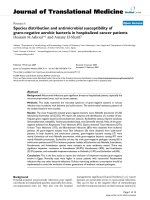
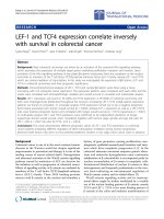
The study area included 5,625 km
2
of the Wind River
BasinincentralWyoming,USA(Figure1).Elevations
range from 1,478 to 2,776 m with variable topography
(gently sloping flats, cut banks, dry washes, steep slopes,
Webb et al. Ecological Processes 2012, 1:1
/>Page 2 of 15
and rocky canyons). Average maximum and minimum
temperature during the study period (April to July; here-
after nesting season) was 34.3°C and 10.8°C, respectively.
Total precipitation during the nesting season was 19.4
cm in 2008 (Fales Rock, WY, USA; s.dri.

edu/cgi-bin/rawMAIN.pl?wyWFAL), 12.0 cm in 2009,
and 12.6 cm in 2010. Weather data during the nesting
seasons of 2009 and 2010 were collected using Vantage
Figure 1 Study area of greater sage-grouse in central Wyoming. St udy area (5,625 km
2
) of female greater sage-grouse nest occurrence
(white dots) in the Wind River Basin of central Wyoming during 2008 to 2010. In 2010, there were 1,085 wells (black dots) associated with oil
and gas development. Background map represents probability of nest site occurrence within the landscape (adapted from Dzialak et al. 2011a).
Webb et al. Ecological Processes 2012, 1:1
/>Page 3 of 15
Pro2™ Precision Weather Stations (Davis Instruments
Corporation, Hayward, CA, USA) that were located cen-
trally within the study area (Figure 1).
Plants common to the area included Wyoming big
sagebrush (Artemisia tridentata subsp. wyomingensis),
basin big sagebrush (A. t.subsp.tridentata), mountain
big sagebrush (A. t.subsp.vaseyana and A. t.subsp.
pauciflora), little sagebrush ( A. arbuscula subsp. arbus-
cula), Patterson’s wormwood (A. pattersonii), black grea-
sewood (Sarcobatus vermiculatus), yellow rabbitbrush
(Chrysothamnus viscidiflorus), winterfat ( Ceratoides
lanata), shadscale saltbush (Atriplex confertifolia), lim-
ber pine (Pinus flexilis), and rocky mountain juniper
(Juniperus scopulorum) ( />The study area encompassed pre-existing and expand-
ing development of energy resources. Oil and natural
gas development was initiated in the 1920s, but gas
development has recently accelerated since the 1990s. In
2008, there were 1,002 wells associated with oil and gas
development in the study area. Wells increased 3.2%
from 2008 to 2009 (n = 1,034) and 4.9% from 2009 to

2010 (n = 1,085).
Capture and handling
During March and April of 2008 to 2010, we captured
sage-grouse on and around leks at night with the aid of
spotlights (Wakkinen et al. 1992). Capture also occurred
in autumn (September to November) to maintain sam-
ple size from dropped collars or fatalities. Females cap-
tured in autumn provided data during the nesting
season of the following year. We assigned age (yearling
< 2 years; adult ≥ 2 years) to each female based on the
appearance of primaries (Eng 1955; Crunden 1963), and
fitted sage-grouse with global positioning system [GPS]
collars (30-g ARGOS/GPS Solar PTT-100, Microwave
Telemetry, Inc., Columbia, MD, USA) using rump-
mounted techniques (e.g., Bedrosian a nd Craighead
2007). GPS collars had a 3- year operational life and
were configured with ultrahigh-frequency beacons for
ground tracking and detection of fatality. Collars were
programmed with two fix schedules: (1) one fix every 3
h from 0700 to 2200 hours during 16 February to 14
May and (2) one fix every hour during 15 May to 15
July. Animal capture and handling protocols were
approved by the Wyoming Game and Fish Department
(Chapter 33 Permit #649).
Nest monitoring
We used GPS locations (transmitted via ARGOS; www.
argos-system.org) to locate nests during egg-laying,
which has been found to provide a reliable and precise
estimation of nest initiation, incubatio n, and nest hatch
or failure (Dzi alak et al. 2011a). First, we examined the

spatial pattern of movement by the female during egg-
laying, which is characterized by brief visits of < 3 h to
a spatially distinct lo cation (i.e., nest site) every 2 to 3
days for a 9- to 12-day period (Schroeder et al. 1999).
Next, we observed that the female was e xclusively (or
almost exclusively) at the nest location for a complete
diel cycle on the first day of incubation. Thus, we used
this date as the initiation date of incubation.
We projected the expected hatch date using the aver-
age incubation period of 27 days from the first day of
incubation (Schroeder et al. 1999). If a female vacated
the nest site > 4 days prior to the projected hatch date,
we assumed that the nest was abandoned or failed, and
a field crew checked the status of the nest to determine
fate (date of first departure used as failure date).
We considered nests successful if ≥ 1egghatched;
otherwise, we classified the nest as unsuccessful, noting
the date and the age of the nest at failure and assigning
a cause of failure (i.e., depredated, other or unknown,
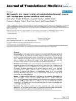
and death of female). Successfully hatched eggs (Figure
2) were identified by the presence of a distinct egg cap
and an intact egg membrane (initial cracking, or pip-
ping, of the egg typically results in two eggshell frag-
ments, with the smaller fragment called the cap); such
features are not typical of depredated e ggs (Figure 3;
Sargeant et al. 1998).
The spatial data (GPS locations transmitted via
ARGOS) allowed us to estimate with high probability
the first day of incubation and the date of nest failure or
hatch.Last,wewereabletomonitortheneststatuson

a daily schedule with GPS data that a llowed a straight-
forward means of modeling DSR of nests (see below).
This was an advantage compared to previous studies
that conducted periodic checks for nests, discovered
nests at various stages, estimated failure date because
nests were only periodically rechecked, and used an
exponent to account for survival across differing interval
lengths (i.e., logistic-exposure model; Shaffer 2004).
Spatial variables: landscape
Processes on the landscape occur and interact at multi-
ple spatial scales (Wiens 1989), and like ly carry-over t o
influence predator behavior on the landscape because
most predators also perceive the landscape at various
spatial scales (Chalfoun et al. 2002; Stephens et al.
2005). For these reasons, we use a multi-scalar approach
to examine the relationships between DSR of nests and
spatial landscape features (i.e., anthropogenic and land-
scape features, and t opography) important to sage-
grouse during nesting.
At the nest site (i.e. , 15-m spatial scale), we measured
shrub canopy and sagebrush canopy coverage using line
intercept methods (Canfield 1941). We stretched two
15-m tapes perpendicular to each other using the nest
site as the center point (i.e., 7.5 m on each tape); the
Webb et al. Ecological Processes 2012, 1:1
/>Page 4 of 15
direction of the first line was randomly determined, and
the second line was placed perpendicular to the first.
From the center point (i.e., the nest site), all shrub spe-
cies intersecting the transect lines were recorded to spe-

cies along the 7.5-m section of the line in each
direction. Gaps in shrub canopy of ≥ 5cmwerenot
recorded. We also m easured the percentage of herbac-
eous vegetation (grass, forbs, and total herbaceous vege-
tation) canopy coverage using 20 × 50-cm Daubenmire
plots (Daubenmire 1959). Daubenmire plots were placed
along each 15-m line at 1.5-m intervals, which finally
resulted in 20 plots. Last, we recorded the species of the
shrub within which the nest was located, along with the
height (in centimeters) of the shrub.
At larger spatial scales (i.e., ≥ 30 m; see below), we
used a geographic information system (ArcGIS
®
10.0,
Environmental Systems Research Institute, Inc., Red-
lands, CA, USA) to map anthropogenic and landscape
features, and topography because these features were
known to influence resource selection of sage-grouse
(Aldridge and Boyce 2007; Doherty et al. 2008; Dzialak
et al. 2011a). Four covariates depicted predominant
human modifications of the landscape, distance (in
meters) to the nearest oil or gas well, road, residential
structure, and energy-related ancillary feature. Data on
wells were current through July 2010 and were obtained
from the Wyoming Oil and Gas Conservation Commis-
sion ( We considered the
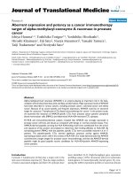
Figure 3 Photographs of depredated greater sage-grouse eggs. Photographs depicting depredated eggs by various nest predators. Patterns
are consistent with depredation and not a successful hatch (cf Figure 2b). Photographs courtesy of Chad V. Olson and Hayden-Wing Associates,
LLC.
Figure 2 Photographs of intact greater sage-grouse eggs and successfully hatched eggs. Photographs of an intact nest after it was

abandoned to show general nest site-specific vegetation features (a) and eggshells depicting a successful hatch based on pecking and eggshell
fragment patterns (b). Photographs courtesy of Chad V. Olson and Hayden-Wing Associates, LLC.
Webb et al. Ecological Processes 2012, 1:1
/>Page 5 of 15
distance to the nearest well during the year of nesting as
well as the distance to wells 1 and 2 years prior to nest-
ing (lag effects; Harju et al. 2010). Roads (paved,
improved, and dirt), structures, and ancillary features
(e.g., compressor stations, settling ponds, and buildings)
were heads-up digitized (1:500 to 1:2,000 scale) using
National Agriculture Imagery Program aerial photogra-
phy (1-m resolution).
We mapped five landscape features that depicted pre-
dominant vegetation in the study area: percentage (in
percent) of sagebrush, shrub, bare ground, litter, and
herbaceous vegetation (grass and forbs). We exami ned
these five landscape features at four spatial scales (num-
ber of 3 0-m pixels per side aro und the nest site, which
was located in the center cell); 30 m (1 × 1), 90 m (3 ×
3), 810 m (27 × 27), and 1,590 m (53 × 53). The 30-m
pixel represented the percentage of each variable and
was mapped across the landsca pe using the Provisional
Remote Sensing Sagebrush Habitat Quantification Pro-
ducts for Wyoming database, which was developed by
the United States Geological Survey (Homer et al. 2010).
Larger spatial scales (i.e., 90, 810, and 1,590 m) allowed
us to calculate an average percentage of each variable
around the nest site.
Last, we mapped five covariates that d epicted topogra-
phy and other natural features: elevation (in meters), heat

load index (Dzialak et al. 2011a), slope (in percent), terrain
roughness (standard deviation [SD] of elevation), and dis-
tance (in mete rs) t o m esic a reas. Elevation, slope, and
terrain roughness were generated using a 10-m digital ele-
vation model [DEM]. Slope was measured in degrees, and
terrain roughness was calculated as the SD of elevations
from the DEM at 90-, 810-, and 1,590-m scales. We calcu-
lated the distance to the nearest mesic area, whic h
included streams, seeps, springs, impoundments, irrigated
areas, and water discharge sites; the type of mesic area was
developed using Feature Analyst
®
4.2 (Visua l Learning
Systems, Inc., 2008) for ArcGIS
®
9.3 (ESRI, Redlands, CA,
USA). We used Spatial Analyst in ArcGIS
®
10.0 to calcu-
late raster values and to extract values from raster data to
location data f or all covariates. See Visual Learning
Systems, Inc. (2008) and Webb et al. (2011) for details on
using Feature Analyst, and Dzialak et al. (2011a) for a
more complete description of covariates, data sources, and
methods.
Nonspatial variables: weather
We also considered that nonspatial variables such as
weather may facilitate predators in finding nests because
weather factors such as temperature, moisture, and air
movements influence scent production as well as detec-

tion (Gutzwiller 1990). We obtained daily readings for
maximum, minimum, and average temperatures (in
degree Celsius); humidity (in percent); average and
maximum wind speeds (in kilometers per hour); and
precipitation (Conover 2007; Moynahan et al. 2007;
Conover et al. 2010; Dritz 2010); precipitation was con-
verted to a binomial variable that indicated the presence
or absence of rainfall ≥ 0.025 cm. The aforementioned
weather variables likely facilitate or inhibit olfa ction in
predators while searching for a prey. During nesting sea-
sons of 2009 and 2010, we installed and used weather
stations (Vantage Pro2™ Precision Weather Station,
Davis Instruments, Hayward, CA, USA) that were
locatedcentrallywithinthestudyarea(Figure1).We
installed centrally loca ted weather stations after the
nesting season of 2008; therefore, we did not have cen-
trally located weather data during 2008. However, dur-
ing 2008, we obtained nearby weather data from the
Western Regional Climate Cen ter (Fales Rock, WY,
USA; />wyWFAL); this station was 6.4 km south of our study
area (Figure 1).
Model development and analysis
Two additional variables were modeled: t he Julian date
and the age of the nest. The Julian date was modeled
because nest survival may be related to when the nest
was initiated. Simila rly, the age of the nest (number of
days since incubation began) was modeled to examine
whether nests e arly or late in incubation had a greater
probability of surviving. Before implementing a hierarch-
ical variable selection approach, we created quadratic

terms (quadratic = original
2
) for the following: the Julian
date (first day o f incubation); age of the nest (days since
incubation began); temperature; humidity; wind speed;
shrub height; percentage of bare ground, litter, forbs,
grass, total herbaceous vegetation, sagebrush, and shrub;
terrain roughness; elevation; and slope at all spatial
scales examined. We developed quadratic terms because
animals often avoid the lowest and highest values asso-
ciated with a given landscape feature (Aldridge and
Boyce 2007; Johnson et a l. 2004; Stephens et al. 2005;
Dzialak et al. 2011a). We also natural log-transformed
all distance variables (i.e., distance to wells, structures,
ancillary features, roads, and mesic habitat) to allow for
a decreasing magnitude of influence with increasing dis-
tance. To assure that a natural log transformation [ln]
was not attempted on a cell with a value = 0, we added
0.1 to all original values (new = ln(original + 0.1)). Last,
we created a new precipitation variable that indicated
whether precipitation occurred 1 day prior (i.e., a lag
event).
We implemented a four-step hierarchical variable
inclusion approach to reduce the number of variables in
the final model. First, we used an information-theoretic
approach (Burnham and Anderson 2002) to evaluate
each landscape variable at multiple spatial scales (e.g.,
Webb et al. Ecological Processes 2012, 1:1
/>Page 6 of 15
nest site (15-m scale), 30, 90, 810, and 1,590 m). We

selected the spatial scale and term for each landscape
variable using Akaike’ s information crit erion [AIC]
adjusted for small sample size [AICc] (Burnham and
Anderson 2002). We retained the spatial scale and term
for each variable with the lowest AICc. We used gener-
alized linear mixed models [GLMM] (PROC GLIMMIX,
SAS
®
9.2, SAS Institute Inc., Cary, NC, USA) and the
Laplace method of approximating the log likelihood to
determine the most appropriate spatial scale and term
for each landscape va riable (Appendix 1). Dat a were
analyzed using a logistic regression framework where
nest fate (survived or failed) on each day was analyzed
as a binary response variable (1 = survived; 0 = failed);
modeling daily nest fate as a binary response was the
basis for estimating the probability of daily nest survival
(i.e., DSR of nests). We included three random effect
statements to model the hierarchical structure of the
data set (Appendix 1). Random effects were used to
model the fate of nests because nest fates may be corre-
lated within (1) nesting attempts and individual birds
(nest identification ‘nested’ within bird identification;
NID(BIRD)), (2) individuals and years (bird identifica-
tion ‘nested’ within year; BIRD(YEAR)), and (3) years
(Appendix 1). We used a binary distribution, a logit-link
function (constraining DSR of nests between 0 and 1),
and a variance components-covariance structure for ran-
dom effects (Appendix 1). Second, after only one spatial
scale and term was selected for each landscape variable,

we assessed the correlation among remaining landscape
variables using PROC CORR (SAS
®
9.2; SAS Institute
Inc.) and eliminated covariates for r ≥ 0.5; the variable
providing the simplest biological interpretation was
retained. Third, we considered the remaining variables
to comprise a ‘full’ landscape model. Using the GLMM
described above, we assessed the influence of all covari-
ates in the full landscape model simultaneously on daily
nest fate (binary response variable) to estimate the prob-
ability of DSR of nests. We removed any variable where
P > 0.1, thus creating a reduced model for the last step
in building the most parsimonious final model of DSR
of nests. Last, we added weather variables to the final
landsca pe model to determine if the addition of weather
variables improved model fit (sensu Dinsmore et al.
2002). Thus, we refer to the final landscape model as a
null model f or assessing additional model building. We
considered only models with AICc values lower than the
null landscape model or within 2 ΔAICc units of the
null landscape model. Weather variables that resulted in
lowerAICcvalueswerecombinedtocreateamodel
with multiple weather variables. We also assessed the
relative plausibility of models in the set of candidate
models using Akaike weights [w
i
], with the best model
having the highest w
i

(Burnham and Anderson 2002).
We built the landscape model first because female
greater sage-grouse can make decisions on nest site
location and structure to aid in concealment from pre-
dators. Howe ver, weather is an uncontrollable influence
on nest fate that may facilitate predation; thus, these
variables were added last to assess their strength on
influencing DSR of nests.
Results
During the 3-year study, we monitored 83 nests initiated
by 67 individual females (Table1).Onefemalewas
killed while off the nest (approximately 600 m from the
nest as determined by GPS locations), whereas all others
were killed while on the nest. We analyzed data on the
one female that was killed approximately 600 m from
the nest because inclusion of this bird did not change
the magnitude or direction of the relationships with
landscape covariates.
We were interested only in DSR of nests during incu-
bation, so we excluded four nests that failed during egg-
laying and one nest that survived to 27 days, but was
considered unsuccessful because no eggs hatched. Of
the four birds that had a failed nest during egg-laying,
three birds incubated on their second attempt whereas
the remaining bird initiated two incubation attempts
after the failed egg-laying attempt.
Considering only incubation attempts of the 67 indivi-
dua l females, 14 females attempt ed a second nest and 2
females attempted to incubate three nests within a sea-
son. Ten incubation attempts were unsuccessful for

both the first and second attempts (71.4%; 10 of 14),
while four second attempts were successful after an
Table 1 Sample sizes and nest fates of greater sage-grouse in central Wyoming
Sample size
a
Dates
b
Nest fate
a
Apparent survival
c
Year Females Nests First Last Hatched Depredated Other Hen-killed
2008 17 18 26 April 11 June 5 13 0 0 0.28
2009 23 26 22 April 14 June 8 15 1 2 0.31
2010 27 39 21 April 12 July 11 22 0 6 0.28
Total 67 83 - - 24 50 1 8
¯
x
= 0.29
a
Annual sample sizes of female greater sage-grouse and nests, and corresponding nest fates, on the 5,625-km
2
study area in the Wind River Basin in central
Wyoming, USA.
b
Dates listed are for the initiation of the first nest (i.e., First) and the hatching or depredation of the last nest (i.e., Last). Nests of female greater
sage-grouse that died during incubation were considered failed nests.
c
Apparent annual nest survival (i.e., successful hatch) was calculated as ‘Hatched’ /’Nests.’
Webb et al. Ecological Processes 2012, 1:1

/>Page 7 of 15
unsuccessful first attempt (28.6%; 4 of 14). The two
females that attempted to incubate three nests were suc-
cessful during the third attempt. The earliest incubation
date was 21 April, and the latest date of nest failure or
hatch was 12 July (Table 1).
Average apparent nest survival was 28.9% (24 of 83)
and ranged from 0.28 to 0.31 during the three nesting
seasons (Table 1). Nest predation was t he most signifi-
cant form of mortality (84.7 %; 50 of 59) followed by
direct predation of the female (13.6%; 8 of 59) that
resulted in nest failure and other sources of nest
destruction (1.7%; 1 of 59; Table 1). In total, predation
accounted for 98.3% of nest failures.
Selection of specific covariates for each class of land-
scape, topographic, and anthropogenic variables revealed
that site-specific covariates were the most important
(i.e., ≤ 30 m), except for roughness, which was the most
important at the largest spatial scale examined (i.e.,
1,590 m; Table 2). Although we did not model the type
of shrub species at the nest site, we did observe that
nests were built under four species of shrubs: big sage-
brush species (76.2%), little sagebrush (13.6%), yellow
rabbitbrush (8.1%), and greasewood (2.1%). After remov-
ing correlated covariates and variables not important i n
the landscape mode l (P > 0.1), we retained two land-
scape covariates (percentage of shrub cover at nest site
(15-m scale) and distance to mesic habitat) and two
anthropogenic covariates (distance to oil and gas wells
anddistancetoroads;Table2).Wealsoretainedthe

date of initiation of the incubation process (Julian date)
and the nest age in the model (Table 2). The final land-
scape model thus included seven covariates, including
the intercept.
We used the final landscape model as the null model
from which to base the influence of weather variables
when added to the model. We found that adding
weather variables resulted in six m odels with a lower
AICc (n = 2) or within 2 AICc units of the null model
(n = 4; Table 3). The best model for daily nest survival
included 10 parameters and had a model weight of
0.774, which was 10.5 times more likely to be the best
approximating model compared to the next best model
(w
i
= 0.074; Table 3). All other models had w
i
≤ 0.053
(Table 3). Therefore, we considered only the best model
when calculating coefficient estimates and for plotting
relationships between DSR of nests and the covariates.
The Pearson chi-square statistic divided by degrees of
freedom indicated that models were specified reasonably
(0.66 to 1.03; Table 3).
ThelogisticregressionequationforDSRofnests
using the best model (see Table 3) was (standard error
[SE] reported in parentheses after the coefficient
estimate):
logit(


S
) = -3.3181(2.0704) + 0.0052(0.0112) × julian date
- 0.0559(0.0498) × age of n est + 0.0027(0.0229) × p ercentage
of shrubs + 0.6882(0.3052) × ln distance to wells - 0.0001
(0.0001) × distance to roads + 0.2813(0.1639) × ln distance
to mesic habitat + 0.0178(0.0287) × max wind speed -
0.0004(0.0003) × max wind speed
2
-0.7551(0.3167) × 1-day
lag in preci pitation (0 = no rain; 1 = ra in ≥ 0.025 cm).
Table 2 Variables considered important to greater sage-
grouse nest survival in central Wyoming
Variable Covariate Scale
(m)
Vegetation
Shrub height (-) Height of shrub (cm) at nest
a
15
b
Bare ground (-,
+)
Percentage (%) of bare ground
c
30
d
Litter (-, +) Percentage (%) of litter
c
30
Forbs (+) Percentage (%) of forb cover
a

15
Grass (-) Percentage (%) of grass cover
a
15
Total
herbaceous (-)
Percentage (%) of total herbaceous
cover
a
15
Sagebrush (-, +) Percentage (%) of sagebrush cover
c
15
Shrubs (+) Percentage (%) of total shrub cover
a
15
Mesic (+) Distance (m) to mesic habitat year of
nest
e
N/A
Topography
Elevation (-, +) Elevation (m)
c
30
Slope (+) Slope (%)
a
30
Roughness (+) Roughness index (SD of elevation)
a
1,590

d
Anthropogenic
Oil and gas
wells (+)
Distance (m) to wells year of nest
e
N/A
Structures (-) Distance (m) to structures year of nest
e
N/A
Ancillary
features (-)
Distance (m) to ancillary features year
of nest
e
N/A
Roads (-) Distance (m) to roads year of nest
a
N/A
Others
Initiation date
(+)
Julian date for first day of nest
incubation
a
N/A
Nest age (-) Age of nest (in days)
a
N/A
a

Linear term.
b
Refers to on-the-ground measurements of vegetation at the
nest site using either Daubenmire plots (forbs, grass, and total herbace ous
vegetation) or line transects (percentage of sagebrush and shrub canopy
cover).
c
Linear + quad ratic term.
d
Spatial scales depicted as an area (e.g., 30
or 1,600 m) using remotely sensed imagery and heads-up digitizing to
estimate variables.
e
Natural log-transform ed variable to allow for a decreasing
magnitude of influence with increasing distance. Variables selected from a
suite of variables at multiple spatial scales (the spatial scale for each variable
with the lowest AICc was retained) that were considered to influence nest
survival of female greater sage-grouse in the Wind River Basin in central
Wyoming, USA. Variables in italicized text were entered into a landscape
model after variable reduction based on AICc, correlation (PROC CORR; SAS
®
9.2), and non-significance (P > 0.1), and used as a null landscape model for
testing the influence of weather on daily nest survival. Signs (positive or
negative) in parentheses next to landscape variables represent the
relationship between the particular varia ble and the probability of DSR (when
two signs occur, the first represents the linear relationship and the second
represents the quadratic relationship). SD, standard devia tion; N/A, not
applicable.
Webb et al. Ecological Processes 2012, 1:1
/>Page 8 of 15

Overall DSR of nests was 0.95, resulting in an esti-
mated nest survival rate of 25.0%, while holding all cov-
ariatesconstantattheirmean values and considering a
1-day lag in precipitation. Average a pparent nest survi-
val (28.9%) was similar to the most parsimonious model
above (25.0%).
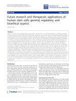
DSR was associated positively with the Julia n date
(Figure 4a), percentage of shrub cover (Figure 4b), dis-
tance to wells (Figure 4c), and distance to mesic habitat
(Figure 4d), but was associa ted negativ ely with nest age,
distance to roads, and maximum wind speed (Figure
4e). On average, females that successfully incubated a
clutch initiated incubation 5 days later (successful =
131.8 ± 2.9 SE; unsuccessful = 126.4 ± 1.5 SE), located
nests under greater shrub cover (successful = 23.7% ±
2.1 SE; unsuccessful = 18.8% ± 1.1 SE), were farther
from wells (successful = 4,445 m ± 656.8 SE; unsuccess-
ful = 3,353 m ± 440.4 SE) and mesic areas (successful =
1,060.2 m ± 119.0 SE; unsuccessful = 895.5 m ± 67.7
SE), but marginally closer to roads (successful = 2,568
m ± 615.2 SE; unsuccessful = 2,693 m ± 330.0 SE). Pre-
cipitation was analyzed as a binomial variable; thus, DSR
of nests was lower the day following precipitation events
of ≥ 0.025 cm. The relationships between DSR of nests
and distance to wells, distance to mesic habitat, and
maximum wind speed revealed thr esholds in the effect
of those variables on DSR of n ests. DSR of nests
increased significantly when placed 250 to 1,600 m from
the nearest oil or gas well (Figure 4c). In relation to the
distance from mesic habitat, DSR of nests was lowest

when the nest was within 50 m of the nearest mesic
area, leveling off after reaching the 50-m t hreshold (Fig-
ure 4d). Last, DSR of nests began to drop rapidly once
wind speeds reached or exceeded appro ximately 60 kph
(Figure 4e).
Discussion
In this st udy, we used the movement behavior of female
sage-grouse obtained from GPS collar data to identify
initiation of incubati on and subsequent failure or hatch-
ing of the nest. Unlike nest monitoring efforts based on
conventional telemetry, the approach we used allowed
nests to be monitored (1) remotely without observer
influence on incubation and (2) on a daily cycle, so the
exact date of nest hatch or failure was known. Based on
model weights (w
i
), there was little model uncertainty
(Burnham and Anderson 2002) as to the selection of the
best model among all candidate models. Within this
landscape, nest-site placement by female sage-grouse
was influenced by landscape variables at multiple spatial
scales (Dzialak et al. 2011a); however, DSR of nests was
most influenced by nest site-specific variables (area ≤ 30
× 30 m), similar to another study by Manzer and Han-
non (2005). This finding is in contrast to other studies
which found that landscape-level variables were most
influential on the success of nests by ground-nesting
birds (Stephens et al. 2005; Moynahan et al. 2007).
Examining the v ariables thatwereincludedinthefinal
model revealed potential mechanisms (i.e., visual and

olfa ctory) that predato rs used to locate nests when con-
sidering that nest depredation and direct predation of
the incubating female were the most common sources
of nest failure. Last, the modeling approach used offers
a simplified and unified framework for modeling n est-
and time-specific covariates, fixed and random effects,
complex hierarchical data str uctures, and multiple rela-
tionships (e.g., linear and quadratic) of the independent
var iables, and to account for the correlation of multiple
measurements on the same bird and nest (Appendix 1).
Female movement and activity, collected using GPS
collars, allowed researchers to find all nests beginning
on day 1 of incubation, a phenomenon that rarely
occurs in field studies (Shaffer 2004). This approach
offered several advantages. First, we reduced any con-
founding effects of nest age because all nests were
found and observed starting on day 1 of incubation (see
Dinsmore et al. 2002 for a discussion on nest age as a
confounding effect). Typica lly, apparent estimates of
Table 3 Model selection results that describe DSR of greater sage-grouse in central Wyoming
Model K AICc ΔAICc w
i
From the best From the null
Landscape + max wind (linear) + max wind (quadratic) + precipitation (1-day lag) 10 470.29 0 -5.36 0.774
Landscape + max wind (linear) + max wind (quadratic) 9 474.98 4.69 -0.67 0.074
Landscape 7 475.65 5.36 0 0.053
Landscape + max wind (linear) 8 476.96 6.67 1.31 0.028
Landscape + average wind (linear) + average wind (quadratic) 9 477.10 6.81 1.45 0.026
Landscape + average wind (linear) 8 477.24 6.95 1.59 0.024
Landscape + precipitation (1-day lag) 8 477.46 7.17 1.81 0.021

Model selection results for the best approxim ating model of DSR of nests for female greater sage-grouse in the Wind River Basin in central Wyoming, USA. Model
selection was based on ΔAICc using the landscape mode l (see Table 2) as the null model from which to base model fit with the addition of weather variables.
Only models ≤ 2 ΔAICc units from the null landscape model are reported, unless AICc was lower than the null landscape model. K, number of parameters in
model; AICc, Akaike’s information criterion corrected for small sample size; w
i
, Akaike weights; max, maximum .
Webb et al. Ecological Processes 2012, 1:1
/>Page 9 of 15
nest survival are biased (Moynahan et al. 2 007), but
under the conditions of equal detection probability
between active and inactive nests (those that have
already failed), apparent nest survival is relatively
unbiased (Shaffer 2004), as we saw from our estimates.
Therefore, we reduced the bias of estimates of nest sur-
vival because we found all nests (once incubation was
initiated) before they had a chance to fail. Second, we
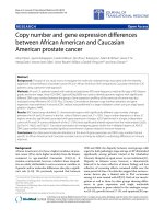
Figure 4 Probability of daily nest survival of greater sage-grouse relative to independent variables. Relationships between the probability of
daily nest survival (y-axis) for female greater sage-grouse in the Wind River Basin in central Wyoming, USA and independent variables (x-axis): (a)Julian
date (first day of incubation), (b) percentage (in percent) of shrub cover at the nest site (15-m scale), (c) distance (in meters) to the nearest oil or gas
well (distance variable was natural log-transformed), (d) distance (in meters) to mesic habitat (distance variable was natural log-transformed), and (e)
maximum wind speed (in kilometers per hour; data was fit using a quadratic term for wind speed). Maximum wind speed was recorded on the day of
nest failure. The x-axis is scaled to the range of observed values. Numbers next to arrows on each figure represent the probability of nest survival at
minimum and maximum values when extrapolated across the entire nesting season (i.e., twenty-seven 1-day intervals).
Webb et al. Ecological Processes 2012, 1:1
/>Page 10 of 15
modeled true DSR (interval = 1 day). Because we mod-
eled true DSR, time-spec ific covariates, such as weather,
were estimated with high precision (Shaffer 2004).
Third, observer disturbance was minimized, thereby
reducing this potentially confounding factor as a source

of nest failure. Fourth, most previous studies used very-
high-frequency transmitters to locate birds on nests
with variable search schedules, thereby finding nests
after the first day of incubation and thus biasing esti-
mates of survival high because nests failing early were
not detected. Crawford et al. (2004) reported an average
nest survival (defined as the probability of hatching ≥ 1
egg) rate of 47.4% (n = 14 studies). Potentially then, the
aforementioned average nes t survival estimate could be
biased high. Thus, our estimate of nest survival (25%)
may be more accurate, albeit lower, because nests were
detected on day 1 of incubation. Last, even when nests
are rechecked periodically, the GLMM approach we pre-
sent can still account for variable time intervals by using
methods (i.e., the link function contains an exponent (1/
t,wheret = len gth of observatio n interval) in the
numerator and denominator) similar to the logistic-
exposure model (see Equation 2 in Shaffer 2004).
Other researchers hypothesized that DSR of nests
would be lower in the early stages of incubation
becausevulnerablenestswouldbedepredatedearlier
(Klett and Johnson 1982; Coates and Delehanty 2010);
thus, we incorporated a time-dependent covariate (e.g.,
nest age) into models. However, we observed the
opposite trend; nests had a higher probability of daily
survival during early stages of incubation compared
with later stages of incubation. This finding supports
the idea that predators develop search images whereby
predators may learn to cue in on female behavior dur-
ing the course of incubation. Female attendance (Cao

et al. 2009) or activity (Burhans et al. 2002) at the nest
might draw the visual attention of predators to the site
of the nest. More specifically, nests failing later in
incubationmaysimplyberelatedtotheriskassociated
with exposure (Grant et al. 2005) where eggs exposed
totheriskforlongerperiodswillhavemoretimeto
be detected and depredated. It is also plausible that
the relationship between DSR of nests and nest age
could be a function of predators cuing in on the nest
duetoolfactionfromthefemale(Storaas1988)
because more odor will be emitted and bound to nest
substrates (Conover 2007) the longer a female remains
in one area (i.e., nest site).
In this study, there were several landscape features
that influenced DSR of nests, particularly nest site-speci-
fic variables (≤ 30 m). Most of these features interacted
with predator behavior to reduce or facilitate depreda-
tion of the nest. These features are important to con-
sider because nest failure in most avian species,
particularly ground-nesti ng birds, is due primarily to
predation (Gregg et al. 1994; Conway and Martin 2000;
Chalfoun et al. 200 2; Holloran et a l. 2005; Stephens et
al. 2005; Moyn ahan et al. 2007), as it was in th is study.
The amount (i.e., percentage) of shrub cover around the
nest site was important for reducing depredation. Sage-
brush (Artemisia spp.) was the primary brush species
comprising shrub canopy cover in our study, and it is
well known that the amount or height of sagebrush
around nest sites of sage-grouse is important for survival
(Connelly et al. 1991; Schroeder et al. 1999; Coates and

Delehanty 2010). DSR of nests increased linearly in rela-
tion to canopy cover of shrubs at the nest site. The
positive relationship observed in this study offers sup-
port that shrubs can provide physical impediments to
the nest. In addition, shrubs can serve as screening
cover to reduce visual detection by terrestrial predators
and canopy cover to reduce depredation by aerial preda-
tors. In general, greater concealment at the nest site
leads to a lower probability of nest discovery by vision-
based predators (Lima 2009). Thus, shrubs function pri-
marily as a visual impediment t o most predators of
nests, albeit shrubs also canfunctiontocreateturbu-
lence (measu re of varian ce of wind speed and direction)
and reduce the odor plume of the bird nesting within
(Conover 2007).
Although nest depredation often is a function of visual
detection of the nest or the incubating female by preda-
tors, we also indirectly considered the importance of
olfaction by terrestrial mammals while searching for
nests (Conover 2 007; Conover et al. 2010; Dritz 2010).
Similar to Moynahan et al. (2007), DSR of nests
decreased the day a fter a rainfall event. Higher failure
rates the day following precipitation events may have
been caused by a combination of factors. First, female
activity may have increased the day following precipita-
tion as the result of reduc ed activity (i.e., greater atten-
dance at the nest site) on the day of precipitation
(Moynahanetal.2007).Increasedactivityofthefemale
on the day following precipitation could have drawn
attention to the female or the nest by predators. Other

possible explanations include (1) increased predator
activity the day after precipitation events (Moynahan et
al. 2007) due to reduced activity on the days of precipi-
tation, and (2) high moisture contents in the air may
have facilitated olfaction of predators (Gutzwiller 1990)
that led them to the nest. For instance, a wet bird
releases more scent than a dry bird because water mole-
cules displace s cent molecules on the skin and feathers
and allow them to ev aporate and enter the air column
(Conover 2007). Therefore, it appears reasonable that
moisture within the air can heighten the olfactory senses
of predators because of increased scent released by the
bird.
Webb et al. Ecological Processes 2012, 1:1
/>Page 11 of 15
A second weather variable (maximum wind speed),
when added to the landscape model, improved model
fit, providing further evidence of an olfactory cue used
by predators to locate the source (i.e., the nest) of the
scent. Wind speed influences olfaction of predators by
carrying the scent over longer distances, allowing preda-
tors to track to the source of the scent (i.e., nest site). It
has been h ypothesized that high wind speeds will dilute
odor plumes to undetectable levels or create odor
plumes that are more difficult for a predator to follow
(Conover 2007). However, in windy conditions, preda-
tors may require a consistent wind direction to navigate
to the source of the odor (i.e., the nesting bird). It is
interesting to note that the two weather variables most
responsible for olfaction were included into the final

models whereas temperature and humidity were not; a
similar finding was observed by Dritz (2010).
Thereisagrowingbodyofliteraturethatpoints
towards energy development as a factor in reduced
demographic performance in certai n species (e.g., Saw-
yer et al. 2009; Harju et al. 2010; Gilbert and Chalfoun
2011; Dzialak et al. 2011b) through means such as
increased risk, landscape fragmentation, and altered pre-
dator communities and animal behavior. Typically,
human-altered landscapes have a greater abundance of
predators (Kurki et al. 1997, Kurki et al. 1998; Manzer
and Hannon 2005), which is facilitated by inf rastructure
associated with wells that provide artificial perch sites
for avian predators or ambush cover and den sites for
terrestrial mammals (i.e., predator subsidization; Manzer
and Hannon 2005; Coates and Delehanty 2010).
Although predators will exploit human-altered land-
scapes, it may take several years for the full effects of
disturbance to cascade across the landscape and influ-
ence predator occurrence. Therefore, it will be impor-
tant to incorporate lag effects into model building to
assess demographic responses related to disturbance
that occurred in previous years. Harju et al. (2010) and
Walker et al. (2007 ) report effects of previous develop-
ment on population and breeding performance of sage-
grouse. Therefore, we can infer that disturbance alters
landscapes and subsequently influences predator search
behavior or efficiency (Stephens et al. 2005).
In a recent study, the risk of losing a nest before hatch
was most influenced by distance to mesic areas and

wells; distance to roads did not structure nest survival
(Dzialak et al. 2011a). We observed that DSR of nests
was marginally greater for birds that nested closer to
roads. However, the difference in distance to the nearest
road between successful (2,568 m) and unsuccessful
(2,693 m) birds was 125 m, which could be considered
biologically insignificant. Given that birds nested away
from roads in general (mean ≥ 2,568 m), the minimal
difference in distance to the nearest road between the
two groups (125 m) and the finding that roads did not
structure the risk of nest failure (Dzialak et al. 2011a)
provides further support of the importance of other fac-
tors in structuring DSR of nests in this ground-nesting
bird of conservation concern.
Many species of grouse select for habitats with mesic
areas nearby for various life-history phases (Walker et
al. 2007). We found tha t nest surviva l was lowest when
nests were within 50 m from mesic habitat. This rela-
tionship may be caused by the use of mesic habitat by
predators (Stephens et al. 2005; Walker et al. 2007),
many of which function as travel corridors, edge habitat,
or ambush sites for terrestrial predators (Winter et al.
2000 ). While mesic areas associated with anthropogenic
features of the landscape reduced nest survival (Dzialak
et al. 2011a), DSR of nests was reduced when in proxi-
mity to any mesic area, likely due to the functional habi-
tatvalueoftheareaforawidenumberofavianand
terrestrial predators. In other studies, taller vegetation
associated with mesic areas increased the number of
perch sites for avian predators, thus facilitati ng preda-

tion of nests by avian predators (Manzer and Hannon
2005 ). Althoug h any type of mesic area reduced DSR of
nests, careful attention should be paid to water dis-
charge associated with anthropogenic activities (e.g.,
agricul ture irrigati on, oil and gas extraction, and ranch-
ing), which would artificially create and inflate the num-
ber of mesic areas (example of predator subsidization).
Conclusions
Nest site-specific landscape variables most influenced
DSR of nests in this sagebrush-obligate species, the
greater sage-grouse. However, managing for microsite
landscape characteristics is difficult. Large-scale manage-
ment practices are readily implemented across the land-
scape; thus, predi ctive mapping of the landscape factors
responsible for nest survival (longer temporal scale than
DSR)maybemoreappropriateforapplyingmanage-
ment actions (Dzialak et al. 2011a). This management
action does not take away from the fact that microsite
characteristics are important to DSR of nests . Nest sites
are located in a broader landscape context, which sup-
ports earlier studies which found that predators selected
landscape chara cteristics (including hum an-altered
areas) at larger spatial extents (Chalfoun et al. 2002; Ste-
phens et al. 2005). This may lead to reduced DSR of
nests when nest sites are located within the larger land-
scape selected by predators or in landscapes where
human activity subsidizes predators. Therefore, preda-
tors appear to be the proximate cause of reduced DSR
of nests whereby predator senses, such as visual and
olfactory acuities, are heightened in certain landscapes

and under variable weather conditions. However, the
ultimate cause of nest failure may stem from alterations
Webb et al. Ecological Processes 2012, 1:1
/>Page 12 of 15
to the landscape that typically occur across large spatial
extents leading to subsidized predator communities or
decoupled selection decisions used during nest site
selection. Although weather patterns cannot be managed
per se, managers can use predictive mapping of spatial
attributes of the landscape and model seasonal nest sur-
vival by including weather patterns experienced over the
nesting period to predict annual tren ds of breeding
dynamics.
Appendix
Appendix 1
Statistical code used to analyze DSR of nests
Statistical analysis (SAS
®
9.2, SAS Institute Inc., Cary,
NC, USA) code was used to analyze DSR of nests of
female greater sage-grouse (C. urophasianus)inthe
Wind River Basin in central Wyoming, USA. The statis-
tical procedure (i.e., GLIMMIX) used was a GLMM cap-
able of modeling both fixed and random effects.
PROC GLIMMIX DATA = S G_DSR METHOD =
LAPLACE;/*Specifies using the Laplace method of
approximating the log likelihood*/
CLASS BIRD NID YEAR PRECIP LAG;/*Categorical
variables for individual birds (BIRD), nest identification
(NID), year (YEAR), and 1-day lag in precipitation (0 =

no rain; 1 = rain ≥ 0.0254 cm; PRECIPLAG)*/
MODEL STATUS (EVENT = ‘ 1’ )=JULIAN
NESTAGE SHRUBS WELL0LAG_LOG
DISTROAD DISTMESIC_LOG WINDMAXKPH
WINDMAXKPH_QUAD
PRECIPLAG/SOLU TION DIST = BINOMIAL LINK
= LOGIT CL;/*Status refers to whether the nest sur-
vived (event = 1) or failed (event = 0) the 1-day interval;
in this case we are modeling probability of survival
(event = 1)*/
/*What follows next are the independent variables that
can be either categorical or continuous, and either time-
constant (e.g., landscape variables such as percentage of
shrub canopy cover [SHRUBS], natural log-transformed
distance to oil and gas wells [WELL0LAG_LOG], dis-
tance to nearest road [DISTROAD], and natural log-
transformed distance to nearest mesic habitat [DISTME-
SIC_LOG]) or time-specific (e.g., weather variables such
as maximum wind speed [WINDMAXKPH] and a 1-day
lag in precipitation [PRECIPLAG])*/
/*Nest status was modeled as following a binomial dis-
tribution with a logit link function; the “ SOLUTION ”
option requests display of coefficient estimates and stan-
dard errors, and “CL” requests co nfidence limits on the
coefficient estimates for each independent variable*/
/*The following random statements model the hier-
archical structure of the data*/
RANDOM NID(BIRD)/TYPE = VC;/* Fates of nests
within each nesting attempt are “nested” within each
individual bird (i.e., nest f ates may be correlated within

individual birds); “TYPE = VC” models the correlation
among nests within birds using a variance components
covariance structure (this is the default in SAS but other
covariance structures can be specified). This means that
variance componen ts are modeled separately for each
random effect and are independent.*/
RANDOM BIRD(YEAR)/TYPE = VC;/*Fates of nests
within birds are “nested” within each year (i.e., nest fates
may be correlated within individual birds within each
year). For birds sampled in multiple years, nest fate may
be correlated within years for that bird but are assumed
independent among years.*/
RANDOM YEAR/TYPE = VC;/*Fates of nests may be
correlated within years. For example, due to weather,
some years may have high nest failure rates for all birds.
This accounts f or that fact to better estimate the effect
of other independent variables.*/
RUN;
Abbreviations
AIC: Akaike’s information criterion; AICc: Akaike’s information criterion
corrected for small sample size; DEM: digital elevation model; DSR: daily
survival rate; GLMM: generalized linear mixed model; GPS: global positioning
system; PTT: platform terminal transmitters; w
i
: Akaike weights.
Acknowledgements
Funding was provided by ConocoPhillips, EnCana Oil and Gas, and Noble
Energy. We thank S. Oberlie (Bureau of Land Management) and G. Anderson
(Wyoming Game and Fish Department) for the logistical support; the Lander
Sage-Grouse Working Group for providing six transmitters; C. Aldridge

(United States Geologic Survey) for providing remotely sensed sagebrush
habitat quantification products for Wyoming; J. Mudd for the GIS support; M.
Pollock for the early project input and data management; and J. Dinkins, C.
Hedley, and several anonymous reviewers for improving the early versions of
this manuscript. KC Harvey Environmental, LLC provided in-kind support to
DL during the drafting and revising of this manuscript. The commercial
funding sources were not involved with the design and development of the
research protocol; collection, analysis, or interpretation of data; the writing of
this manuscript; or the decision to submit this manuscript.
Author details
1
Hayden-Wing Associates, LLC, 2308 South 8th Street, Laramie, WY, 82070,
USA
2
KC Harvey Environmental, LLC, 376 Gallatin Park Drive, Bozeman, MT,
59715, USA
Authors’ contributions
SLW designed the study, managed and analyzed the data, wrote the
statistical code, and drafted the manuscript. CVO designed the study,
managed the data, and helped draft the manuscript. MRD designed the
study, provided statistical assistance, analyzed portions of the data set, and
helped draft the manuscript. SMH assisted in developing the statistical code
and in drafting the manuscript. JBW designed the study and reviewed the
manuscript drafts. DL designed the study, collected the field data, and
reviewed the manuscript drafts. All authors read and approved the final
manuscript.
Competing interests
This work was funded by commercial sources: ConocoPhillips, EnCana Oil
and Gas, and Noble Energy. Hayden-Wing Associates, LLC provided in-kind
contributions that included travel costs associated with the dissemination of

this work and materials associated with data collection and analysis such as
GPS devices and statistical analysis software. Havin g received funding from
commercial sources, the consultancy could reasonably be perceived as a
Webb et al. Ecological Processes 2012, 1:1
/>Page 13 of 15
financial competing interest. This does not alter the authors’ views or
adherence to journal policies on publishing original scientific findings. Last,
the commercial funding sources were not involved with the design and
development of the research protocol; the collection, analysis, or
interpretation of data; the writing of this manuscript; or the decision to
submit this manuscript.
Received: 6 September 2011 Accepted: 10 February 2012
Published: 10 February 2012
References
1. Aldridge CL, Boyce M (2007) Linking occurrence and fitness to persistence:
habitat based approach for endangered greater sage-grouse. Ecol Appl
17:508–526
2. Becker JM, Duberstein CA, Tagestad JD, Downs JL (2009) Sage-grouse and
wind energy: biology, habits and potential effects from development,
report number PNNL-18567. Pacific Northwest National Laboratory, Richland
3. Bedrosian B, Craighead D (2007) Evaluation of techniques for attaching
transmitters to common raven nestlings. Northwest Nat 88:1–6
4. Burhans DE, Dearborn D, Thompson FR III, Faaborg J (2002) Factors
affecting predation at songbird nests in old fields. J Wildl Manage
66:240–249
5. Burnham KP, Anderson DR (2002) Model selection and inference: a practical
information-theoretic approach. Springer, New York
6. Canfield RH (1941) Application of the line interception method in sampling
range vegetation. J For 39:388–394
7. Cao J, He CZ, Wells KMS, Millspaugh JJ, Ryan MR (2009) Modeling age and

nest-specific survival using a hierarchical Bayesian approach. Biom
65:1052–1062
8. Chalfoun AD, Martin TE (2009) Habitat structure mediates predation risk for
sedentary prey: experimental tests of alternative hypotheses. J Anim Ecol
78:497–503
9. Chalfoun AD, Thompson FR III, Ratnaswamy MJ (2002) Nest predators and
fragmentation: a review and meta-analysis. Conser Biol 16:306–318
10. Coates PS, Delehanty DJ (2010) Nest predation of greater sage-grouse in
relation to microhabitat factors and predators. J Wildl Manage 74:240–248
11. Connelly JW, Braun CE (1997) Long-term changes in sage grouse
Centrocercus urophasianus populations in western North America. Wildl Biol
3:229–234
12. Connelly JW, Wakkinen WL, Apa AD, Reese KP (1991) Sage grouse use of
nest sites in southeastern Idaho. J Wildl Manage 55:521–524
13. Conover MR (2007) Predator-prey dynamics: the use of olfaction. Taylor and
Francis, Boca Raton
14. Conover MR, Borgo JS (2009) Do sharp-tailed grouse select loafing sites to
avoid visual or olfactory predators? J Wildl Manage 73:242–247
15. Conover MR, Borgo JS, Dritz RE, Dinkins JB, Dahlgren DK (2010) Greater
sage-grouse select nest sites to avoid visual predators but not olfactory
predators. Condor 112:331–336
16. Conway CJ, Martin TE (2000) Evolution of passerine incubation behavior:
influence of food, temperature, and nest predation. Evolution 54:670–685
17. Crawford JA, Olson RA, West NE, Mosley JC, Schroeder MA, Whitson TD,
Miller RF, Gregg MA, Boyd CS (2004) Ecology and management of sage-
grouse and sage-grouse habitat. J Range Manage 57:2–19
18. Crooks KR, Soulé ME (1999) Mesopredator release and avifaunal extinctions
in a fragmented system. Nature 400:563–565
19. Crunden CW (1963) Age and sex of sage-grouse from wings. J Wildl
Manage 27:846–849

20. Daubenmire RF (1959) A canopy-coverage method of vegetation analysis.
Northwest Sci 33:43–64
21. Dinsmore SJ, White GC, Knopf FL (2002) Advanced techniques for modeling
avian nest survival. Ecology 83:3476–3488
22. Doherty KE, Naugle DE, Walker BL, Graham JM (2008) Greater sage-grouse
winter habitat selection and energy development. J Wildl Manage
72:187–195
23. Dritz RE (2010) Influence of landscape and weather on foraging by
olfactory meso-predators in Utah. Thesis, Utah State University
24. Dzialak MR, Olson CV, Harju SM, Webb SL, Mudd JP, Winstead JB, Hayden-
Wing LD (2011) Identifying and prioritizing greater sage-grouse nesting and
brood-rearing habitat for conservation in human-modified landscapes. PLoS
ONE 6(10):e26273. doi:10.1371/journal.pone.0026273
25. Dzialak MR, Webb SL, Harju SM, Winstead JB, Wondzell JJ, Mudd JP,
Hayden-Wing LD (2011) The spatial pattern of demographic performance as
a component of sustainable landscape management and planning. Landsc
Ecol 26:775–790
26. Eng RL (1955) A method for obtaining sage grouse age and sex ratios from
wings. J Wildl Manage 19:267–272
27. Gilbert MM, Chalfoun AD (2011) Energy development affects populations of
sagebrush songbirds in Wyoming. J Wildl Manage 75:816–824
2
8.
Grant TA, Shaffer TL, Madden EM, Pietz PJ (2005) Time-specific variation
in passerine nest survival: new insights into old questions. Auk
122:661–672
29. Gregg MA, Crawford JA, Drut MS, DeLong AK (1994) Vegetational cover and
predation of sage grouse nests in Oregon. J Wildl Manage 58:162–166
30. Gutzwiller KJ (1990) Minimizing dog-induced biases in game bird research.
Wildl Soc Bull 18:351–356

31. Harju SM, Dzialak MR, Taylor RC, Hayden-Wing LD, Winstead JB (2010)
Thresholds and time lags in the effects of energy development on greater
sage-grouse populations. J Wildl Manage 74:437–448
32. Holloran MJ, Anderson SH (2005) Spatial distribution of greater sage-grouse
nests in relatively contiguous sagebrush habitats. Condor 107:742–752
33. Holloran MJ, Heath BJ, Lyon AG, Slater SJ, Kuipers JL, Anderson SH (2005)
Greater sage-grouse nesting habitat selection and success in Wyoming. J
Wildl Manage 69:638–649
34. Homer CG, Aldridge CL, Meyer DK, Schell S (2010) Provisional remote
sensing sagebrush habitat quantification products for Wyoming. U.S.
Geological Survey, Sioux Falls
35. Johnson CJ, Seip DR, Boyce MS (2004) A quantitative approach to
conservation planning: using resource selection functions to map the
distribution of mountain caribou at multiple spatial scales. J Appl Ecol
41:238–251
36. Klett AT, Johnson DH (1982) Variability in nest survival rates and
implications to nesting studies. Auk 99:77–87
37. Kurki S, Helle P, Lindén H, Nikula A (1997) Breeding success of black grouse
and capercaillie in relation to mammalian predator densities on two spatial
scales. Oikos 79:301–310
38. Kurki S, Nikula A, Helle P, Lindén H (1998) Abundances of red fox and pine
martin in relation to the composition of boreal forest landscapes. J Anim
Ecol 67:874–886
39. Larivière S, Walton LR, Messier F (1999) Selection by striped skunks (Mephitis
mephitis) of farmsteads and buildings as denning sites. Am Midl Nat
142:96–101
40. Lima SL (2009) Predators and the breeding bird: behavioral and
reproductive flexibility under the risk of predation. Biol Rev 84:485–513
41. Lyon AG, Anderson SH (2003) Potential gas development impacts on sage
grouse nest initiation and movement. Wildl Soc Bull 31:486–491

42. Manzer DL, Hannon SJ (2005) Relating grouse nest success and corvid
density to habitat: a multi-scale approach. J Wildl Manage 69:110–123
43. Moynahan BJ, Lindberg MS, Rotella JJ, Thomas JW (2007) Factors affecting
nest survival of greater sage-grouse in northcentral Montana. J Wildl
Manage 71:1173–1783
44. Nams VO (1997) Density-dependent predation by skunks using olfactory
search images. Oecologia 110:440–448
45. Sargeant AB, Sovada MA, Greenwood RJ (1998) Interpreting evidence of
depradation of duck nests in the prairie pothole region. U.S. Geological
Survey Northern Prairie Wildlife Research Center, Jamestown
46. Sawyer H, Kauffman MJ, Nielson RM (2009) Influence of well pad activity on
winter habitat selection patterns of mule deer. J Wildl Manage
73:1052–1061
47. Schroeder MA, Young JR, Braun CE (1999) Greater sage-grouse (Centrocercus
urophasianus). In: Poole A (ed) The Birds of North America, No. 425. Cornell
Lab of Ornithology, Ithaca
48. Schroeder MA, Aldridge CL, Apa AD, Bohne JR, Braun CE, Bunnell SW,
Connelly JW, Deibert PA, Gardner SC, Hilliard MA, Kobriger GD, McAdam SM,
McCarthy CW, McCarthy JJ, Mitchell DL, Rickerson EV, Stiver SJ (2004)
Distribution of sage-grouse in North America. Condor 106:363–376
49. Shaffer TL (2004) A unified approach to analyzing nest success. Auk
121:526–540
50. Stephens SE, Koons DN, Rotella JJ, Willey DW (2003) Effects of habitat
fragmentation on avian nesting success: a review of the evidence at
multiple spatial scales. Biol Conser 115:101–
110
Webb et al. Ecological Processes 2012, 1:1
/>Page 14 of 15
51. Stephens SE, Rotella JJ, Lindberg MS, Taper ML, Ringelman JK (2005) Duck
nest survival in the Missouri Coteau of North Dakota: landscape effects at

multiple spatial scales. Ecol Appl 15:2137–2149
52. Storaas T (1988) A comparison of losses in artificial and naturally occurring
capercaillie nests. J Wildl Manage 52:123–126
53. United States Fish and Wildlife Service (2010) Endangered and threatened
wildlife and plants: 12-month finding for petitions to list the greater sage-
grouse (Centrocercus urophasianus) as threatened or endangered. Fed Reg
75:13910–14014
54. Visual Learning Systems, Inc (2008) Feature Analyst® 4.2 for ArcGIS®
reference manual. Visual Learning Systems, Inc., Missoula
55. Wakkinen WL, Reese KP, Connelly JW, Fischer RA (1992) An improved
spotlighting technique for capturing sage-grouse. Wildl Soc Bull 20:425–426
56. Walker BL, Naugle DE, Doherty KE (2007) Greater sage-grouse population
response to energy development and habitat loss. J Wildl Manage
71:2644–2654
57. Webb SL, Dzialak MR, Wondzell JJ, Harju SM, Hayden-Wing LD, Winstead JB
(2011) Survival and cause-specific mortality of female Rocky Mountain elk
exposed to human activity. Popul Ecol 53:483–493
58. Wiens JA (1989) Spatial scaling in ecology. Funct Ecol 3:385–397
59. Winter M, Johnson DH, Faaborg J (2000) Evidence for edge effects on
multiple levels in tallgrass prairie. Condor 102:256–266
doi:10.1186/2192-1709-1-4
Cite this article as: Webb et al.: Landscape features and weather
influence nest survival of a ground-nesting bird of conservation
concern, the greater sage-grouse, in human-altered environments.
Ecological Processes 2012 1:1.
Submit your manuscript to a
journal and benefi t from:
7 Convenient online submission
7 Rigorous peer review
7 Immediate publication on acceptance

7 Open access: articles freely available online
7 High visibility within the fi eld
7 Retaining the copyright to your article
Submit your next manuscript at 7 springeropen.com
Webb et al. Ecological Processes 2012, 1:1
/>Page 15 of 15