Accounting Workbook Cheat Sheet_9 doc
Bạn đang xem bản rút gọn của tài liệu. Xem và tải ngay bản đầy đủ của tài liệu tại đây (417.15 KB, 25 trang )
242
Part III: Managerial, Manufacturing, and Capital Accounting
11. Towards the end of the year, the president of Company Y looks at the preliminary numbers for
operating profit and doesn’t like what he sees. He’s “promised” the board of directors that operat-
ing profit for the year will come in at $4,850,000. In fact, his bonus depends on hitting that operat-
ing profit target. There is still time before the end of the year to crank up production output for
the year. Therefore, he orders that production output be stepped up. The president asks you to
determine what the production output level for the year would have to be in order to report
$4,850,000 operating profit for the year. Of course, you have ethical qualms about doing this, but
you need the job. So, you reluctantly decide to do the calculation. Determine the production
output level that would yield $4,850,000 operating profit for the year.
Solve It
12. Refer to your answer to Question 10, in which Company Z produces only 2,000,000 units during
the year. In the scenario shown in Figure 11-2, the business manufactures 2,500,000 units, which is
its maximum production output for the year. Do you think that Company Z cranked up production
output to 2,500,000 units mainly to boost its operating profit for the year?
Solve It
Calculating Product Cost in Unusual Situations
The basic calculation model for product cost is:
Total manufacturing costs for period ÷ Total units produced during period =
Product cost per unit
Total manufacturing costs for the period includes direct manufacturing costs that can be
clearly identified with a particular product and indirect manufacturing costs that are allo-
cated to the product.
17_791458 ch11.qxp 6/26/06 7:18 PM Page 242
More free books @ www.BingEbook.com
This product cost calculation method is appropriate in most situations. However, it has to be
modified in two extreme situations:
ߜ When manufacturing costs are grossly excessive or wasteful due to inefficient produc-
tion operations
ߜ When production output is significantly less than normal capacity utilization
Suppose that Company X had to throw away $1,200,000 of raw materials during the year
because they weren’t stored properly and ended up being unusable in the production
process. The manager in charge of the warehouse received a stiff reprimand.
243
Chapter 11: Manufacturing Cost Accounting
Q. In Figure 11-1, which shows Company X’s operating profit performance and summary of manufac-
turing activity for the year, it is assumed that there were no wasteful manufacturing costs. In
this question, assume, instead, that the business had to throw away $1,200,000 of unusable raw
materials. How should the $1,200,000 cost of raw materials that were thrown out be presented in
the operating profit report and summary of manufacturing activity?
A. The $1,200,000 cost of raw materials that were wasted and not used in production should not be
included in the calculation of product cost. The $1,200,000 cost of wasted raw materials should be
treated as a period cost, which means that it’s recorded as an expense in the period. The operating
profit report and summary of manufacturing activity for the year in this scenario is as follows:
Company X
Operating Profit Report For Year Per Unit Totals
Sales volume, in Units 110,000
Sales Revenue $1,400.00 $154,000,000
Cost of Goods Sold Expense (see below) (750.00) (82,500,000)
Gross Margin $650.00 $71,500,000
Variable Operating Expenses (300.00) (33,000,000)
Contribution Margin $350.00 $38,500,000
Fixed Operating Expenses (21,450,000)
Cost of Wasted Raw Materials (1,200,000)
Operating Profit $15,850,000
Manufacturing Activity Summary For Year Per Unit Totals
Annual Production Capacity, in Units = 150,000
Actual Output, in Units = 120,000
Raw Materials $205.00 $24,600,000
Direct Labor 125.00 15,000,000
Variable Manufacturing Overhead Costs 70.00 8,400,000
Total Variable Manufacturing Costs $400.00 $48,000,000
Fixed Manufacturing Overhead Costs 350.00 42,000,000
Product Cost and Total Manufacturing Costs $750.00 $90,000,000
The $1,200,000 wasted raw materials cost is recorded as an expense in the year, as you see
in the operating profit report. As a result, the cost of raw materials is reduced the same
amount in the manufacturing activity summary for the year with the result that product
cost drops to $750 per unit.
17_791458 ch11.qxp 6/26/06 7:18 PM Page 243
More free books @ www.BingEbook.com
244
Part III: Managerial, Manufacturing, and Capital Accounting
13. The president of Company X is puzzled by the operating profit report and summary of manufac-
turing activity for the year, in which $1,200,000 raw materials cost was wasted and charged to
expense in the year. He expected that operating profit would be $1,200,000 lower (as compared to
the scenario in Figure 11-1, in which there’s no wasted raw materials cost). Operating profit in the
wasted raw materials scenario is only $100,000 lower than in Figure 11-1. Explain to the president
why operating profit is only $100,000 lower.
Solve It
14. After Company Y’s operating profit report and summary of manufacturing activity for the year has
been prepared (see Figure 11-2), you, the chief accountant, learn that $1,000,000 of raw materials
were thrown away during the year because the items had spoiled and couldn’t be used in the
manufacturing process. The company’s president knows about this loss and insists that no
change be made in the operating profit report and summary of manufacturing activity. Do you go
along with the president, or do you argue for changing the operating profit report and summary of
manufacturing activity?
Solve It
17_791458 ch11.qxp 6/26/06 7:18 PM Page 244
More free books @ www.BingEbook.com
As I mention earlier, unused production capacity is called idle capacity. One argument is that
the cost of idle capacity should be charged off as a period cost (that is, charged directly to
expense in the year and not included in product cost). Generally, the cost of idle capacity is
calculated as follows:
Percent of idle capacity × Fixed manufacturing overhead costs = Cost of idle capacity
Refer to Company Y’s operating profit report and summary of manufacturing activity for the
year (Figure 11-2). Its annual production capacity is 800,000 units, but it produced only
500,000 units during the year. The company’s idle capacity is 37.5 percent. In this case, the
idle capacity cost is calculated as follows:
37.5 percent idle capacity × $8,000,000 fixed manufacturing overhead costs = $3,000,000
cost of idle capacity
245
Chapter 11: Manufacturing Cost Accounting
Q. How would Company Y’s operating profit report and summary of manufacturing activity be
revised if the cost of idle capacity is treated as a period cost in the year?
A. The $3,000,000 cost of idle capacity is taken out of fixed manufacturing overhead costs and moved
up to the operating profit report as an expense in the period. The revised operating profit report
and summary of manufacturing activity, which you may find somewhat surprising, is as follows:
Company Y
Operating Profit Report For Year Per Unit Totals
Sales volume, in Units 500,000
Sales Revenue $85.00 $42,500,000
Cost of Goods Sold Expense (see below) (50.00) (25,000,000)
Gross Margin $35.00 $17,500,000
Variable Operating Expenses (12.50) (6,250,000)
Contribution Margin $22.50 $11,250,000
Fixed Operating Expenses (5,000,000)
Cost of Idle Capacity (3,000,000)
Operating Profit $3,250,000
Manufacturing Activity Summary For Year Per Unit Totals
Annual Production Capacity, in Units 800,000
Actual Output, in Units 500,000
Raw Materials $15.00 $7,500,000
Direct Labor 20.00 10,000,000
Variable Manufacturing Overhead Costs 5.00 2,500,000
Total Variable Manufacturing Costs $40.00 $20,000,000
Fixed Manufacturing Overhead Costs 10.00 5,000,000
Product Cost and Total Manufacturing Costs $50.00 $25,000,000
17_791458 ch11.qxp 6/26/06 7:18 PM Page 245
More free books @ www.BingEbook.com
246
Part III: Managerial, Manufacturing, and Capital Accounting
Allocating indirect costs is as simple as ABC . . . not!
Most manufacturers make many different products. Just
think of General Motors or Ford and the number of dif-
ferent car and truck models they assemble. If a separate
production plant (building, machinery, equipment, tools,
workforce, and so on) were dedicated to making only
one product, all manufacturing costs would be
direct
costs to that one particular product. But in reality, it’s the
other way around: One production plant is used to make
many different products. The result is that many pro-
duction costs are
indirect
to the different products man-
ufactured by the business.
Indirect manufacturing costs are allocated among the
products produced during the period. Therefore, prod-
uct cost includes both direct and indirect manufacturing
costs. Coming up with a completely satisfactory alloca-
tion method is difficult and ends up being somewhat
arbitrary — but it must be done in order to determine
product cost.
Accountants have developed many methods and
schemes for allocating indirect overhead costs, many of
which are based on some common denominator of pro-
duction activity, such as direct labor hours. A different
method that has gotten a lot of press is called
activity-
based costing
(ABC).
With the ABC method, you identify each necessary, sup-
porting activity in the production process and collect
costs into a separate pool for each identified activity.
Then you develop a
measure
for each activity — for
example, the measure for the engineering department
may be hours, and the measure for the maintenance
department may be square feet. You use the activity
measures as
cost drivers
to allocate cost to products.
So if Product A needs 200 hours of the engineering
department’s time, and Product B is a simple product
that needs only 20 hours of engineering, you allocate ten
times as much of the engineering cost to Product A.
The idea is that the engineering department doesn’t
come cheap; including the cost of their slide rules and
pocket protectors as well as their salaries and benefits,
the total cost per hour for those engineers could be $150
to $200, or more. The logic of the ABC cost-allocation
method is that the engineering cost per hour should be
allocated on the basis of the number of hours (the driver)
required by each product. In similar fashion, suppose the
cost of the maintenance department is $20 per square
foot per year. If Product C uses twice as much floor
space as Product D, you charge it with twice as much
maintenance cost.
The ABC method has received much praise for being
better than traditional allocation methods, especially for
management decision-making. However, you should
keep in mind that it requires rather arbitrary definitions of
cost drivers, and having too many different cost drivers,
each with its own pool of costs, isn’t practical.
Managers should be aware of which cost allocation
methods are being used by their companies and should
challenge a method if they think that it’s misleading and
should be replaced with a better (though still somewhat
arbitrary) method. I don’t mean to put too fine a point on
this, but to a large extent, cost allocation boils down to
a “my arbitrary method is better than your arbitrary
method” argument.
Note that changing the handling of the cost of idle capacity produces no difference in the
company’s operating profit for the year. Is this surprising, or what? In this example, the
company produces the same number of units it sells during the year. Thus, there’s no
“inventory effect.” One-hundred percent of its manufacturing costs for the year end up in
expense regardless of the way in which the idle capacity is handled. In Figure 11-2, the
entire $8,000,000 fixed manufacturing overhead costs ends up in cost of goods sold expense.
In this example scenario, $3,000,000 of the fixed costs end up in a period expense account
(Cost of Idle Capacity), and the other $5,000,000 ends up in cost of goods sold expense.
17_791458 ch11.qxp 6/26/06 7:18 PM Page 246
More free books @ www.BingEbook.com
247
Chapter 11: Manufacturing Cost Accounting
15. Assume that Company Z manufactures 2,100,000 units during the year (instead of the 2,500,000
units production output shown in Figure 11-2). Determine its operating profit for the year. Assume
that the cost of idle capacity is treated as a period cost and isn’t embedded in product cost.
Solve It
16. Refer to Company X’s operating profit report and summary of manufacturing activity presented in
Figure 11-1. Note that its annual production capacity is 150,000 units, but the business manufac-
tured only 120,000 units during the year. Therefore, it had 20 percent idle capacity (30,000 units
not produced ÷ 150,000 units production capacity = 20 percent idle capacity). However, the cost of
idle capacity isn’t treated as a separate period cost; all the company’s fixed manufacturing over-
head costs are included in calculating its product cost.
Suppose that the business treats the cost of idle capacity as a period cost. Prepare a revised oper-
ating profit report and summary of manufacturing activity for the business.
Solve It
17_791458 ch11.qxp 6/26/06 7:18 PM Page 247
More free books @ www.BingEbook.com
248
Part III: Managerial, Manufacturing, and Capital Accounting
Answers to Problems on Manufacturing
Cost Accounting
The following are the answers to the practice questions presented earlier in this chapter.
a
The company’s total manufacturing costs for the year are $91,200,000 (see Figure 11-1), but only
$83,600,000 is charged to cost of goods expense. What happened to the other $7,600,000
($91,200,000 manufacturing costs for year – $83,600,000 cost of goods sold expense for year =
$7,600,000)?
The business produced 120,000 units, which is 10,000 more units than the 110,000 units it sold
during the year. Therefore,
1
⁄12 (10,000 ÷ 120,000) of its total manufacturing costs is allocated to
the increase in inventory, and 11/12 is allocated to cost of goods sold during the year:
11
⁄12 × $91,200,000 total manufacturing costs = $83,600,000 allocated to cost of goods sold
expense
1
⁄12 × $91,200,000 total manufacturing costs = $7,600,000 allocated to inventory
You can also answer this question by using product cost and number of units sold during
the year:
$760 product cost × 110,000 units sold during year = $83,600,000 cost allocated to cost of
goods sold expense
$760 product cost × 10,000 units increase in inventory = $7,600,000 cost allocated to
inventory
b
As you can see in Figure 11-1, Company X recorded $42,000,000 fixed manufacturing overhead
costs in the year. Suppose, instead, that its fixed manufacturing overhead costs were $45,600,000
for the year, which is an increase of $3,600,000. Would the company’s operating profit have been
$3,600,000 lower? (Assume that variable manufacturing costs per unit and operating expenses
remain the same.)
No, operating profit would not be $3,600,000 lower. The following schedule shows that operat-
ing profit would be $3,300,000 lower. The higher fixed manufacturing overhead costs drive up
the product cost per unit, from $760 to $790, or $30 per unit. However, the business sold only
110,000 units, so the $30 higher product cost per unit increases cost of goods sold expense only
$3,300,000 ($30 increase in product cost × 110,000 units sales volume = $3,300,000). Therefore,
operating profit decreases $3,300,000.
Company X
Operating Profit Report For Year Per Unit Totals
Sales volume, in Units 110,000
Sales Revenue $1,400.00 $154,000,000
Cost of Goods Sold Expense (see below) (790.00) (86,900,000)
Gross Margin $610.00 $67,100,000
Variable Operating Expenses (300.00) (33,000,000)
Contribution Margin $310.00 $34,100,000
Fixed Operating Expenses (21,450,000)
Operating Profit $12,650,000
17_791458 ch11.qxp 6/26/06 7:18 PM Page 248
More free books @ www.BingEbook.com
249
Chapter 11: Manufacturing Cost Accounting
The operating profit decrease still leaves $300,000 of the total $3,600,000 fixed manufacturing
overhead costs increase to explain. The 10,000 units increase in inventory absorbs this addi-
tional amount of fixed manufacturing overhead costs; including fixed manufacturing overhead
costs in product cost is called absorption costing. Some accountants argue that product cost
should include only variable manufacturing costs and not include any fixed manufacturing
overhead costs. This practice is called direct costing, or variable costing, and it isn’t generally
accepted. Generally accepted accounting principles (GAAP) require that fixed manufacturing
overhead cost must be included in product cost.
c
Suppose that Company X uses the FIFO method instead of the LIFO method shown in Figure
11-1. The company starts the year with 25,000 units in beginning inventory at a cost of $735 per
unit according to the FIFO method. During the year, it manufactures 120,000 units and sells
110,000 units (see Figure 11-1). Determine Company X’s cost of goods sold expense for the year
and its cost of ending inventory using the FIFO method.
The business started the year with 25,000 units at $735 per unit for a total cost of $18,375,000,
which constitutes one batch of inventory. The business manufactured 120,000 units during the
year at $760 per unit for a total cost of $91,200,000, which constitutes the second batch of
inventory.
Under FIFO, the cost of goods sold expense is determined as follows:
25,000 units × $735 = $18,375,000
85,000 units
× $760 = $64,600,000
110,000 units sold = $82,975,000
Under FIFO, the ending inventory consists of one layer:
35,000 units × $760 = $26,600,000
d
Company X produced 120,000 units and sold 110,000 units during the year (see Figure 11-1).
Therefore, the company increased its inventory 10,000 units. Does this increase seem reason-
able? Or is the company’s production output compared with its sales volume out of kilter?
It’s hard to say for sure whether the increased inventory is reasonable. The key factor is the
forecasted sales volume for next year. If the business predicts moderate sales volume growth
next year, then increasing inventory 10,000 units seems reasonable. On the other hand, if the
sales forecast is flat for next year, why did the business produce more than it sold during the
year just ended? The inventory increase could have been a mistake, or taking a more cynical
view, perhaps the business deliberately manufactured more units than it sold in order to boost
operating profit for the year.
e
Refer to Figure 11-2 for the operating profit report and manufacturing activity summary of
Company Y for the year. Assume that the business had no work-in-process inventory at the
start or end of the year. The business purchased $7,800,000 raw materials on credit during the
Manufacturing Activity Summary For Year Per Unit Totals
Annual Production Capacity, in Units 150,000
Actual Output, in Units 120,000
Raw Materials $215.00 $25,800,000
Direct Labor 125.00 15,000,000
Variable Manufacturing Overhead Costs 70.00 8,400,000
Total Variable Manufacturing Costs $410.00 $49,200,000
Fixed Manufacturing Overhead Costs 380.00 45,600,000
Product Cost and Total Manufacturing Costs $790.00 $94,800,000
17_791458 ch11.qxp 6/26/06 7:18 PM Page 249
More free books @ www.BingEbook.com
250
Part III: Managerial, Manufacturing, and Capital Accounting
year. Make the basic manufacturing entries for the business by following the series of entries
explained in the section “Taking a Short Tour of Manufacturing Entries.”
Note: The following manufacturing entries include short explanations.
Raw Materials Inventory $7,800,000
Accounts Payable $7,800,000
Purchase on credit of raw materials needed in the production process.
Work-in-Process Inventory $7,500,000
Raw Materials Inventory $7,500,000
Transfer of raw materials to the production process.
Work-in-Process Inventory $10,000,000
Cash $x,xxx,xxx
Payroll Taxes Payable $x,xxx,xxx
Accrued Payables $x,xxx,xxx
To record direct labor costs for period.
Work-in-Process Inventory $2,500,000
Cash $x,xxx,xxx
Accounts Payable $xxx,xxx
Accrued Payables $xxx,xxx
To record indirect variable manufacturing overhead costs for period.
Work-in-Process Inventory $8,000,000
Cash $x,xxx,xxx
Accumulated Depreciation $x,xxx,xxx
Accounts Payable $x,xxx,xxx
Accrued Payables $x,xxx,xxx
To record indirect fixed manufacturing overhead costs for period.
Finished Goods Inventory $28,000,000
Work-in-Process Inventory $28,000,000
To record completion of manufacturing process and to transfer production costs to the finished
goods inventory account.
Cost of Goods Sold Expense $28,000,000
Finished Goods Inventory $28,000,000
To record cost of products sold during year.
17_791458 ch11.qxp 6/26/06 7:18 PM Page 250
More free books @ www.BingEbook.com
f
Refer to Figure 11-2 for the operating profit report and manufacturing activity summary of
Company Z for the year. Assume that the business had no work-in-process inventory at the
start or end of the year. The business purchased $19,500,000 raw materials on credit during the
year. Make the basic manufacturing entries for the business by following the series of entries
explained in the section “Taking a Short Tour of Manufacturing Entries.”
Note: The following manufacturing entries include short explanations.
Raw Materials Inventory $19,500,000
Accounts Payable $19,500,000
Purchase on credit of raw materials needed in the production process.
Work-in-Process Inventory $18,750,000
Raw Materials Inventory $18,750,000
Transfer of raw materials to the production process.
Work-in-Process Inventory $6,875,000
Cash $x,xxx,xxx
Payroll Taxes Payable $x,xxx,xxx
Accrued Payables $x,xxx,xxx
To record direct labor costs for period.
Work-in-Process Inventory $12,500,000
Cash $x,xxx,xxx
Accounts Payable $xxx,xxx
Accrued Payables $xxx,xxx
To record indirect variable manufacturing overhead costs for period.
Work-in-Process Inventory $8,000,000
Cash $x,xxx,xxx
Accumulated Depreciation $x,xxx,xxx
Accounts Payable $x,xxx,xxx
Accrued Payables $x,xxx,xxx
To record indirect fixed manufacturing overhead costs for period.
Finished Goods Inventory $46,125,000
Work-in-Process Inventory $46,125,000
To record completion of manufacturing process and to transfer production costs to the finished
goods inventory account.
Cost of Goods Sold Expense $36,900,000
Finished Goods Inventory $36,900,000
To record cost of products sold during year.
251
Chapter 11: Manufacturing Cost Accounting
17_791458 ch11.qxp 6/26/06 7:18 PM Page 251
More free books @ www.BingEbook.com
252
Part III: Managerial, Manufacturing, and Capital Accounting
g
Assume that Company Y uses the LIFO method to charge out raw materials to production. In
this question, assume that supply shortages of raw materials meant that Company Y couldn’t
purchase all the raw materials it needed for production during the year, and it had to draw
down its raw materials inventory. Fortunately, it had an adequate beginning inventory of raw
materials to cover the gap in purchases during the year. In this situation, would the cost of raw
materials issued to production be different than the $7,500,000 shown in Figure 11-2?
Yes, the cost of raw materials charged to production probably would be lower because the
beginning inventory or raw materials probably is on the books at a lower cost per unit com-
pared with current purchase prices. This “aging” of inventory cost is one disadvantage of the
LIFO method, which I discuss in Chapter 9. When a business dips into its beginning inventory
because it uses more materials than it was able to buy during the period, it has to charge out
the raw materials at the costs recorded in its inventory account. These costs may go back sev-
eral years, and in the meantime, the costs of raw materials have probably escalated to higher
prices per unit. If the difference is significant, the chief accountant should warn managers that
the raw materials component of product cost is lower than normal because of a LIFO liquidation
effect — not because of more efficient production methods or lower raw material purchase
prices during the year.
h
Determine what Company Z’s operating profit would be if it had sold 2,100,000 units during the
year, which is 100,000 more units than in the example shown in Figure 11-2. Assume that pro-
duction output had remained the same at 2,500,000 units (the company’s production output
capacity).
The business manufactured 500,000 more units than it sold during the year (see Figure 11-2).
Therefore, it certainly had 100,000 additional units available for sale; indeed, it had 500,000
additional units available for sale without having to reach into its beginning quantity of inven-
tory. An additional 100,000 units of sales is only a 5 percent increase (100,000 additional units ÷
2,000,000 units sales volume = 5 percent.) So, the company’s fixed operating expenses probably
would not increase at the higher sales volume level.
The company’s product cost would be the same at the higher sales level and its fixed operating
costs would hold the same. Therefore, its operating profit would increase $405,000:
$4.05 contribution margin per unit × 100,000 additional units sold = $405,000 operating profit
increase
In other words, Company Z’s operating profit would increase from $600,000 to $1,005,000, which
is an increase of 67.5 percent. But don’t get too excited — this large percent increase is due
mainly to the low base of only $600,000 operating profit. Nevertheless, the business certainly
could have reported a much better operating profit if it had sold just 5 percent more units.
i
Company Y was on track to sell 550,000 units in the year, but late in the year, a major customer
canceled a large order for 50,000 units. The business reduced its production output to 500,000
units, as you see in Figure 11-2. Determine the operating profit Company Y would have earned if
it had manufactured and sold 550,000 units in the year.
Company Y would have earned $4,875,000 operating profit, as the following schedule shows.
Company Y
Operating Profit Report For Year Per Unit Totals
Sales volume, in Units 550,000
Sales Revenue $85.00 $46,750,000
Cost of Goods Sold Expense (see below) (54.55) (30,000,000)
Gross Margin $30.45 $16,750,000
Variable Operating Expenses (12.50) (6,875,000)
Contribution Margin $17.95 $9,875,000
Fixed Operating Expenses (5,000,000)
Operating Profit $4,875,000
17_791458 ch11.qxp 6/26/06 7:18 PM Page 252
More free books @ www.BingEbook.com
253
Chapter 11: Manufacturing Cost Accounting
The canceled order for 50,000 units hit operating profit hard: The company’s operating profit
fell $1,625,000 as the result, from $4,875,000 (see schedule above) to $3,250,000 (see Figure 11-2,
in which only 500,000 units are sold).
The company has unused production capacity (see Figure 11-2), so producing an additional
50,000 units wouldn’t have increased its fixed manufacturing overhead costs. And, its fixed
operating costs would not have increased at the higher sales level. The company’s variable
operating expenses equal $12.50 per unit, and its variable manufacturing costs equal $40.00 per
unit. Thus, its total variable costs equal $52.50 per unit. Manufacturing and selling 50,000 addi-
tional units causes costs to increase $2,625,000 ($52.50 variable costs per unit × 50,000 units =
$2,625,000). Selling an additional 50,000 units increases sales revenue $4,250,000 ($85.00 sales
price × 50,000 units = $4,250,000). Therefore,
Incremental sales revenue from additional 50,000 units = $4,250,000
Incremental costs from additional 50,000 units = ($2,625,000
)
Incremental operating profit from additional 50,000 units = $1,625,000
This calculation is an example of marginal analysis, on analyzing things on the edge. The focus
is on the 50,000 units that the company didn’t sell (but came close to selling).
j
Assume that Company Z’s production output for the year is 2,000,000 units (instead of 2,500,000
units as in Figure 11-2). In other words, assume that the business manufactures the same number
of units that it sells in the year. Assume all other manufacturing and operating factors are the
same. Determine the company’s operating profit for the year.
In this scenario, the company suffers a $1,000,000 operating loss. See the following schedule:
Company Z
Operating Profit Report For Year Per Unit Totals
Sales volume, in Units 2,000,000
Sales Revenue $25.00 $50,000,000
Cost of Goods Sold Expense (see below) (19.25) (38,500,000)
Gross Margin $5.75 $11,500,000
Variable Operating Expenses (2.50) (5,000,000)
Contribution Margin $3.25 $6,500,000
Fixed Operating Expenses (7,500,000)
Operating Profit ($1,000,000)
Manufacturing Activity Summary For Year Per Unit Totals
Annual Production Capacity, in Units 2,500,000
Actual Output, in Units 2,000,000
Raw Materials $7.50 $15,000,000
Direct Labor 2.75 5,500,000
Variable Manufacturing Overhead Costs 5.00 10,000,000
Total Variable Manufacturing Costs $15.25 $30,500,000
Fixed Manufacturing Overhead Costs 4.00 8,000,000
Product Cost and Total Manufacturing Costs $19.25 $38,500,000
Manufacturing Activity Summary For Year Per Unit Totals
Annual Production Capacity, in Units 800,000
Actual Output, in Units 550,000
Raw Materials $15.00 $8,250,000
Direct Labor 20.00 11,000,000
Variable Manufacturing Overhead Costs 5.00 2,750,000
Total Variable Manufacturing Costs $40.00 $22,000,000
Fixed Manufacturing Overhead Costs 14.55 8,000,000
Product Cost and Total Manufacturing Costs $54.55 $30,000,000
17_791458 ch11.qxp 6/26/06 7:18 PM Page 253
More free books @ www.BingEbook.com
254
Part III: Managerial, Manufacturing, and Capital Accounting
By producing only 2,000,000 units, the company’s burden rate increases to $4.00 per unit from
the $3.20 burden rate when it produces 2,500,000 units (see Figure 11-2). This is an increase
of $.80 per unit, which decreases Company Z’s contribution margin per unit from $4.05 to
$3.25 per unit. The company records $.80 less profit on each unit sold, so on its 2,000,000 units
sales volume its operating profit drops $1,600,000 – from $600,000 profit (see Figure 11-2) to
$1,000,000 loss. It appears that the business boosted production output to 2,500,000 units in
order to show a profit for the year. As the result, Company Z’s stuck with a surplus inventory
that it will have to do something with in the year(s) ahead.
k
Towards the end of the year, the president of Company Y looks at the preliminary numbers for
operating profit and doesn’t like what he sees. He’s “promised” the board of directors that
operating profit for the year will come in at $4,850,000. In fact, his bonus depends on hitting
that operating profit target. There is still time before the end of the year to crank up production
output for the year. Therefore, he orders that production output be stepped up. The president
asks you to determine what the production output level for the year would have to be in order
to report $4,850,000 operating profit for the year. Of course, you have ethical qualms about
doing this, but you need the job. So, you reluctantly decide to do the calculation. Determine
the production output level that would yield $4,850,000 operating profit for the year.
The following schedule shows that if the business manufactures 625,000 units, its operating
profit will be $4,850,000:
The president wants $1,600,000 more profit than shown in Figure 11-2 ($4,850,000 profit
target – $3,250,000 profit at 500,000 units production level = $1,600,000 additional profit).
The only profit driver that changes with a higher production level is the burden rate, which has
to decline $3.20 per unit in order to achieve the additional profit ($1,600,000 additional profit
wanted ÷ 500,000 units sales volume = $3.20 decrease needed in burden rate). The burden rate
has to decrease $3.20, from $16.00 (see Figure 11-2) to $12.80. The production output level has
to be 625,000 units to get the burden rate down to $12.80 ($8,000,000 fixed manufacturing over-
head costs ÷ $12.80 burden rate = 625,000 units).
Company Y
Operating Profit Report For Year Per Unit Totals
Sales volume, in Units 500,000
Sales Revenue $85.00 $42,500,000
Cost of Goods Sold Expense (see below) ($52.80) (26,400,000)
Gross Margin $32.20 $16,100,000
Variable Operating Expenses ($12.50) (6,250,000)
Contribution Margin $19.70 $9,850,000
Fixed Operating Expenses (5,000,000)
Operating Profit $4,850,000
Manufacturing Activity Summary For Year Per Unit Totals
Annual Production Capacity, in Units 800,000
Actual Output, in Units 625,000
Raw Materials $15.00 $9,375,000
Direct Labor $20.00 12,500,000
Variable Manufacturing Overhead Costs $5.00 3,125,000
Total Variable Manufacturing Costs $40.00 $25,000,000
Fixed Manufacturing Overhead Costs $12.80 8,000,000
Product Cost and Total Manufacturing Costs $52.80 $33,000,000
17_791458 ch11.qxp 6/26/06 7:18 PM Page 254
More free books @ www.BingEbook.com
255
Chapter 11: Manufacturing Cost Accounting
Whether it’s ethical and above board to jack up production to 625,000 units when sales are
only 500,000 units for the year is a serious question. The members of Company Y’s board of
directors should definitely challenge the president on why such a large inventory increase is
needed. I would, that’s for sure!
l
Refer to your answer to Question 10, in which Company Z produces only 2,000,000 units during
the year. In the scenario shown in Figure 11-2, the business manufactures 2,500,000 units, which
is its maximum production output for the year. Do you think that Company Z cranked up pro-
duction output to 2,500,000 units mainly to boost its operating profit for the year?
No one wants to jump to conclusions, but it would appear that boosting operating profit very
well may be the reason for Company Z’s high production output level. Put another way, the
chief executive of the business has to justify the large inventory increase based on legitimate
reasons, such as a big jump in sales forecast for next year or a looming strike of employees that
will shut down the company’s production for several months. Otherwise, the ugly truth is that
the business is engaging in some earnings management, also called massaging the numbers.
Sophisticated readers of the company’s financial statements will notice the large jump in inven-
tory in the balance sheet, and they may press top management for an explanation. Therefore,
the attempt at accounting manipulation may not work.
m
The president of Company X is puzzled by the operating profit report and summary of manufac-
turing activity for the year, in which $1,200,000 raw materials cost was wasted and charged to
expense in the year. He expected that operating profit would be $1,200,000 lower (as compared
to the scenario in Figure 11-1, in which there’s no wasted raw materials cost). Operating profit
in the wasted raw materials scenario is only $100,000 lower than in Figure 11-1. Explain to the
president why operating profit is only $100,000 lower.
The president is asking about the impact on operating profit. If the $1,200,000 cost of wasted raw
materials is included in the calculation of product cost $1,100,000 of it ends up in cost of goods
sold expense because 110,000 of the 120,000 units produced were sold during the year. The other
$100,000 is absorbed in the inventory increase. In contrast, if the $1,200,000 is charged to expense
directly, none of it escapes into the inventory increase. So in one scenario, profit is hit with
$1,100,000 expense and in the other scenario profit is hit with $1,200,000 expense. The operating
profit difference is only $100,000.
n
After Company Y’s operating profit report and summary of manufacturing activity for the year
has been prepared (see Figure 11-2), you, the chief accountant, learn that $1,000,000 of raw
materials were thrown away during the year because the items had spoiled and couldn’t be
used in the manufacturing process. The company’s president knows about this loss and insists
that no change be made in the operating profit report and summary of manufacturing activity.
Do you go along with the president, or do you argue for changing the operating profit report
and summary of manufacturing activity?
If you haven’t read my answer to Problem 13, please read it. In that scenario the net error in
operating profit is only $100,000 because most of the cost of wasted materials had flowed
through to cost of goods sold expense. In this case all of the cost of wasted materials ends up
in the cost of goods sold expense, so operating profit is correct. The reason is that all of the
manufacturing costs for the year are charged to cost of goods sold because all of the com-
pany’s output for the year was sold. Note that its entire $28,000,000 manufacturing costs is
charged to cost of goods sold expense. (Remember that the company uses the LIFO method.)
Therefore, the argument in this situation is really about how to classify costs in the internal
operating profit report to managers. Would it be better to report a separate cost of wasted raw
materials? Yes, I think so. Hopefully, this is a cost the company can avoid from happening again.
If the error is not corrected, the managers would be misled into thinking that the true product
cost is $16.00, when in fact it is $2.00 lower ($1,000,000 cost of wasted raw materials ÷ 500,000
units production output = $2.00 per unit error).
17_791458 ch11.qxp 6/26/06 7:18 PM Page 255
More free books @ www.BingEbook.com
256
Part III: Managerial, Manufacturing, and Capital Accounting
o
Assume that Company Z manufactures 2,100,000 units during the year (instead of the 2,500,000
units production output shown in Figure 11-2). Determine its operating profit for the year. Assume
that the cost of idle capacity is treated as a period cost and isn’t embedded in product cost.
The company’s operating loss is $680,000, as the following schedule shows.
The company has 16 percent idle capacity in this scenario (400,000 units not produced ÷
2,500,000 units capacity = 16 percent idle capacity). So, 16 percent of its $8,000,000 fixed manu-
facturing overhead costs, or $1,280,000, is removed from the calculation of product cost and
treated as a period cost. This action reduces operating profit for the year by this amount, of
course.
p
Refer to Company X’s operating profit report and summary of manufacturing activity presented
in Figure 11-1. Note that its annual production capacity is 150,000 units, but the business manu-
factured only 120,000 units during the year. Therefore, it had 20 percent idle capacity (30,000
units not produced ÷ 150,000 units production capacity = 20 percent idle capacity). However, in
the Figure 11-1 scenario, the cost of idle capacity isn’t treated as a separate period cost; all the
company’s fixed manufacturing overhead costs are included in calculating its product cost.
Suppose that the business treats the cost of idle capacity as a period cost. Prepare a revised
operating profit report and summary of manufacturing activity for the business.
Company X’s operating profit would be $15,250,000, as the following schedule shows.
Company Z
Operating Profit Report For Year Per Unit Totals
Sales volume, in Units 2,000,000
Sales Revenue $25.00 $50,000,000
Cost of Goods Sold Expense (see below) (18.45) (36,900,000)
Gross Margin $6.55 $13,100,000
Variable Operating Expenses (2.50) (5,000,000)
Contribution Margin $4.05 $8,100,000
Fixed Operating Expenses (7,500,000)
Cost of Idle Capacity (1,280,000)
Operating Profit ($680,000)
Manufacturing Activity Summary For Year Per Unit Totals
Annual Production Capacity, in Units 2,500,000
Actual Output, in Units 2,100,000
Raw Materials $7.50 $15,750,000
Direct Labor 2.75 5,775,000
Variable Manufacturing Overhead Costs 5.00 10,500,000
Total Variable Manufacturing Costs $15.25 $32,025,000
Fixed Manufacturing Overhead Costs (Net of
idle capacity cost see above) 3.20 6,720,000
Product Cost and Total Manufacturing Costs $18.45 $38,745,000
17_791458 ch11.qxp 6/26/06 7:18 PM Page 256
More free books @ www.BingEbook.com
257
Chapter 11: Manufacturing Cost Accounting
Note that the company’s operating profit decreases a relatively small amount, only $700,000,
due to treating idle capacity as a period costs instead of a product cost. In Figure 11-1, operat-
ing profit is $15,950,000, and in this schedule, it’s $15,250,000, or $700,000 less. This $700,000 is
“buried” in the ending inventory cost under the method shown in Figure 11-1; in other words,
in the scenario shown in Figure 11-1, the cost of idle capacity is included in the $760 product
cost. The product cost is $70 higher than the $690 product cost in this schedule (in which
idle capacity is pulled out of manufacturing and treated as a period cost). The company sold
110,000 units, and the other 10,000 units of its production output increase its inventory. These
10,000 units absorb $700,000 of the idle capacity cost (10,000 units inventory increase × $70
higher burden rate = $700,000 absorbed by inventory increase).
Company X
Operating Profit Report For Year Per Unit Totals
Sales volume, in Units 110,000
Sales Revenue $1,400.00 $154,000,000
Cost of Goods Sold Expense (see below) (690.00) (75,900,000)
Gross Margin $710.00 $78,100,000
Variable Operating Expenses (300.00) (33,000,000)
Contribution Margin $410.00 $45,100,000
Fixed Operating Expenses (21,450,000)
Cost of Idle Capacity (8,400,000)
Operating Profit $15,250,000
Manufacturing Activity Summary For Year Per Unit Totals
Annual Production Capacity, in Units 150,000
Actual Output, in Units 120,000
Raw Materials $215.00 $25,800,000
Direct Labor 125.00 15,000,000
Variable Manufacturing Overhead Costs 70.00 8,400,000
Total Variable Manufacturing Costs $410.00 $49,200,000
Fixed Manufacturing Overhead Costs (Net of
idle capacity cost see above) 280.00 33,600,000
Product Cost and Total Manufacturing Costs $690.00 $82,800,000
17_791458 ch11.qxp 6/26/06 7:18 PM Page 257
More free books @ www.BingEbook.com
258
Part III: Managerial, Manufacturing, and Capital Accounting
17_791458 ch11.qxp 6/26/06 7:18 PM Page 258
More free books @ www.BingEbook.com
Chapter 12
Figuring Out Interest and
Return on Investment
In This Chapter
ᮣ Getting the lowdown on interest
ᮣ Breaking the code on compound interest
ᮣ Examining installment loans and payments
ᮣ Figuring return on investment
I
n my experience, most people are a little fuzzy on interest and return on investment.
Sure, most people know that interest is the cost of borrowing money or the income from
saving money. And they know that they should earn a return on their investments. However,
when put in a specific borrowing, saving, or investing situation, people aren’t sure how
interest is calculated and exactly what different interest rates mean. And they’re in a fog
regarding how rates of return on investments are determined and the assumptions behind
these measures of investment performance.
The better you understand interest and return on investment, the better economic citizen
and intelligent investor you will be. In this chapter, I explain how interest works and how
investment performance is measured using rates of return. I think you’ll find more than a few
surprises as you go through it.
The Apollo 13 astronauts became famous for their message, “Houston, we have a problem.”
The inherent problem in this chapter is that, by their very nature, interest and return on
investment require calculations. However, most people have their enthusiasm for number
crunching under control (except for accountants and actuaries). I don’t throw a bunch of
mathematical formulas at you in this chapter (that would turn you off for sure). Instead, I use
transparent examples that demonstrate how interest works and how to determine return on
investment. In sports, becoming a better player takes practicing and scrimmaging. In
accounting, the best means for improving your understanding of interest and return on
investment is practicing and scrimmaging with realistic examples.
Getting Down the Basics of Interest
Any explanation of interest has to start with what’s called simple interest — although, it’s not
as simple as the term implies.
18_791458 ch12.qxp 6/26/06 7:19 PM Page 259
More free books @ www.BingEbook.com
Keeping it simple with simple interest
The idea behind simple interest is that a certain amount of interest is paid or earned on a cer-
tain amount of money for a certain period of time, say one year. Suppose you put $1,000
in a savings account at the start of the year. At the end of the year your savings account was
credited (increased) $40 for the interest you earned. The simple interest rate you earned is
calculated as follows:
$40 interest earned ÷ $1,000 amount invested for one year = 4.0 percent simple
interest rate
But, what if you earned $10 each quarter instead of $40 at the end of the year? Things get
more complicated, as I explain in the chapter.
260
Part III: Managerial, Manufacturing, and Capital Accounting
Q. Suppose you’ve filled out all the forms and
convinced a bank to loan your business
$100,000. The bank has examined your
three “Cs”: character, collateral, and cash
flow. The terms of the loan are that the
bank will put $100,000 in your checking
account today; the maturity of the loan is
one year later; and, the annual interest
rate on the loan is 6 percent. (The loan is
renewable, but that’s another topic.) What
amount do you have to pay the bank one
year later, on the maturity date, to pay off
this loan?
A. You can probably solve this problem in your
head without doing any calculations on a
hand held business/finance calculator or
using Excel. I modify this simple example
later in the chapter in order to explore sev-
eral other important features of interest, so I
want to be very clear about how interest is
calculated for this basic example.
In this example, interest is added to the
amount borrowed to determine the matu-
rity value of the loan, which is the amount
payable to the bank on the maturity date.
The amount borrowed, which is called the
face value or principal of the loan, is the
basis for calculating interest. The amount
of interest is calculated as follows:
$100,000 amount borrowed today ×
6 percent annual interest rate = $6,000
interest on loan
$100,000 amount borrowed today +
$6,000 interest on loan = $106,000
maturity value of loan one year later
How do you do those calculations?
You’re probably asking, “How do I actually do the calcu-
lations in this chapter?” Well, you have two basic
choices for doing interest and return on investment
calculations: You can use either a business/financial
calculator or the Excel spreadsheet program from
Microsoft. I use both of these tools, with the complexity
of the calculation making the actual determination.
Hewlett-Packard and Texas Instruments make excellent
hand held business/financial calculators. I recommend
them highly. If you use a computer-based spreadsheet,
Excel is basically your only option. Fortunately, Excel
runs equally well on both Windows and Macintosh com-
puter platforms.
With both a business/financial calculator and Excel, you
have to spend a little time familiarizing yourself with the
tool and how to use it — that’s the rub. (When’s the last
time you actually read a users’ manual?) As I proceed
with the examples in this chapter — which get more and
more complicated — I include useful hints about doing
calculations either with a hand-held business/financial
calculator or in Excel.
18_791458 ch12.qxp 6/26/06 7:19 PM Page 260
More free books @ www.BingEbook.com
One year later you pay back to the bank 6 percent more than the bank loaned to you today,
which means that the annual interest rate is 6 percent. Whether this interest rate is too high
or not is up to you. You may want to shop around at different banks and other lenders to
see if you can get a better interest rate.
261
Chapter 12: Figuring Out Interest and Return on Investment
1. Suppose your company borrows $500,000
from a bank, and that amount is deposited
in your checking account today. The note
that you sign calls for a 6.25 percent annual
interest rate. Determine the maturity value
(the amount you will pay the bank when
the note comes due then) of the note one
year from now.
Solve It
2. Suppose you sign a note that calls for
$868,000 to be paid to the lender one year
from today. (In other words, the maturity
value of the loan one year from today is
$868,000.) The lender gives you $800,000
today in exchange for this note. There’s
no mention of the rate of interest on this
loan. What is the annual interest rate on
this loan?
Solve It
The legal instrument used for the contract between a borrower and a lender is fairly compli-
cated and has many clauses and provisions. Generally, the borrower signs a promissory note
to the lender. You need a lawyer to fully explain the terms, conditions, obligations, and rights
of each party under the loan agreement.
Q. Suppose the lender does not refer to an
annual interest rate and does not refer to
the amount you borrow. You sign a legal
instrument (probably a promissory note)
that calls for the payment of $106,000 at
the maturity date of the loan (one year
later). The bank puts $100,000 in your
checking account today. Is the annual
interest rate on this loan still 6 percent?
A. Yes, the annual interest rate is still
6 percent. Why? Well, the interest rate is
calculated on the basis of the amount
received at the start of the loan. So, the
interest rate is calculated as follows:
$106,000 maturity value of loan one
year later – $100,000 received today
when signing the note payable =
$6,000 interest for one year
$6,000 interest for one year ÷ $100,000
received at start of loan = 6 percent
annual interest rate
18_791458 ch12.qxp 6/26/06 7:19 PM Page 261
More free books @ www.BingEbook.com
262
Part III: Managerial, Manufacturing, and Capital Accounting
3. Refer to Question 1. Suppose the date on
the note is March 1, 2006 — this is the date
the note was signed and the money was
put in the company’s checking account
with the bank. It’s now August 31, 2006,
which is the close of the company’s fiscal
year. Should an adjusting entry for interest
expense be recorded? If so, make the jour-
nal entry.
Solve It
4. Refer to Question 2. Because the note
payable calls for a payment of $868,000 at
the maturity date, the bookkeeper thinks
that this amount should be recorded as a
liability and that the difference between
this liability amount and the $800,000 pro-
ceeds received by the business should be
debited to the prepaid expenses asset
account. Do you agree?
Solve It
Distinguishing nominal and effective interest rates
Assume a business borrows $100,000 for one year at an annual interest rate of 6 percent. One
alternative is that the bank charges 6 percent simple interest that is payable at the end of the
year. In this case the business pays the bank $106,000 (which includes $6,000 interest) at the
maturity date one year later. Now here’s a twist that happens all the time: Instead of 6 per-
cent simple interest that is figured once a year, assume that the bank quotes a 6 percent
annual interest rate that is compounded quarterly, which means it wants to be paid interest
every three months. Does this make a difference? It sure does, and it makes the calculation of
interest more complicated.
When used in reference to an annual rate of interest, compounding refers to the frequency of
charging (or earning) interest during the year. The annual rate has to be converted into the
interest rate per period. Assuming the lender charges interest quarterly, the 6 percent annual
rate is divided by four to get the 1.5 percent interest rate per quarter. In the example just
introduced, the business could pay $1,500 at the end of each quarter ($100,000 × 1.5 percent
interest rate per quarter = $1,500 interest per quarter). This way, the bank collects interest
income earlier and can put the money to work sooner. On the other hand, the main reason
for quarterly compounding may be to raise the effective annual interest rate.
18_791458 ch12.qxp 6/26/06 7:19 PM Page 262
More free books @ www.BingEbook.com
So, there are two interest rates at work in this loan: the nominal rate (6 percent per year in
this example) and the effective annual interest rate that gives effect to the compounding of
the nominal rate. The effective annual interest rate on the loan in the example is 6.13636
percent, and is calculated as follows:
$6,136.36 interest for one year ÷ $100,000.00 borrowed at the start of year =
6.13636 percent effective annual interest rate on loan
The true interest rate is the effective interest rate because this rate determines the actual
payment of interest. The nominal interest rate is simply the point of departure for calculat-
ing the effective interest rate.
If the business in this example had agreed to a 6.13636 percent annual interest rate on the
loan in the first place, the bank would have been willing to compound annually, which means
once a year. At this higher rate, the bank would have ended up with the same amount of
money. Essentially, the bank should be indifferent about whether it charges a 6.13636 percent
annual interest rate that is compounded annually, or a nominal 6 percent annual rate that is
compounded quarterly. It’s six of one, or a half dozen of the other.
Is it misleading to quote a nominal annual interest rate of 6 percent that in fact is compounded
quarterly? The effective or “real” annual interest rate isn’t 6 percent, but 6.13636 percent. You
could argue that compounding is a sleight of hand trick for jacking up the true annual interest
rate. Financial institutions have to be careful to abide with federal and state laws for truth in
lending in this regard. But these laws still leave lenders a fair amount of wiggle room in adver-
tising interest rates. All I can do is to caution you that featuring nominal annual interest rates
is common practice. If you’re loan-shopping, be sure to find out whether the nominal annual
interest rate is compounded more frequently than once a year.
263
Chapter 12: Figuring Out Interest and Return on Investment
Suppose the business doesn’t want to pay interest quarterly; it prefers to make just one
payment at the maturity date of the loan one year later. The bank readily agrees as long as
the compounding effect is included in the payoff amount (maturity value) of the loan. The
bank demands quarterly compounding, which means there are four interest periods during
the year.
Q. Assuming quarterly compounding of the
quoted 6 percent annual interest rate,
determine the amount the business has to
pay the bank at the maturity date of the
note one year from now.
A. The 6 percent annual interest rate quoted
by the bank is often referred to as the nom-
inal rate. Nominal means in name only. In
the example, the lender insists on quar-
terly compounding, which means that it
charges a 1.5 percent rate each quarter. If
the business doesn’t pay interest at the
end of each quarter, the unpaid interest is
added into the loan balance for the next
quarter.
Accordingly, the amount owed to the bank
one year later is calculated as follows:
The business owes the bank $106,136.36
at the maturity date of the note. Therefore,
interest on the note is $6,136.36, which is
$136.36 higher than the $6,000.00 simple
interest the bank would have charged if the
entire year had been treated as just one
interest period.
First
Second
Third
Fourth
$100,000.00
$101,500.00
$103,022.50
$104,567.84
$101,500.00
$103,022.50
$104,567.84
$106,136.36
$1,500.00
$1,522.50
$1,545.34
$1,568.52
Loan Balance at
Start of Period
Quarter
Interest at
1.5%
Loan Balance at
End of Period
18_791458 ch12.qxp 6/26/06 7:19 PM Page 263
More free books @ www.BingEbook.com
264
Part III: Managerial, Manufacturing, and Capital Accounting
5. Suppose a business borrows $100,000 for
one year. The lender quotes a 6 percent
annual interest rate that’s compounded
semi-annually (twice a year). Determine the
annual effective interest rate on the loan.
You may find the following form helpful.
Solve It
First
Second
$100,000.00
Loan Balance at
Start of Period
Half-Year
Interest at
?%
Loan Balance at
End of Period
6. A company borrows $250,000 from its bank
for one year. At the maturity date, one year
after the money’s deposited in the com-
pany’s checking account, it writes a check
to the bank for $268,324 to pay off the loan.
Determine the effective annual interest rate
and the nominal annual interest rate
assuming semiannual compounding. You
may find the following form helpful.
Solve It
First
Second
$250,000.00
Loan Balance at
Start of Period
Half-Year
Interest at
?%
Loan Balance at
End of Period
$268,324.00
Discounting loans
Banks (and other lenders) make loans to businesses on the discount basis. The business signs
a note to the lender that calls for a certain amount, say $100,000, to be paid at the maturity
date of the loan. But the note contains no mention of an interest rate and there is no mention
of how much money the business receives. To determine the amount loaned to the business,
the lender discounts the maturity value of the loan by deducting a certain amount from the
maturity value. The difference between the maturity value and the amount loaned to the
business is the interest.
18_791458 ch12.qxp 6/26/06 7:19 PM Page 264
More free books @ www.BingEbook.com
265
Chapter 12: Figuring Out Interest and Return on Investment
Q. A business signs a note to its bank that
calls for $100,000.00 to be paid on the
maturity date one year later. The bank
deposits $93,295.85 in the company’s
checking account on the day the note is
signed. The note doesn’t refer to an inter-
est rate. Determine the effective annual
interest rate on this loan and the nominal
annual interest rate assuming that interest
is compounded quarterly.
A. A problem like this isn’t that technical.
Nevertheless, the calculations required to
solve the problem are demanding. I recom-
mend using a hand-held business/financial
calculator to get an accurate answer. Here
are step-by-step instructions for using a
hand-held calculator to answer this problem:
1. Select the TVM (time value of money)
function.
2. To find the effective annual interest rate
on the loan enter 1 for N, which is the
number of periods (one year).
3. Enter $93,295.85 for the PV (present
value).
4. Enter $100,000.00 as a negative number
for the FV (future value); this amount is
negative because it has to be paid out to
the bank at maturity.
5. Press the INT (interest) key for the
answer, which should be 7.19 percent
(rounded). (On Hewlett-Packard calcula-
tors, this key is labeled I/YR, which
stands for interest per year, but it really
means interest per period.)
6. After finding the effective annual interest
rate, keep the same values in the regis-
ters for PV and FV, but enter 4 for N, the
number of interest periods (the number
of compounding periods). Then hit the
INT key, and you get the quarterly inter-
est rate, which should be 1.75 percent.
You multiply this percentage by 4 to get
the nominal annual interest rate, which
is 7 percent.
You can also use the RATE function in the financial set of functions in Excel to solve for
the effective and nominal interest rates for this problem.
18_791458 ch12.qxp 6/26/06 7:19 PM Page 265
More free books @ www.BingEbook.com
266
Part III: Managerial, Manufacturing, and Capital Accounting
7. A business receives $235,648.98 today from
its bank and signs a one-year note that has
a maturity value of $250,000.00. Determine
the effective annual interest rate on this
loan, and determine the nominal annual
rate assuming semiannual compounding.
You may find the following form helpful.
Solve It
First
Second
$235,648.98
Loan Balance at
Start of Period
Half-Year
Interest at
?%
Loan Balance at
End of Period
$250,000.00
Lifting the Veil on Compound Interest
In the “Distinguishing nominal and effective interest rates” section earlier in this chapter, I
explain how quarterly compounding increases the effective annual interest rate compared
with the quoted nominal annual interest rate. In this and following sections, the effective
interest rate is taken for granted. Instead of focusing on what happens within one year, the
following discussion look at the effects of compounding over multiple years for investing and
borrowing examples.
Interest rates and you
In an old TV police show, the sergeant would remind his
officers as they were about to go out on the streets for
their shift: “Be careful out there.” When borrowing and
saving, I would offer you the same advice concerning
quoted interest rates and effective interest rates. For an
example, assume a lender quotes you a 6 percent annual
interest rate on your home mortgage loan. You make
monthly payments, so the actual interest rate is .5 per-
cent per month. This equals a 6.168 percent effective
interest rate on your mortgage. In contrast, if you save
money in your credit union and it pays 6 percent interest
that is compounded monthly, you do not earn 6 percent,
but rather 6.168 percent effective interest. If you had
$10,000 in your account at the start of the year your bal-
ance is not $10,600.00 at the end of the year, but rather
$10,616.80 — because of the monthly compounding
effect.
In quoting mortgage interest rates, most lenders refer to
the nominal annual rate (in this example, the 6 percent
annual interest rate). They do not mention the effective
annual interest rate, which takes into account the
monthly compounding effect. The credit union in which
you have a savings account probably advertises the
6.168 percent effective annual interest rate it pays on
savings accounts. In general, lenders refer to their nom-
inal annual interest rates, whereas institutions that want
to attract your savings refer to their effective annual
interest rates. But, you have to be careful out there and
make sure you know which rate is being referred to.
8. Assume that your next paycheck will be
$2,000.00 (net of all withholdings).
Unfortunately, payday is two weeks off, so
you go to a storefront business that offers
to advance money on your next paycheck.
(These loan sharks — well, that may be too
harsh a term — loan you a certain amount
today against the amount of your next pay-
roll check.) The lender advances you
$1,960.78 against your next paycheck.
You’re desperate, so you take the money
and sign the note. Two weeks later, you
sign over your $2,000.00 paycheck to the
lender to pay off the loan. What is your
nominal annual interest rate on this loan?
(If you have time, you may also calculate
the effective annual interest rate on this
loan based on biweekly compounding, or
26 times per year.)
Solve It
18_791458 ch12.qxp 6/26/06 7:19 PM Page 266
More free books @ www.BingEbook.com