Mobile and Wireless Communications-Physical layer development and implementation 2012 Part 3 potx

WirelessCommunicationsandMultitaperAnalysis:
ApplicationstoChannelModellingandEstimation 31
where φ
n
is a randomly distributed phase with the variance given by equation (18). If σ
2
φ

4π
2
the model reduces to well accepted spherically symmetric diffusion component model; if
σ
2
φ
= 0, LoS-like conditions for specular component are observed with the rest of the values
spanning an intermediate scenario.
Detailed investigation of statistical properties of the model, given by equation (20), can be
found in (Beckmann and Spizzichino; 1963) and some consequent publications, especially in
the field of optics (Barakat; 1986), (Jakeman and Tough; 1987). Assuming that the Central
Limit Theorem holds, as in (Beckmann and Spizzichino; 1963), one comes to conclusion that
ξ
= ξ
I
+ jξ
Q
is a Gaussian process with zero mean and unequal variances σ
2
I
and σ
2
Q

of the real
and imaginary parts. Therefore ξ is an improper random process (Schreier and Scharf; 2003).
Coupled with a constant term m
= m
I
+ jm
Q
from the LoS type components, the model (20)
gives rise to a large number of different distributions of the channel magnitude, including
Rayleigh (m
= 0, σ
I
= σ
Q
), Rice (m = 0, σ
I
= σ
Q
), Hoyt (m = 0, σ
I
> 0 σ
Q
= 0) and many
others (Klovski; 1982), (Simon and Alouini; 2000). Following (Klovski; 1982) we will refer to
the general case as a four-parametric distribution, defined by the following parameters
m
=

m
2

I
+ m
2
Q
, φ = arctan
m
Q
m
I
(21)
q
2
=
m
2
I
+ m
2
Q
σ
2
I
+ σ
2
Q
, β =
σ
2
Q
σ

2
I
(22)
Two parameters, q
2
and β, are the most fundamental since they describe power ration between
the deterministic and stochastic components (q
2
) and asymmetry of the components (β). The
further study is focused on these two parameters.
2.2.2 Channel matrix model
Let us consider a MIMO channel which is formed by N
T
transmit and N
R
received antennas.
The N
R
× N
T
channel matrix
H
= H
LoS
+ H
di f f
+ H
sp
(23)
can be decomposed into three components. Line of sight component H

LoS
could be repre-
sented as
H
LoS
=

P
LoS
N
T
N
R
a
L
b
H
L
exp(jφ
LoS
) (24)
Here P
LoS
is power carried by LoS component, a
L
and b
L
are receive and transmit antenna
manifolds (van Trees; 2002) and φ
LoS

is a deterministic constant phase. Elements of both man-
ifold vectors have unity amplitudes and describe phase shifts in each antenna with respect to
some reference point
1
. Elements of the matrix H
di f f
are assumed to be drawn from proper
(spherically-symmetric) complex Gaussian random variables with zero mean and correlation
between its elements, imposed by the joint distribution of angles of arrival and departure
(Almers et al.; 2006). This is due to the assumption that the diffusion component is composed
of a large number of waves with independent and uniformly distributed phases due to large
and rough scattering surfaces. Both LoS and diffusive components are well studied in the
literature. Combination of the two lead to well known Rice model of MIMO channels (Almers
et al.; 2006).
1
This is not true when the elements of the antenna arrays are not identical or different polarizations are
used.
Proper statistical interpretation of specular component H
sp
is much less developed in MIMO
literature, despite its applications in optics and random surface scattering (Beckmann and
Spizzichino; 1963). The specular components represent an intermediate case between LoS and
a purely diffusive component. Formation of such a component is often caused by mild rough-
ness, therefore the phases of different partial waves have either strongly correlated phases or
non-uniform phases.
In order to model contribution of specular components to the MIMO channel transfer function
we consider first a contribution from a single specular component. Such a contribution could
be easily written in the following form
H
sp

=

P
sp
N
T
N
R
[
a  w
a
] [
b  w
b
]
H
ξ (25)
Here P
sp
is power of the specular component, ξ = ξ
R
+ jξ
I
is a random variable drawn accord-
ing to equation (20) from a complex Gaussian distribution with parameters m
I
+ jm
Q
, σ
2

I
, σ
2
Q
and independent in-phase and quadrature components. Since specular reflection from a mod-
erately rough or very rough surface allows reflected waves to be radiated from the first Fresnel
zone it appears as a signal with some angular spread. This is reflected by the window terms
w
a
and w
b
(van Trees; 2002; Primak and Sejdi
´
c; 2008). It is shown in (Primak and Sejdi
´
c; 2008)
that it could be well approximated by so called discrete prolate spheroidal sequences (DPSS)
(Percival and Walden; 1993b) or by a Kaiser window (van Trees; 2002; Percival and Walden;
1993b). If there are multiple specular components, formed by different reflective rough sur-
faces, such as in an urban canyon in Fig. 1, the resulting specular component is a weighted
sum of (25) like terms defined for different angles of arrival and departures:
H
sp
=
∑
k=1

P
sp, k
N

T
N
R

a
k
w
a,k

b
k
w
b,k

H
ξ
k
(26)
It is important to mention that in the mixture (26), unlike the LoS component, the absolute
value of the mean term is not the same for different elements of the matrix H
sp
. Therefore, it
is not possible to model them as identically distributed random variables. Their parameters
(mean values) also have to be estimated individually. However, if the angular spread of each
specular component is very narrow, the windows w
a,k
and w
b,k
could be assumed to have
only unity elements. In this case, variances of the in-phase and quadrature components of all

elements of matrix H
sp
are the same.
3. MDPSS wideband simulator of Mobile-to-Mobile Channel
There are different ways of describing statistical properties of wide-band time-variant MIMO
channels and their simulation. The most generic and abstract way is to utilize the time varying
impulse response H
(τ,t) or the time-varying transfer function H(ω, t) (Jeruchim et al.; 2000),
(Almers et al.; 2006). Such description does not require detailed knowledge of the actual
channel geometry and is often available from measurements. It also could be directly used in
simulations (Jeruchim et al.; 2000). However, it does not provide good insight into the effects
of the channel geometry on characteristics such as channel capacity, predictability, etc In
addition such representations combine propagation environment with antenna characteristics
into a single object.
MobileandWirelessCommunications:Physicallayerdevelopmentandimplementation32
An alternative approach, based on describing the propagation environment as a collection
of scattering clusters is advocated in a number of recent publications and standards (Almers
et al.; 2006; Asplund et al.; 2006). Such an approach gives rise to a family of so called Sum-Of-
Sinusoids (SoS) simulators.
Sum of Sinusoids (SoS) or Sum of Cisoids (SoC) simulators (Patzold; 2002; SCM Editors; 2006)
is a popular way of building channel simulators both in SISO and MIMO cases. However,
this approach is not a very good option when prediction is considered since it represents a
signal as a sum of coherent components with large prediction horizon (Papoulis; 1991). In
addition it is recommended that up to 10 sinusoids are used per cluster. In this communi-
cation we develop a novel approach which allows one to avoid this difficulty. The idea of a
simulator combines representation of the scattering environment advocated in (SCM Editors;
2006; Almers et al.; 2006; Molisch et al.; 2006; Asplund et al.; 2006; Molish; 2004) and the ap-
proach for a single cluster environment used in (Fechtel; 1993; Alcocer et al.; 2005) with some
important modifications (Yip and Ng; 1997; Xiao et al.; 2005).
3.1 Single Cluster Simulator

3.1.1 Geometry of the problem
Let us first consider a single cluster scattering environment, shown in Fig. 2. It is assumed
that both sides of the link are equipped with multielement linear array antennas and both
are mobile. The transmit array has N
T
isotropic elements separated by distance d
T
while the
receive side has N
R
antennas separated by distance d
R
. Both antennas are assumed to be in
the horizontal plane; however extension on the general case is straightforward. The antennas
are moving with velocities v
T
and v
R
respectively such that the angle between corresponding
broadside vectors and the velocity vectors are α
T
and α
R
. Furthermore, it is assumed that the
impulse response H
(τ,t) is sampled at the rate F
st
, i.e. τ = n/F
st
and the channel is sounded

with the rate F
s
impulse responses per second, i.e. t = m/F
s
. The carrier frequency is f
0
.
Practical values will be given in Section 4.
The space between the antennas consist of a single scattering cluster whose center is seen
at the the azimuth φ
0T
and co-elevation θ
T
from the receiver side and the azimuth φ
0R
and
co-elevation θ
R
. The angular spread in the azimuthal plane is ∆φ
T
on the receiver side and
∆φ
R
on the transmit side. No spread is assumed in the co-elevation dimension to simplify
calculations due to a low array sensitivity to the co-elevation spread. We also assume that θ
R
=
θ
T
= π/2 to shorten equations. Corresponding corrections are rather trivial and are omitted

here to save space. The angular spread on both sides is assumed to be small comparing to the
angular resolution of the arrays due to a large distance between the antennas and the scatterer
(van Trees; 2002):
∆φ
T

2πλ
(N
T
−1)d
T
, ∆φ
R

2πλ
(N
R
−1)d
R
. (27)
The cluster also assumed to produce certain delay spread variation, ∆τ, of the impulse re-
sponse due to its finite dimension. This spread is assumed to be relatively small, not exceeding
a few sampling intervals T
s
= 1/F
st
.
3.1.2 Statistical description
It is well known that the angular spread (dispersion) in the impulse response leads to spatial
selectivity (Fleury; 2000) which could be described by corresponding covariance function

ρ
(d) =

π
−π
exp

j2π
d
λ
φ

p
(φ)dφ (28)
Fig. 3. Geometry of a single cluster problem.
where p
(φ) is the distribution of the AoA or AoD. Since the angular size of clusters is assumed
to be much smaller that the antenna angular resolution, one can further assume the follow-
ing simplifications: a) the distribution of AoA/AoD is uniform and b) the joint distribution
p
2
(φ
T
,φ
R
) of AoA/AoD is given by
p
2
(φ
T

,φ
R
) = p
φ
T
(φ
T
)p
φ
R
(φ
R
) =
1
∆
φ
T
·
1
∆
φ
R
(29)
It was shown in (Salz and Winters; 1994) that corresponding spatial covariance functions are
modulated sinc functions
ρ
(d) ≈exp

j
2πd

λ
sinφ
0

sinc

∆φ
d
λ
cosφ
0

(30)
The correlation function of the form (30) gives rise to a correlation matrix between antenna ele-
ments which can be decomposed in terms of frequency modulated Discrete Prolate Spheroidal
Sequences (MDPSS) (Alcocer et al.; 2005; Slepian; 1978; Sejdi
´
c et al.; 2008):
R
≈ WUΛU
H
W
H
=
D
∑
k=0
λ
k
u

k
u
H
k
(31)
where Λ
≈I
D
is the diagonal matrix of size D ×D (Slepian; 1978), U is N ×D matrix of the dis-
crete prolate spheroidal sequences and W
= diag
{
exp
(
j2πd/λsinnd
A
)
}
. Here d
A
is distance
between the antenna elements, N number of antennas, 1
≤ n ≤ N and D ≈ 2∆φ
d
λ
cosφ
0
+ 1
is the effective number of degrees of freedom generated by the process with the given covari-
ance matrix R. For narrow spread clusters the number of degrees of freedom is much less

than the number of antennas D
 N (Slepian; 1978). Thus, it could be inferred from equa-
tion (31) that the desired channel impulse response H
(ω, τ) could be represented as a double
sum(tensor product).
H
(ω, t) =
D
T
∑
n
t
D
R
∑
n
r

λ
n
t
λ
n
r
u
(r)
n
r
u
(t)

H
n
t
h
n
t
,n
r
(ω, t) (32)
In the extreme case of a very narrow angular spread on both sides, D
R
= D
T
= 1 and u
(r)
1
and
u
(t)
1
are well approximated by the Kaiser windows (Thomson; 1982). The channel correspond-
ing to a single scatterer is of course a rank one channel given by
H
(ω, t) = u
(r)
1
u
(t)
H
1

h(ω, t). (33)
WirelessCommunicationsandMultitaperAnalysis:
ApplicationstoChannelModellingandEstimation 33
An alternative approach, based on describing the propagation environment as a collection
of scattering clusters is advocated in a number of recent publications and standards (Almers
et al.; 2006; Asplund et al.; 2006). Such an approach gives rise to a family of so called Sum-Of-
Sinusoids (SoS) simulators.
Sum of Sinusoids (SoS) or Sum of Cisoids (SoC) simulators (Patzold; 2002; SCM Editors; 2006)
is a popular way of building channel simulators both in SISO and MIMO cases. However,
this approach is not a very good option when prediction is considered since it represents a
signal as a sum of coherent components with large prediction horizon (Papoulis; 1991). In
addition it is recommended that up to 10 sinusoids are used per cluster. In this communi-
cation we develop a novel approach which allows one to avoid this difficulty. The idea of a
simulator combines representation of the scattering environment advocated in (SCM Editors;
2006; Almers et al.; 2006; Molisch et al.; 2006; Asplund et al.; 2006; Molish; 2004) and the ap-
proach for a single cluster environment used in (Fechtel; 1993; Alcocer et al.; 2005) with some
important modifications (Yip and Ng; 1997; Xiao et al.; 2005).
3.1 Single Cluster Simulator
3.1.1 Geometry of the problem
Let us first consider a single cluster scattering environment, shown in Fig. 2. It is assumed
that both sides of the link are equipped with multielement linear array antennas and both
are mobile. The transmit array has N
T
isotropic elements separated by distance d
T
while the
receive side has N
R
antennas separated by distance d
R

. Both antennas are assumed to be in
the horizontal plane; however extension on the general case is straightforward. The antennas
are moving with velocities v
T
and v
R
respectively such that the angle between corresponding
broadside vectors and the velocity vectors are α
T
and α
R
. Furthermore, it is assumed that the
impulse response H
(τ,t) is sampled at the rate F
st
, i.e. τ = n/F
st
and the channel is sounded
with the rate F
s
impulse responses per second, i.e. t = m/F
s
. The carrier frequency is f
0
.
Practical values will be given in Section 4.
The space between the antennas consist of a single scattering cluster whose center is seen
at the the azimuth φ
0T
and co-elevation θ

T
from the receiver side and the azimuth φ
0R
and
co-elevation θ
R
. The angular spread in the azimuthal plane is ∆φ
T
on the receiver side and
∆φ
R
on the transmit side. No spread is assumed in the co-elevation dimension to simplify
calculations due to a low array sensitivity to the co-elevation spread. We also assume that θ
R
=
θ
T
= π/2 to shorten equations. Corresponding corrections are rather trivial and are omitted
here to save space. The angular spread on both sides is assumed to be small comparing to the
angular resolution of the arrays due to a large distance between the antennas and the scatterer
(van Trees; 2002):
∆φ
T

2πλ
(N
T
−1)d
T
, ∆φ

R

2πλ
(N
R
−1)d
R
. (27)
The cluster also assumed to produce certain delay spread variation, ∆τ, of the impulse re-
sponse due to its finite dimension. This spread is assumed to be relatively small, not exceeding
a few sampling intervals T
s
= 1/F
st
.
3.1.2 Statistical description
It is well known that the angular spread (dispersion) in the impulse response leads to spatial
selectivity (Fleury; 2000) which could be described by corresponding covariance function
ρ
(d) =

π
−π
exp

j2π
d
λ
φ


p(φ)dφ (28)
Fig. 3. Geometry of a single cluster problem.
where p
(φ) is the distribution of the AoA or AoD. Since the angular size of clusters is assumed
to be much smaller that the antenna angular resolution, one can further assume the follow-
ing simplifications: a) the distribution of AoA/AoD is uniform and b) the joint distribution
p
2
(φ
T
,φ
R
) of AoA/AoD is given by
p
2
(φ
T
,φ
R
) = p
φ
T
(φ
T
)p
φ
R
(φ
R
) =

1
∆
φ
T
·
1
∆
φ
R
(29)
It was shown in (Salz and Winters; 1994) that corresponding spatial covariance functions are
modulated sinc functions
ρ
(d) ≈exp

j
2πd
λ
sinφ
0

sinc

∆φ
d
λ
cosφ
0

(30)

The correlation function of the form (30) gives rise to a correlation matrix between antenna ele-
ments which can be decomposed in terms of frequency modulated Discrete Prolate Spheroidal
Sequences (MDPSS) (Alcocer et al.; 2005; Slepian; 1978; Sejdi
´
c et al.; 2008):
R
≈ WUΛU
H
W
H
=
D
∑
k=0
λ
k
u
k
u
H
k
(31)
where Λ
≈I
D
is the diagonal matrix of size D ×D (Slepian; 1978), U is N ×D matrix of the dis-
crete prolate spheroidal sequences and W
= diag
{
exp

(
j2πd/λsinnd
A
)
}
. Here d
A
is distance
between the antenna elements, N number of antennas, 1
≤ n ≤ N and D ≈ 2∆φ
d
λ
cosφ
0
+ 1
is the effective number of degrees of freedom generated by the process with the given covari-
ance matrix R. For narrow spread clusters the number of degrees of freedom is much less
than the number of antennas D
 N (Slepian; 1978). Thus, it could be inferred from equa-
tion (31) that the desired channel impulse response H
(ω, τ) could be represented as a double
sum(tensor product).
H
(ω, t) =
D
T
∑
n
t
D

R
∑
n
r

λ
n
t
λ
n
r
u
(r)
n
r
u
(t)
H
n
t
h
n
t
,n
r
(ω, t) (32)
In the extreme case of a very narrow angular spread on both sides, D
R
= D
T

= 1 and u
(r)
1
and
u
(t)
1
are well approximated by the Kaiser windows (Thomson; 1982). The channel correspond-
ing to a single scatterer is of course a rank one channel given by
H
(ω, t) = u
(r)
1
u
(t)
H
1
h(ω, t). (33)
MobileandWirelessCommunications:Physicallayerdevelopmentandimplementation34
Considering the shape of the functions u
(r)
1
and u
(t)
1
one can conclude that in this scenario
angular spread is achieved by modulating the amplitude of the spatial response of the channel
on both sides. It is also worth noting that representation (32) is the Karhunen-Loeve series
(van Trees; 2001) in spatial domain and therefore produces smallest number of terms needed
to represent the process selectivity in spatial domain. It is also easy to see that such modulation

becomes important only when the number of antennas is significant.
Similar results could be obtained in frequency and Doppler domains. Let us assume that
τ is the mean delay associated with the cluster and ∆τ is corresponding delay spread. In
addition let it be desired to provide a proper representation of the process in the bandwidth
[−W : W] using N
F
equally spaced samples. Assuming that the variation of power is relatively
minor within ∆τ delay window, we once again recognize that the variation of the channel
in frequency domain can be described as a sum of modulated DPSS of length N
F
and the
time bandwidth product W∆τ. The number of MDPSS needed for such representation is
approximately D
F
= 2W∆ τ + 1 (Slepian; 1978):
h
(ω, t) =
D
f
∑
n
f
=1

λ
n f
u
(ω)
n
f

h
n
f
(t) (34)
Finally, in the Doppler domain, the mean resulting Doppler spread could be calculated as
f
D
=
f
0
c
[
v
T
cos
(
φ
T 0
−α
T
)
+
v
R
cos
(
φ
R0
−α
R

)]
. (35)
The angular extent of the cluster from sides causes the Doppler spectrum to widen by the
folowing
∆ f
D
=
f
0
c
[
v
T
∆φ
T
v
T
|sin
(
φ
T0
−α
T
)
|+
v
R
∆φ
R
|sin

(
φ
R0
−α
R
)
|
]
. (36)
Once again, due to a small angular extent of the cluster it could be assumed that the widening
of the Doppler spectrum is relatively narrow and no variation within the Doppler spectrum
is of importance. Therefore, if it is desired to simulate the channel on the interval of time
[0 : T
max
] then this could be accomplished by adding D = 2∆ f
D
Tmax + 1 MDPS:
h
d
=
D
∑
n
d
=0
ξ
n
d

λ

n
d
u
(d)
n
d
(37)
where ξ
n
d
are independent zero mean complex Gaussian random variables of unit variance.
Finally, the derived representation could be summarized in tensor notation as follows. Let
u
(t)
n
t
, u
(r)
n
r
, u
(ω)
n
f
and u
(d)
n
d
be DPSS corresponding to the transmit, receive, frequency and
Doppler dimensions of the signal with the “domain-dual domain” products (Slepian; 1978)

given by ∆φ
T
d
λ
cosφ
T 0
, ∆φ
R
d
λ
cosφ
R0
, W∆τ and T
max
∆ f
D
respectively. Then a sample of a
MIMO frequency selective channel with corresponding characteristics could be generated as
H
4
= W
4

D
T
∑
n
t
D
R

∑
n
r
D
F
∑
n
f
d
∑
n
d

λ
(t)
n
t
λ
(r)
n
r
λ
(ω)
n
f
λ
(T)
n
d
ξ

n
t
,n
r
,n
f
,n
d
·
1
u
(r)
n
t
×
2
u
(r)
n
r
×
3
u
(ω)
n
f
×
4
u
(d)

n
d
(38)
where W
4
is a tensor composed of modulating sinusoids
W
4
=
1
w
(r)
×
2
w
(t)
×
3
w
(ω)
×
4
w
(d)
(39)
w
(r)
=

1,exp


j2π
d
R
λ

,
···,exp

j2π
d
R
λ
(N
R
−1)

T
w
(t)
=

1,exp

j2π
d
T
λ

,

···,exp

j2π
d
T
λ
(N
T
−1)

T
(40)
w
(ω)
=
[
1,exp
(
j2π∆Fτ
)
,··· ,exp
(
j2π∆F(N
F
−1)
)]
T
w
(d)
=

[
1,exp
(
j2π∆ f
D
T
s
)
,··· ,exp
(
j2π∆ f
D
(T
max
− T
s
)
)]
T
(41)
and
 is the Hadamard (element wise) product of two tensors (van Trees; 2002).
3.2 Multi-Cluster environment
The generalization of the model suggested in Section 3.1 to a real multi-cluster environment
is straightforward. The channel between the transmitter and the receiver is represented as a
set of clusters, each described as in Section (3.1). The total impulse response is superposition
of independently generated impulse response tensors from each cluster
H
4
=

N
c
−1
∑
k=0

P
k
H
4
(k),
N
c
∑
k=1
P
k
= P (42)
where N
c
is the total number of clusters, H
4
(k) is a normalized response from the k-th cluster
||H
4
(k)||
2
F
= 1 and P
k

≥ 0 represents relative power of k-th cluster and P is the total power.
It is important to mention here that such a representation does not necessarily correspond to a
physical cluster distribution. It rather reflects interplay between radiated and received signals,
arriving from certain direction with a certain excess delay, ignoring particular mechanism of
propagation. Therefore it is possible, for example, to have two clusters with the same AoA
and AoD but a different excess delay. Alternatively, it is possible to have two clusters which
correspond to the same AoD and excess delay but very different AoA.
Equations (38) and (42) reveal a connection between Sum of Cisoids (SoC) approach (SCM
Editors; 2006) and the suggested algorithms: one can consider (38) as a modulated Cisoid.
Therefore, the simulator suggested above could be considered as a Sum of Modulated Cisoids
simulator.
In addition to space dispersive components, the channel impulse response may contain a
number of highly coherent components, which can be modelled as pure complex exponents.
Such components described either direct LoS path or specularly reflected rays with very small
phase diffusion in time. Therefore equation (42) should be modified to account for such com-
ponents:
H
4
=

1
1
+ K
N
c
−1
∑
k=0

P

ck
H
4
(k) +

K
1
+ K
N
s
−1
∑
k=0

P
sk
W
4
(k) (43)
Here N
s
is a number of specular components including LoS and K is a generalized Rice factor
describing ratio between powers of specular P
sk
and non-coherent/diffusive components P
ck
K =
∑
N
s

−1
k
=0
P
sk
∑
N
c
−1
k
=0
P
ck
(44)
WirelessCommunicationsandMultitaperAnalysis:
ApplicationstoChannelModellingandEstimation 35
Considering the shape of the functions u
(r)
1
and u
(t)
1
one can conclude that in this scenario
angular spread is achieved by modulating the amplitude of the spatial response of the channel
on both sides. It is also worth noting that representation (32) is the Karhunen-Loeve series
(van Trees; 2001) in spatial domain and therefore produces smallest number of terms needed
to represent the process selectivity in spatial domain. It is also easy to see that such modulation
becomes important only when the number of antennas is significant.
Similar results could be obtained in frequency and Doppler domains. Let us assume that
τ is the mean delay associated with the cluster and ∆τ is corresponding delay spread. In

addition let it be desired to provide a proper representation of the process in the bandwidth
[−W : W] using N
F
equally spaced samples. Assuming that the variation of power is relatively
minor within ∆τ delay window, we once again recognize that the variation of the channel
in frequency domain can be described as a sum of modulated DPSS of length N
F
and the
time bandwidth product W∆τ. The number of MDPSS needed for such representation is
approximately D
F
= 2W∆ τ + 1 (Slepian; 1978):
h
(ω, t) =
D
f
∑
n
f
=1

λ
n f
u
(ω)
n
f
h
n
f

(t) (34)
Finally, in the Doppler domain, the mean resulting Doppler spread could be calculated as
f
D
=
f
0
c
[
v
T
cos
(
φ
T 0
−α
T
)
+
v
R
cos
(
φ
R0
−α
R
)]
. (35)
The angular extent of the cluster from sides causes the Doppler spectrum to widen by the

folowing
∆ f
D
=
f
0
c
[
v
T
∆φ
T
v
T
|sin
(
φ
T0
−α
T
)
|+
v
R
∆φ
R
|sin
(
φ
R0

−α
R
)
|
]
. (36)
Once again, due to a small angular extent of the cluster it could be assumed that the widening
of the Doppler spectrum is relatively narrow and no variation within the Doppler spectrum
is of importance. Therefore, if it is desired to simulate the channel on the interval of time
[0 : T
max
] then this could be accomplished by adding D = 2∆ f
D
Tmax + 1 MDPS:
h
d
=
D
∑
n
d
=0
ξ
n
d

λ
n
d
u

(d)
n
d
(37)
where ξ
n
d
are independent zero mean complex Gaussian random variables of unit variance.
Finally, the derived representation could be summarized in tensor notation as follows. Let
u
(t)
n
t
, u
(r)
n
r
, u
(ω)
n
f
and u
(d)
n
d
be DPSS corresponding to the transmit, receive, frequency and
Doppler dimensions of the signal with the “domain-dual domain” products (Slepian; 1978)
given by ∆φ
T
d

λ
cosφ
T 0
, ∆φ
R
d
λ
cosφ
R0
, W∆τ and T
max
∆ f
D
respectively. Then a sample of a
MIMO frequency selective channel with corresponding characteristics could be generated as
H
4
= W
4

D
T
∑
n
t
D
R
∑
n
r

D
F
∑
n
f
d
∑
n
d

λ
(t)
n
t
λ
(r)
n
r
λ
(ω)
n
f
λ
(T)
n
d
ξ
n
t
,n

r
,n
f
,n
d
·
1
u
(r)
n
t
×
2
u
(r)
n
r
×
3
u
(ω)
n
f
×
4
u
(d)
n
d
(38)

where W
4
is a tensor composed of modulating sinusoids
W
4
=
1
w
(r)
×
2
w
(t)
×
3
w
(ω)
×
4
w
(d)
(39)
w
(r)
=

1,exp

j2π
d

R
λ

,
···,exp

j2π
d
R
λ
(N
R
−1)

T
w
(t)
=

1,exp

j2π
d
T
λ

,
···,exp

j2π

d
T
λ
(N
T
−1)

T
(40)
w
(ω)
=
[
1,exp
(
j2π∆Fτ
)
,··· ,exp
(
j2π∆F(N
F
−1)
)]
T
w
(d)
=
[
1,exp
(

j2π∆ f
D
T
s
)
,··· ,exp
(
j2π∆ f
D
(T
max
− T
s
)
)]
T
(41)
and
 is the Hadamard (element wise) product of two tensors (van Trees; 2002).
3.2 Multi-Cluster environment
The generalization of the model suggested in Section 3.1 to a real multi-cluster environment
is straightforward. The channel between the transmitter and the receiver is represented as a
set of clusters, each described as in Section (3.1). The total impulse response is superposition
of independently generated impulse response tensors from each cluster
H
4
=
N
c
−1

∑
k=0

P
k
H
4
(k),
N
c
∑
k=1
P
k
= P (42)
where N
c
is the total number of clusters, H
4
(k) is a normalized response from the k-th cluster
||H
4
(k)||
2
F
= 1 and P
k
≥ 0 represents relative power of k-th cluster and P is the total power.
It is important to mention here that such a representation does not necessarily correspond to a
physical cluster distribution. It rather reflects interplay between radiated and received signals,

arriving from certain direction with a certain excess delay, ignoring particular mechanism of
propagation. Therefore it is possible, for example, to have two clusters with the same AoA
and AoD but a different excess delay. Alternatively, it is possible to have two clusters which
correspond to the same AoD and excess delay but very different AoA.
Equations (38) and (42) reveal a connection between Sum of Cisoids (SoC) approach (SCM
Editors; 2006) and the suggested algorithms: one can consider (38) as a modulated Cisoid.
Therefore, the simulator suggested above could be considered as a Sum of Modulated Cisoids
simulator.
In addition to space dispersive components, the channel impulse response may contain a
number of highly coherent components, which can be modelled as pure complex exponents.
Such components described either direct LoS path or specularly reflected rays with very small
phase diffusion in time. Therefore equation (42) should be modified to account for such com-
ponents:
H
4
=

1
1 + K
N
c
−1
∑
k=0

P
ck
H
4
(k) +


K
1 + K
N
s
−1
∑
k=0

P
sk
W
4
(k) (43)
Here N
s
is a number of specular components including LoS and K is a generalized Rice factor
describing ratio between powers of specular P
sk
and non-coherent/diffusive components P
ck
K =
∑
N
s
−1
k
=0
P
sk

∑
N
c
−1
k
=0
P
ck
(44)
MobileandWirelessCommunications:Physicallayerdevelopmentandimplementation36
While distribution of the diffusive component is Gaussian by construction, the distribution of
the specular component may not be Gaussian. A more detailed analysis is beyond the scope
of this chapter and will be considered elsewhere. We also leave a question of identifying and
distinguishing coherent and non-coherent components to a separate manuscript.
4. Examples
Fading channel simulators (Jeruchim et al.; 2000) can be used for different purposes. The goal
of the simulation often defines not only suitability of a certain method but also dictates choice
of the parameters. One possible goal of simulation is to isolate a particular parameter and
study its effect of the system performance. Alternatively, a various techniques are needed
to avoid the problem of using the same model for both simulation and analysis of the same
scenario. In this section we provide a few examples which show how suggested algorithm
can be used for different situations.
4.1 Two cluster model
The first example we consider here is a two-cluster model shown in Fig. 4. This geometry is
Fig. 4. Geometry of a single cluster problem.
the simplest non-trivial model for frequency selective fading. However, it allows one to study
effects of parameters such as angular spread, delay spread, correlation between sites on the
channel parameters and a system performance. The results of the simulation are shown in
Figs. 5-6. In this examples we choose φ
T1

= 20
o
, φ
T 2
= 20
o
, φ
R1
= 0
o
, φ
R2
= 110
o
, τ
1
= 0.2 µs,
τ
2
= 0.4µs, ∆τ
1
= 0.2µs, ∆τ
2
= 0.4µs.
4.2 Environment specified by joint AoA/AoD/ToA distribution
The most general geometrical model of MIMO channel utilizes joint distribution p(φ
T
,φ
R
,τ),

0
≤ φ
T
< 2π, 0 ≤ φ
R
< 2π, τ
min
≤ τ ≤ τ
max
, of AoA, AoD and Time of Arrival (ToA). A few of
such models could be found in the literature (Kaiserd et al.; 2006), (Andersen and Blaustaein;
2003; Molisch et al.; 2006; Asplund et al.; 2006; Blaunstein et al.; 2006; Algans et al.; 2002).
Theoretically, this distribution completely describes statistical properties of the MIMO chan-
nel. Since the resolution of the antenna arrays on both sides is finite and a finite bandwidth
of the channel is utilized, the continuous distribution p
(φ
T
,φ
R
,τ) can be discredited to pro-
duce narrow “virtual” clusters centered at
[φ
Tk
,φ
Rk
,τ
k
] and with spread ∆φ
Tk
, ∆φ

Rk
and ∆τ
k
−60 −40 −20 0 20 40 60
10
−3
10
−2
10
−1
10
0
Doppler frequency, Hz
Spectrum
Fig. 5. PSD of the two cluster channel response.
respectively and the power weight
P
k
=
P
4π
2
(τ
max
−τ
min
)
×

τ

k
+∆τ
k
/2
τ
k
−∆τ
k
/2
dτ

φ
Tk
+∆φ
Tk
/2
φ
Tk
−∆φ
Tk
/2
dφ
T

φ
Rk
+∆φ
Rk
/2
φ

Rk
−∆φ
Rk
/2
p(φ
T
,φ
R
,τ)dφ
R
(45)
We omit discussions about an optimal partitioning of each domain due to the lack of space.
Assume that each virtual cluster obtained by such partitioning is appropriate in the frame
discussed in Section 3.1.
0 0.5 1 1.5 2 2.5
0
0.1
0.2
0.3
0.4
0.5
0.6
0.7
0.8
0.9
1
Delay, µ s
PDP
Fig. 6. PDP of the two cluster channel response.
As an example, let us consider the following scenario, described in (Blaunstein et al.; 2006).

In this case the effect of the two street canyon propagation results into two distinct angles
WirelessCommunicationsandMultitaperAnalysis:
ApplicationstoChannelModellingandEstimation 37
While distribution of the diffusive component is Gaussian by construction, the distribution of
the specular component may not be Gaussian. A more detailed analysis is beyond the scope
of this chapter and will be considered elsewhere. We also leave a question of identifying and
distinguishing coherent and non-coherent components to a separate manuscript.
4. Examples
Fading channel simulators (Jeruchim et al.; 2000) can be used for different purposes. The goal
of the simulation often defines not only suitability of a certain method but also dictates choice
of the parameters. One possible goal of simulation is to isolate a particular parameter and
study its effect of the system performance. Alternatively, a various techniques are needed
to avoid the problem of using the same model for both simulation and analysis of the same
scenario. In this section we provide a few examples which show how suggested algorithm
can be used for different situations.
4.1 Two cluster model
The first example we consider here is a two-cluster model shown in Fig. 4. This geometry is
Fig. 4. Geometry of a single cluster problem.
the simplest non-trivial model for frequency selective fading. However, it allows one to study
effects of parameters such as angular spread, delay spread, correlation between sites on the
channel parameters and a system performance. The results of the simulation are shown in
Figs. 5-6. In this examples we choose φ
T1
= 20
o
, φ
T 2
= 20
o
, φ

R1
= 0
o
, φ
R2
= 110
o
, τ
1
= 0.2 µs,
τ
2
= 0.4µs, ∆τ
1
= 0.2µs, ∆τ
2
= 0.4µs.
4.2 Environment specified by joint AoA/AoD/ToA distribution
The most general geometrical model of MIMO channel utilizes joint distribution p(φ
T
,φ
R
,τ),
0
≤ φ
T
< 2π, 0 ≤ φ
R
< 2π, τ
min

≤ τ ≤ τ
max
, of AoA, AoD and Time of Arrival (ToA). A few of
such models could be found in the literature (Kaiserd et al.; 2006), (Andersen and Blaustaein;
2003; Molisch et al.; 2006; Asplund et al.; 2006; Blaunstein et al.; 2006; Algans et al.; 2002).
Theoretically, this distribution completely describes statistical properties of the MIMO chan-
nel. Since the resolution of the antenna arrays on both sides is finite and a finite bandwidth
of the channel is utilized, the continuous distribution p
(φ
T
,φ
R
,τ) can be discredited to pro-
duce narrow “virtual” clusters centered at
[φ
Tk
,φ
Rk
,τ
k
] and with spread ∆φ
Tk
, ∆φ
Rk
and ∆τ
k
−60 −40 −20 0 20 40 60
10
−3
10

−2
10
−1
10
0
Doppler frequency, Hz
Spectrum
Fig. 5. PSD of the two cluster channel response.
respectively and the power weight
P
k
=
P
4π
2
(τ
max
−τ
min
)
×

τ
k
+∆τ
k
/2
τ
k
−∆τ

k
/2
dτ

φ
Tk
+∆φ
Tk
/2
φ
Tk
−∆φ
Tk
/2
dφ
T

φ
Rk
+∆φ
Rk
/2
φ
Rk
−∆φ
Rk
/2
p(φ
T
,φ

R
,τ)dφ
R
(45)
We omit discussions about an optimal partitioning of each domain due to the lack of space.
Assume that each virtual cluster obtained by such partitioning is appropriate in the frame
discussed in Section 3.1.
0 0.5 1 1.5 2 2.5
0
0.1
0.2
0.3
0.4
0.5
0.6
0.7
0.8
0.9
1
Delay, µ s
PDP
Fig. 6. PDP of the two cluster channel response.
As an example, let us consider the following scenario, described in (Blaunstein et al.; 2006).
In this case the effect of the two street canyon propagation results into two distinct angles
MobileandWirelessCommunications:Physicallayerdevelopmentandimplementation38
of arrival φ
R1
= 20
o
and φ

R2
= 50
o
, AoA spreads roughly of ∆
1
= ∆
2
= 5
o
and exponential
PDP corresponding to each AoA (see Figs. 5 and 6 in (Blaunstein et al.; 2006)). In addition,
an almost uniform AoA on the interval
[60 : 80
o
] corresponds to early delays. Therefore, a
simplified model of such environment could be presented by
p
(φ
R
,τ) =

P
1
1
∆
1
exp

−
τ − τ

1
τ
s1

u
(τ −τ
1
)+

P
2
1
∆
2
exp

−
τ − τ
2
τ
s2

u
(τ −τ
2
) +

P
3
1

∆
3
exp

−
τ − τ
3
τ
s3

u
(τ −τ
3
) (46)
where u
(t) is the unit step function, τ
sk
, k = 1,2, 3 describe rate of decay of PDP. By inspection
of Figs. 5-6 in (Blaunstein et al.; 2006) we choose τ
1
= τ
2
= 1.2 ns, τ
3
= 1.1 ns and τ
s1
= τ
s2
=
τ

s3
= 0.3 ns. Similarly, by inspection of the same figures we assume P
1
= P
2
= 0.4 and P
3
= 0.2.
To model exponential PDP with unit power and average duration τ
s
we represent it with a set
of N
≥ 1 rectangular PDP of equal energy 1/N. The k-th virtual cluster then extends on the
interval
[τ
k−1
: τ
k
] and has magnitude P
k
= 1/N∆τ
k
where τ
0
= 0
τ
k
= τ
s
ln

N
−k
N
, k
= 1, , N − 1 (47)
τ
N
= τ
N−1
+
1
Nτ
N−1
, k = N (48)
∆τ
k
= τ
k
−τ
k−1
(49)
Results of numerical simulation are shown in Figs. 7 and 8. It can be seen that a good agree-
ment between the desired characteristics is obtained.
1.5 2 2.5 3 3.5 4 4.5
10
−3
10
−2
10
−1

10
0
Delay, µ s
P(τ
Fig. 7. Simulated power delay profile for the example of Section 4.2.
Similarly, the same technique could be applied to the 3GPP (SCM Editors; 2006) and COST
259 (Asplund et al.; 2006) specifications.
−1 −0.5 0 0.5 1
10
−3
10
−2
10
−1
10
0
Normalized Doppler frequency, f/f
D
Doppler Spectrum, dB
Fig. 8. Simulated Doppler power spectral density for the example of Section 4.2.
5. MDPSS Frames for channel estimation and prediction
5.1 Modulated Discrete Prolate Spheroidal Sequences
If the DPSS are used for channel estimation, then usually accurate and sparse representations
are obtained when both the DPSS and the channel under investigation occupy the same fre-
quency band (Zemen and Mecklenbr
¨
auker; 2005). However, problems arise when the channel
is centered around some frequency
|
ν

o
|
>
0 and the occupied bandwidth is smaller than 2W,
as shown in Fig. 9.
Fig. 9. Comparison of the bandwidth for a DPSS (solid line) and a channel (dashed line):
(a) both have a wide bandwidth; (b) both have narrow bandwidth; (c) a DPSS has a wide
bandwidth, while the channel’s bandwidth is narrow and centered around ν
o
> 0; (d) both
have narrow bandwidth, but centered at different frequencies.
In such situations, a larger number of DPSS is required to approximate the channel with the
same accuracy despite the fact that such narrowband channel is more predictable than a wider
band channel (Proakis; 2001). In order to find a better basis we consider so-called Modulated
Discrete Prolate Spheroidal Sequences (MDPSS), defined as
M
k
(N,W, ω
m
;n) = exp(jω
m
n)v
k
(N,W; n), (50)
WirelessCommunicationsandMultitaperAnalysis:
ApplicationstoChannelModellingandEstimation 39
of arrival φ
R1
= 20
o

and φ
R2
= 50
o
, AoA spreads roughly of ∆
1
= ∆
2
= 5
o
and exponential
PDP corresponding to each AoA (see Figs. 5 and 6 in (Blaunstein et al.; 2006)). In addition,
an almost uniform AoA on the interval
[60 : 80
o
] corresponds to early delays. Therefore, a
simplified model of such environment could be presented by
p
(φ
R
,τ) =

P
1
1
∆
1
exp

−

τ − τ
1
τ
s1

u
(τ −τ
1
)+

P
2
1
∆
2
exp

−
τ − τ
2
τ
s2

u
(τ −τ
2
) +

P
3

1
∆
3
exp

−
τ − τ
3
τ
s3

u
(τ −τ
3
) (46)
where u
(t) is the unit step function, τ
sk
, k = 1,2, 3 describe rate of decay of PDP. By inspection
of Figs. 5-6 in (Blaunstein et al.; 2006) we choose τ
1
= τ
2
= 1.2 ns, τ
3
= 1.1 ns and τ
s1
= τ
s2
=

τ
s3
= 0.3 ns. Similarly, by inspection of the same figures we assume P
1
= P
2
= 0.4 and P
3
= 0.2.
To model exponential PDP with unit power and average duration τ
s
we represent it with a set
of N
≥ 1 rectangular PDP of equal energy 1/N. The k-th virtual cluster then extends on the
interval
[τ
k−1
: τ
k
] and has magnitude P
k
= 1/N∆τ
k
where τ
0
= 0
τ
k
= τ
s

ln
N
−k
N
, k
= 1, , N − 1 (47)
τ
N
= τ
N−1
+
1
Nτ
N−1
, k = N (48)
∆τ
k
= τ
k
−τ
k−1
(49)
Results of numerical simulation are shown in Figs. 7 and 8. It can be seen that a good agree-
ment between the desired characteristics is obtained.
1.5 2 2.5 3 3.5 4 4.5
10
−3
10
−2
10

−1
10
0
Delay, µ s
P(τ
Fig. 7. Simulated power delay profile for the example of Section 4.2.
Similarly, the same technique could be applied to the 3GPP (SCM Editors; 2006) and COST
259 (Asplund et al.; 2006) specifications.
−1 −0.5 0 0.5 1
10
−3
10
−2
10
−1
10
0
Normalized Doppler frequency, f/f
D
Doppler Spectrum, dB
Fig. 8. Simulated Doppler power spectral density for the example of Section 4.2.
5. MDPSS Frames for channel estimation and prediction
5.1 Modulated Discrete Prolate Spheroidal Sequences
If the DPSS are used for channel estimation, then usually accurate and sparse representations
are obtained when both the DPSS and the channel under investigation occupy the same fre-
quency band (Zemen and Mecklenbr
¨
auker; 2005). However, problems arise when the channel
is centered around some frequency
|

ν
o
|
>
0 and the occupied bandwidth is smaller than 2W,
as shown in Fig. 9.
Fig. 9. Comparison of the bandwidth for a DPSS (solid line) and a channel (dashed line):
(a) both have a wide bandwidth; (b) both have narrow bandwidth; (c) a DPSS has a wide
bandwidth, while the channel’s bandwidth is narrow and centered around ν
o
> 0; (d) both
have narrow bandwidth, but centered at different frequencies.
In such situations, a larger number of DPSS is required to approximate the channel with the
same accuracy despite the fact that such narrowband channel is more predictable than a wider
band channel (Proakis; 2001). In order to find a better basis we consider so-called Modulated
Discrete Prolate Spheroidal Sequences (MDPSS), defined as
M
k
(N,W, ω
m
;n) = exp(jω
m
n)v
k
(N,W; n), (50)
MobileandWirelessCommunications:Physicallayerdevelopmentandimplementation40
where ω
m
= 2πν
m

is the modulating frequency. It is easy to see that MDPSS are also doubly
orthogonal, obey the same equation (7) and are bandlimited to the frequency band
[−W + ν :
W
+ ν].
The next question which needs to be answered is how to properly choose the modulation
frequency ν. In the simplest case when the spectrum S
(ν) of the channel is confined to a
known band
[ν
1
;ν
2
], i.e.
S
(ν) =

 0 ∀ν ∈ [ν
1
,ν
2
] and|ν
1
| < |ν
2
|
≈
0 elsewhere
, (51)
the modulating frequency, ν

m
, and the bandwidth of the DPSS’s are naturally defined by
ν
m
=
ν
1
+ ν
2
2
(52)
W
=




ν
2
−ν
1
2




, (53)
as long as both satisfy:
|
ν

m
|
+
W <
1
2
. (54)
In practical applications the exact frequency band is known only with a certain degree of accu-
racy. In addition, especially in mobile applications, the channel is evolving in time. Therefore,
only some relatively wide frequency band defined by the velocity of the mobile and the car-
rier frequency is expected to be known. In such situations, a one-band-fits-all approach may
not produce a sparse and accurate approximation of the channel. To resolve this problem, it
was previously suggested to use a band of bases with different widths to account for different
speeds of the mobile (Zemen et al.; 2005). However, such a representation once again ignores
the fact that the actual channel bandwidth 2W could be much less than 2ν
D
dictated by the
maximum normalized Doppler frequency ν
D
= f
D
T.
To improve the estimator robustness, we suggest the use of multiple bases, better known as
frames (Kova
ˇ
cevi
´
c and Chabira; 2007), precomputed in such a way as to reflect various scat-
tering scenarios. In order to construct such multiple bases, we assume that a certain estimate
(or rather its upper bound) of the maximum Doppler frequency ν

D
is available. The first few
bases in the frame are obtained using traditional DPSS with bandwidth 2ν
D
. Additional bases
can be constructed by partitioning the band
[−ν
D
;ν
D
] into K subbands with the boundaries of
each subband given by
[ν
k
;ν
k+1
], where 0 ≤ k ≤ K −1, ν
k+1
> ν
k
, and ν
0
= −ν
D
, ν
K−1
= ν
D
.
Hence, each set of MDPSS has a bandwidth equal to ν

k+1
− ν
k
and a modulation frequency
equal to ν
m
= 0.5(ν
k
+ ν
k+1
). Obviously, a set of such functions again forms a basis of functions
limited to the bandwidth
[−ν
D
;ν
D
]. It is a convention in the signal processing community to
call each basis function an atom. While particular partition is arbitrary for every level K
≥ 1,
we can choose to partition the bandwidth into equal blocks to reduce the amount of stored
precomputed DPSS, or to partition according to the angular resolution of the receive antenna,
etc, as shown in Fig. 10.
Representation in the overcomplete basis can be made sparse due to the richness of such a
basis. Since the expansion into simple bases is not unique, a fast, convenient and unique
projection algorithm cannot be used. Fortunately, efficient algorithms, known generically as
pursuits (Mallat; 1999; Mallat and Zhang; 1993), can be used and they are briefly described in
the next section.
Fig. 10. Sample partition of the bandwidth for K = 4.
5.2 Matching Pursuit with MDPSS frames
From the few approaches which can be applied for expansion in overcomplete bases, we

choose the so-called matching pursuit (Mallat and Zhang; 1993). The main feature of the
algorithm is that when stopped after a few steps, it yields an approximation using only a few
atoms (Mallat and Zhang; 1993). The matching pursuit was originally introduced in the sig-
nal processing community as an algorithm that decomposes any signal into a linear expansion
of waveforms that are selected from a redundant dictionary of functions (Mallat and Zhang;
1993). It is a general, greedy, sparse function approximation scheme based on minimizing the
squared error, which iteratively adds new functions (i.e. basis functions) to the linear expan-
sion. In comparison to a basis pursuit, it significantly reduces the computational complexity,
since the basis pursuit minimizes a global cost function over all bases present in the dictionary
(Mallat and Zhang; 1993). If the dictionary is orthogonal, the method works perfectly. Also, to
achieve compact representation of the signal, it is necessary that the atoms are representative
of the signal behavior and that the appropriate atoms from the dictionary are chosen.
The algorithm for the matching pursuit starts with an initial approximation for the signal,

x,
and the residual, R:

x
(0)
= 0 (55)
R
(0)
= x (56)
and it builds up a sequence of sparse approximation stepwise by trying to reduce the norm of
the residue, R
=

x
−x. At stage k, it identifies the dictionary atom that best correlates with the
residual and then adds to the current approximation a scalar multiple of that atom, such that


x
(k)
=

x
(k−1)
+ α
k
φ
k
(57)
R
(k)
= x −

x
(k)
, (58)
where α
k
= R
(k−1)
,φ
k
/

φ
k


2
. The process continues until the norm of the residual R
(k)
does not exceed required margin of error  > 0: ||R
(k)
|| ≤  (Mallat and Zhang; 1993). In our
approach, a stopping rule mandates that the number of bases, χ
B
, needed for signal approxi-
mation should satisfy χ
B
≤ 2Nν
D
 + 1. Hence, a matching pursuit approximates the signal
using χ
B
bases as
x
=
χ
B
∑
n=1
x,φ
n
φ
n
+ R
(χ
B

)
, (59)
where φ
n
are χ
B
bases from the dictionary with the strongest contributions.
WirelessCommunicationsandMultitaperAnalysis:
ApplicationstoChannelModellingandEstimation 41
where ω
m
= 2πν
m
is the modulating frequency. It is easy to see that MDPSS are also doubly
orthogonal, obey the same equation (7) and are bandlimited to the frequency band
[−W + ν :
W
+ ν].
The next question which needs to be answered is how to properly choose the modulation
frequency ν. In the simplest case when the spectrum S
(ν) of the channel is confined to a
known band
[ν
1
;ν
2
], i.e.
S
(ν) =


 0 ∀ν ∈ [ν
1
,ν
2
] and|ν
1
| < |ν
2
|
≈
0 elsewhere
, (51)
the modulating frequency, ν
m
, and the bandwidth of the DPSS’s are naturally defined by
ν
m
=
ν
1
+ ν
2
2
(52)
W
=





ν
2
−ν
1
2




, (53)
as long as both satisfy:
|
ν
m
|
+
W <
1
2
. (54)
In practical applications the exact frequency band is known only with a certain degree of accu-
racy. In addition, especially in mobile applications, the channel is evolving in time. Therefore,
only some relatively wide frequency band defined by the velocity of the mobile and the car-
rier frequency is expected to be known. In such situations, a one-band-fits-all approach may
not produce a sparse and accurate approximation of the channel. To resolve this problem, it
was previously suggested to use a band of bases with different widths to account for different
speeds of the mobile (Zemen et al.; 2005). However, such a representation once again ignores
the fact that the actual channel bandwidth 2W could be much less than 2ν
D
dictated by the

maximum normalized Doppler frequency ν
D
= f
D
T.
To improve the estimator robustness, we suggest the use of multiple bases, better known as
frames (Kova
ˇ
cevi
´
c and Chabira; 2007), precomputed in such a way as to reflect various scat-
tering scenarios. In order to construct such multiple bases, we assume that a certain estimate
(or rather its upper bound) of the maximum Doppler frequency ν
D
is available. The first few
bases in the frame are obtained using traditional DPSS with bandwidth 2ν
D
. Additional bases
can be constructed by partitioning the band
[−ν
D
;ν
D
] into K subbands with the boundaries of
each subband given by
[ν
k
;ν
k+1
], where 0 ≤ k ≤ K −1, ν

k+1
> ν
k
, and ν
0
= −ν
D
, ν
K−1
= ν
D
.
Hence, each set of MDPSS has a bandwidth equal to ν
k+1
− ν
k
and a modulation frequency
equal to ν
m
= 0.5(ν
k
+ ν
k+1
). Obviously, a set of such functions again forms a basis of functions
limited to the bandwidth
[−ν
D
;ν
D
]. It is a convention in the signal processing community to

call each basis function an atom. While particular partition is arbitrary for every level K
≥ 1,
we can choose to partition the bandwidth into equal blocks to reduce the amount of stored
precomputed DPSS, or to partition according to the angular resolution of the receive antenna,
etc, as shown in Fig. 10.
Representation in the overcomplete basis can be made sparse due to the richness of such a
basis. Since the expansion into simple bases is not unique, a fast, convenient and unique
projection algorithm cannot be used. Fortunately, efficient algorithms, known generically as
pursuits (Mallat; 1999; Mallat and Zhang; 1993), can be used and they are briefly described in
the next section.
Fig. 10. Sample partition of the bandwidth for K = 4.
5.2 Matching Pursuit with MDPSS frames
From the few approaches which can be applied for expansion in overcomplete bases, we
choose the so-called matching pursuit (Mallat and Zhang; 1993). The main feature of the
algorithm is that when stopped after a few steps, it yields an approximation using only a few
atoms (Mallat and Zhang; 1993). The matching pursuit was originally introduced in the sig-
nal processing community as an algorithm that decomposes any signal into a linear expansion
of waveforms that are selected from a redundant dictionary of functions (Mallat and Zhang;
1993). It is a general, greedy, sparse function approximation scheme based on minimizing the
squared error, which iteratively adds new functions (i.e. basis functions) to the linear expan-
sion. In comparison to a basis pursuit, it significantly reduces the computational complexity,
since the basis pursuit minimizes a global cost function over all bases present in the dictionary
(Mallat and Zhang; 1993). If the dictionary is orthogonal, the method works perfectly. Also, to
achieve compact representation of the signal, it is necessary that the atoms are representative
of the signal behavior and that the appropriate atoms from the dictionary are chosen.
The algorithm for the matching pursuit starts with an initial approximation for the signal,

x,
and the residual, R:


x
(0)
= 0 (55)
R
(0)
= x (56)
and it builds up a sequence of sparse approximation stepwise by trying to reduce the norm of
the residue, R
=

x
−x. At stage k, it identifies the dictionary atom that best correlates with the
residual and then adds to the current approximation a scalar multiple of that atom, such that

x
(k)
=

x
(k−1)
+ α
k
φ
k
(57)
R
(k)
= x −

x

(k)
, (58)
where α
k
= R
(k−1)
,φ
k
/

φ
k

2
. The process continues until the norm of the residual R
(k)
does not exceed required margin of error  > 0: ||R
(k)
|| ≤  (Mallat and Zhang; 1993). In our
approach, a stopping rule mandates that the number of bases, χ
B
, needed for signal approxi-
mation should satisfy χ
B
≤ 2Nν
D
 + 1. Hence, a matching pursuit approximates the signal
using χ
B
bases as

x
=
χ
B
∑
n=1
x,φ
n
φ
n
+ R
(χ
B
)
, (59)
where φ
n
are χ
B
bases from the dictionary with the strongest contributions.
MobileandWirelessCommunications:Physicallayerdevelopmentandimplementation42
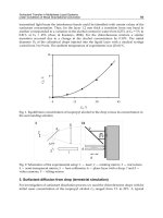
6. Numerical Simulation
In this section, the performance of the MDPSS estimator is compared with the Slepian basis ex-
pansion DPSS approach (Zemen and Mecklenbr
¨
auker; 2005) for a certain radio environment.
The channel model used in the simulations is presented in Section 2.2 and it is simulated using
the AR approach suggested in (Baddour and Beaulieu; 2005). The parameters of the simulated
system are the same as in (Zemen and Mecklenbr
¨

auker; 2005): the carrier frequency is 2 GHz,
the symbol rate used is 48600 1/s, the speed of the user is 102.5 km/h, 10 pilots per data block
are used, and the data block length is M
= 256. The number of DPSS’s used in estimation is
given by
2Mν
D
+ 1. The same number of bases is used for MDPSS, while K = 15 subbands
is used in generation of MDPSS.
50 100 150 200 250
10
−4
10
−3
10
−2
10
−1
10
0
Time Samples in Block
MSE per symbol
MPDSS
DPSS
Fig. 11. Mean square error per symbol for MDPSS (solid) and DPSS (dashed) mobile channel
estimators for the noise-free case.
As an introductory example, consider the estimation accuracy for the WSSUS channel with
a uniform power angle profile (PAS) with central AoA φ
0
= 5 degrees and spread ∆ = 20

degrees. We used 1000 channel realizations and Fig. 11 depicts the results for the considered
channel model. The mean square errors (MSE) for both MDPSS and DPSS estimators have
the highest values at the edges of the data block. However, the MSE for MDPSS estimator is
several orders of magnitude lower than the value for the Slepian basis expansion estimator
based on DPSS.
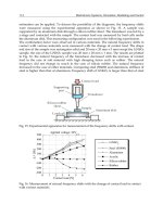
Next, let’s examine the estimation accuracy for the WSSUS channels with uniform PAS, central
AoAs φ
1
= 45 and φ
1
= 75, and spread 0 < ∆ ≤ 2π/3. Furthermore, it is assumed that the
channel is noisy. Figs. 12 and 13 depict the results for SNR
= 10 dB and SNR = 20 dB,
respectively.
The results clearly indicate that the MDPSS frames are a more accurate estimation tool for
the assumed channel model. For the considered angles of arrival and spreading angles, the
MDPSS estimator consistently provided lower MSE in comparison to the Slepian basis expan-
sion estimator based on DPSS. The advantage of the MDPSS stems from the fact that these
bases are able to describe different scattering scenarios.
20 40 60 80 100 120
10
−3
10
−2
10
−1
10
0
Spreading angle (degrees)
MSE

MDPSS for AoA = 45
DPSS for AoA = 45
MDPSS for for AoA = 75
DPSS for for AoA = 75
Fig. 12. Dependence of the MSE on the angular spread ∆ and the mean angle of arrival for
SNR
= 10 dB.
20 40 60 80 100 120
10
−3
10
−2
10
−1
10
0
Spreading angle (degrees)
MSE
MDPSS for AoA = 45
DPSS for AoA = 45
MDPSS for for AoA = 75
DPSS for for AoA = 75
Fig. 13. Dependence of the MSE on the angular spread ∆ and the mean angle of arrival for
SNR
= 20 dB.
7. Conclusions
In this Chapter we have presented a novel approach to modelling MIMO wireless communi-
cation channels. At first, we have argued that in most general settings the distribution of the
in-phase and quadrature components are Gaussian but may have different variance. This was
explained by an insufficient phase randomization by small scattering areas. This model leads

to a non-Rayleigh/non-Rice distribution of magnitude and justifies usage of such generic dis-
tributions as Nakagami or Weibull. It was also shown that additional care should be taken
when modelling specular components in MIMO settings.
Furthermore, based on the assumption that the channel is formed by a collection of relatively
small but non-point scatterers, we have developed a model and a simulation tool to represent
such channels in an orthogonal basis, composed of modulated prolate spheroidal sequences.
Finally MDPSS frames are proposed for estimation of fast fading channels in order to preserve
sparsity of the representation and enhance the estimation accuracy. The members of the frame
WirelessCommunicationsandMultitaperAnalysis:
ApplicationstoChannelModellingandEstimation 43
6. Numerical Simulation
In this section, the performance of the MDPSS estimator is compared with the Slepian basis ex-
pansion DPSS approach (Zemen and Mecklenbr
¨
auker; 2005) for a certain radio environment.
The channel model used in the simulations is presented in Section 2.2 and it is simulated using
the AR approach suggested in (Baddour and Beaulieu; 2005). The parameters of the simulated
system are the same as in (Zemen and Mecklenbr
¨
auker; 2005): the carrier frequency is 2 GHz,
the symbol rate used is 48600 1/s, the speed of the user is 102.5 km/h, 10 pilots per data block
are used, and the data block length is M
= 256. The number of DPSS’s used in estimation is
given by
2Mν
D
+ 1. The same number of bases is used for MDPSS, while K = 15 subbands
is used in generation of MDPSS.
50 100 150 200 250
10

−4
10
−3
10
−2
10
−1
10
0
Time Samples in Block
MSE per symbol
MPDSS
DPSS
Fig. 11. Mean square error per symbol for MDPSS (solid) and DPSS (dashed) mobile channel
estimators for the noise-free case.
As an introductory example, consider the estimation accuracy for the WSSUS channel with
a uniform power angle profile (PAS) with central AoA φ
0
= 5 degrees and spread ∆ = 20
degrees. We used 1000 channel realizations and Fig. 11 depicts the results for the considered
channel model. The mean square errors (MSE) for both MDPSS and DPSS estimators have
the highest values at the edges of the data block. However, the MSE for MDPSS estimator is
several orders of magnitude lower than the value for the Slepian basis expansion estimator
based on DPSS.
Next, let’s examine the estimation accuracy for the WSSUS channels with uniform PAS, central
AoAs φ
1
= 45 and φ
1
= 75, and spread 0 < ∆ ≤ 2π/3. Furthermore, it is assumed that the

channel is noisy. Figs. 12 and 13 depict the results for SNR
= 10 dB and SNR = 20 dB,
respectively.
The results clearly indicate that the MDPSS frames are a more accurate estimation tool for
the assumed channel model. For the considered angles of arrival and spreading angles, the
MDPSS estimator consistently provided lower MSE in comparison to the Slepian basis expan-
sion estimator based on DPSS. The advantage of the MDPSS stems from the fact that these
bases are able to describe different scattering scenarios.
20 40 60 80 100 120
10
−3
10
−2
10
−1
10
0
Spreading angle (degrees)
MSE
MDPSS for AoA = 45
DPSS for AoA = 45
MDPSS for for AoA = 75
DPSS for for AoA = 75
Fig. 12. Dependence of the MSE on the angular spread ∆ and the mean angle of arrival for
SNR
= 10 dB.
20 40 60 80 100 120
10
−3
10

−2
10
−1
10
0
Spreading angle (degrees)
MSE
MDPSS for AoA = 45
DPSS for AoA = 45
MDPSS for for AoA = 75
DPSS for for AoA = 75
Fig. 13. Dependence of the MSE on the angular spread ∆ and the mean angle of arrival for
SNR
= 20 dB.
7. Conclusions
In this Chapter we have presented a novel approach to modelling MIMO wireless communi-
cation channels. At first, we have argued that in most general settings the distribution of the
in-phase and quadrature components are Gaussian but may have different variance. This was
explained by an insufficient phase randomization by small scattering areas. This model leads
to a non-Rayleigh/non-Rice distribution of magnitude and justifies usage of such generic dis-
tributions as Nakagami or Weibull. It was also shown that additional care should be taken
when modelling specular components in MIMO settings.
Furthermore, based on the assumption that the channel is formed by a collection of relatively
small but non-point scatterers, we have developed a model and a simulation tool to represent
such channels in an orthogonal basis, composed of modulated prolate spheroidal sequences.
Finally MDPSS frames are proposed for estimation of fast fading channels in order to preserve
sparsity of the representation and enhance the estimation accuracy. The members of the frame
MobileandWirelessCommunications:Physicallayerdevelopmentandimplementation44
were obtained by modulation and bandwidth variation of DPSS’s in order to reflect various
scattering scenarios. The matching pursuit approach was used to achieve a sparse represen-

tation of the channel. The proposed scheme was tested for various mobile channels, and its
performance was compared with the Slepian basis expansion estimator based on DPSS. The
results showed that the MDPSS method provides more accurate estimation than the DPSS
scheme.
8. References
Alcocer, A., Parra, R. and Kontorovich, V. (2005). An orthogonalization approach for commu-
nication channel modelling, Proc. VTC-2005, Fall.
Alcocer-Ochoa, A., Kontorovitch, V. Y. and Parra-Michel, R. (2006). A MIMO channel simu-
lator applying the universal basis, Proc. of 64th IEEE Vehicular Technology Conference
(VTC-2006), Montreal, QC, Canada.
Algans, A., Pedersen, K. and Mogensen, P. (2002). Experimental analysis of the joint statistical
properties of azimuth spread, delay spread, and shadow fading, IEEE J. Sel. Areas
Commun. 20(3): 523–531.
Almers, P., Bonek, E., Burr, A., Czink, N., Debbah, M., Degli-Esposti, V., Hofstetter, H., Ky
¨
osti,
P., Laurenson, D., Matz, G., Molisch, A. F., Oestges, C. and
¨
Ozcelik, H. (2006). Survey
of channel and radio propagation models for wireless mimo systems.
Andersen, J. and Blaustaein, N. (2003). Multipath Phenomena in Cellular Networks, Artech
House, 2002.
Asplund, H., Glazunov, A., Molisch, A., Pedersen, K. and Steinbauer, M. (2006). The
COST 259 directional channel model Part II: Macrocell, IEEE Trans. Wireless Commun.
5(12): 3434–3450.
Baddour, K. E. and Beaulieu, N. C. (2005). Autoregressive modeling for fading channel simu-
lation, IEEE Transactions on Wireless Communications 4(4): 1650 – 1662.
Barakat, R. (1986). Weak-scatterer generalization of the k-density function with application to
laser scattering in atmospheric turbulence, J. Opt. Soc. Am. A 3(4): 401–409.
Beckmann, P. and Spizzichino, A. (1963). The scattering of electromagnetic waves from rough

surfaces, Pergamon Press, New York, USA.
Bertoni, H. (2000). Radio Propagation For Modern Wireless Systems, Prentice Hall PTR, Upper
Saddle River, NJ.
Blaunstein, N., Toeltsch, M., Laurila, J., Bonek, E., Katz, D., Vainikainen, P., Tsouri, N., Kalliola,
K. and Laitinen, H. (2006). Signal power distribution in the azimuth, elevation and
time delay domains in urban environments for various elevations of base station
antenna, IEEE Trans. Antennas Propag. 54(10): 2902.
Bronez, T. (1992). On the performance advantage of multitaper spectral analysis, IEEE Trans.
Signal Process. 40(12): 2941–2946.
Conover, W. (1998). Practical Nonparametric Statistics, third edn, Wiley, New York.
Fancourt, C. and Principe, J. (2000). On the relationship between the Karhunen-Loeve trans-
form and the prolate spheroidal wave functions, Proc. ICASSP 00, Istambul, Turkey,
pp. 261–264.
Fechtel, S. (1993). A novel approach to modeling and efficient simulation offrequency-selective
fading radio channels, IEEE J. Sel. Areas Commun. 11(3): 422–431.
Fleury, B. (2000). First- and second-order characterization of direction dispersion and space
selectivity in the radio channel, IEEE Trans. Inf. Theory 46(6): 2027–2044.
Jakeman, E. and Tough, R. (1987). Generalized k distribution: a statistical model for weak
scattering, J. Opt. Soc. Am. A 4(9): 1764–1772.
Jeruchim, M. C., Balaban, P. and Shanmugan, K. S. (2000). Simulation of Communication Systems:
Modeling, Methodology and Techniques, New York: Springer.
Kaiserd, T., Bourdoux, A., Boche, H., Fonollosa, J., Andersen, J. and Utschick, W. (2006). Smart
Antennas: State of the Art, Hindawi, NY.
Kirsteins, I., Mehta, S. and Fay, J. (2006). Adaptive separation of unknown narrowband and
broadband time series, Proc. ICASSP 98, Seatlle, WA, USA, pp. 2525–2528.
Klovski, D. (1982). Digital Data Transmission over Radiochannels, Sviaz, Moscow, USSR, (in
Russian).
Kontorovich, V., Primak, S., Alcocer-Ochoa1, A. and Parra-Michel, R. (2008). Mimo channel
orthogonalisations applyinguniversal eigenbasis, Proc. IET Signal processing 2(2): 87–
96.

Kova
ˇ
cevi
´
c, J. and Chabira, A. (2007). Life beyond bases: The advent of the frames (part I),
IEEE Signal Processing Magazine 24(4): 86–104.
Mallat, S. G. (1999). A Wavelet Tour of Signal Processing, second edn, Academic Press, San
Diego.
Mallat, S. G. and Zhang, Z. (1993). Matching pursuits with time-frequency dictionaries, IEEE
Transactions on Signal Processing 41(12): 3397–3415.
Mardia, K. and Jupp, P. (2000). Directional statistics, Wiley, New York.
Molisch, A. F., Asplund, H., Heddergott, R., Steinbauer, M. and Zwick, T. (2006). The COST
259 directional channel model Part I: overview and methodology, IEEE Trans. Wireless
Commun. 5(12): 3421–3433.
Molish, A. (2004). A generic model for MIMO wireless propagation channels in macro- and
microcells, IEEE Trans. Signal Process. 52(1): 61–71.
Papoulis, A. (1991). Probability, Random Variables, and Stochastic Processes, third edn, McGraw-
Hill, Boston, MA.
Patzold, M. (2002). Mobile Fading Channels, John Wiley & Sons, New York.
Percival, D. B. and Walden, A. T. (1993a). Spectral Analysis for Physical Applications: Multitaper
and Conventional Univeriate Techniques, Cambridge University Press, New York.
Percival, D. and Walden, A. (1993b). Spectral Analysis for Physical Applications: Multitaper and
Conventional Univariate Techniques, Cambridge University Press, New York.
Primak, S. and Sejdi
´
c, E. (2008). Application of multitaper analysis to wireless communica-
tions problems, Proc. of First International Symposium on Applied Sciences on Biomedical
and Communication Technologies (ISABEL 2008), Aalborg, Denmark.
Proakis, J. (2001). Digital Communications, fourth edn, McGraw-Hill, New York.
Rao, A. and Hamed, K. (2003). Multi-taper method of analysis of periodicities in hydrologic

data, Journal of Hydrology 279: 125–143.
Rappaport, T. (2002). Wireless Communications: Principles and practice, Prentice Hall, Upper
Saddle River.
Salz, J. and Winters, J. (1994). Effect of fading correlation on adaptive arrays in digital mobile
radio, IEEE Trans. Veh. Technol. 43(4): 1049–1057.
Schreier, P. and Scharf, L. (2003). Second-order analysis of improper complex random vectors
and processes, IEEE Trans. Signal Process. 51(3): 714–725.
SCM Editors (2006). UMTS: Spatial channel model for MIMO simulations, Tech. report 25.996.
Sejdi
´
c, E., Luccini, M., Primak, S., Baddour, K. and Willink, T. (2008). Channel estimation
WirelessCommunicationsandMultitaperAnalysis:
ApplicationstoChannelModellingandEstimation 45
were obtained by modulation and bandwidth variation of DPSS’s in order to reflect various
scattering scenarios. The matching pursuit approach was used to achieve a sparse represen-
tation of the channel. The proposed scheme was tested for various mobile channels, and its
performance was compared with the Slepian basis expansion estimator based on DPSS. The
results showed that the MDPSS method provides more accurate estimation than the DPSS
scheme.
8. References
Alcocer, A., Parra, R. and Kontorovich, V. (2005). An orthogonalization approach for commu-
nication channel modelling, Proc. VTC-2005, Fall.
Alcocer-Ochoa, A., Kontorovitch, V. Y. and Parra-Michel, R. (2006). A MIMO channel simu-
lator applying the universal basis, Proc. of 64th IEEE Vehicular Technology Conference
(VTC-2006), Montreal, QC, Canada.
Algans, A., Pedersen, K. and Mogensen, P. (2002). Experimental analysis of the joint statistical
properties of azimuth spread, delay spread, and shadow fading, IEEE J. Sel. Areas
Commun. 20(3): 523–531.
Almers, P., Bonek, E., Burr, A., Czink, N., Debbah, M., Degli-Esposti, V., Hofstetter, H., Ky
¨

osti,
P., Laurenson, D., Matz, G., Molisch, A. F., Oestges, C. and
¨
Ozcelik, H. (2006). Survey
of channel and radio propagation models for wireless mimo systems.
Andersen, J. and Blaustaein, N. (2003). Multipath Phenomena in Cellular Networks, Artech
House, 2002.
Asplund, H., Glazunov, A., Molisch, A., Pedersen, K. and Steinbauer, M. (2006). The
COST 259 directional channel model Part II: Macrocell, IEEE Trans. Wireless Commun.
5(12): 3434–3450.
Baddour, K. E. and Beaulieu, N. C. (2005). Autoregressive modeling for fading channel simu-
lation, IEEE Transactions on Wireless Communications 4(4): 1650 – 1662.
Barakat, R. (1986). Weak-scatterer generalization of the k-density function with application to
laser scattering in atmospheric turbulence, J. Opt. Soc. Am. A 3(4): 401–409.
Beckmann, P. and Spizzichino, A. (1963). The scattering of electromagnetic waves from rough
surfaces, Pergamon Press, New York, USA.
Bertoni, H. (2000). Radio Propagation For Modern Wireless Systems, Prentice Hall PTR, Upper
Saddle River, NJ.
Blaunstein, N., Toeltsch, M., Laurila, J., Bonek, E., Katz, D., Vainikainen, P., Tsouri, N., Kalliola,
K. and Laitinen, H. (2006). Signal power distribution in the azimuth, elevation and
time delay domains in urban environments for various elevations of base station
antenna, IEEE Trans. Antennas Propag. 54(10): 2902.
Bronez, T. (1992). On the performance advantage of multitaper spectral analysis, IEEE Trans.
Signal Process. 40(12): 2941–2946.
Conover, W. (1998). Practical Nonparametric Statistics, third edn, Wiley, New York.
Fancourt, C. and Principe, J. (2000). On the relationship between the Karhunen-Loeve trans-
form and the prolate spheroidal wave functions, Proc. ICASSP 00, Istambul, Turkey,
pp. 261–264.
Fechtel, S. (1993). A novel approach to modeling and efficient simulation offrequency-selective
fading radio channels, IEEE J. Sel. Areas Commun. 11(3): 422–431.

Fleury, B. (2000). First- and second-order characterization of direction dispersion and space
selectivity in the radio channel, IEEE Trans. Inf. Theory 46(6): 2027–2044.
Jakeman, E. and Tough, R. (1987). Generalized k distribution: a statistical model for weak
scattering, J. Opt. Soc. Am. A 4(9): 1764–1772.
Jeruchim, M. C., Balaban, P. and Shanmugan, K. S. (2000). Simulation of Communication Systems:
Modeling, Methodology and Techniques, New York: Springer.
Kaiserd, T., Bourdoux, A., Boche, H., Fonollosa, J., Andersen, J. and Utschick, W. (2006). Smart
Antennas: State of the Art, Hindawi, NY.
Kirsteins, I., Mehta, S. and Fay, J. (2006). Adaptive separation of unknown narrowband and
broadband time series, Proc. ICASSP 98, Seatlle, WA, USA, pp. 2525–2528.
Klovski, D. (1982). Digital Data Transmission over Radiochannels, Sviaz, Moscow, USSR, (in
Russian).
Kontorovich, V., Primak, S., Alcocer-Ochoa1, A. and Parra-Michel, R. (2008). Mimo channel
orthogonalisations applyinguniversal eigenbasis, Proc. IET Signal processing 2(2): 87–
96.
Kova
ˇ
cevi
´
c, J. and Chabira, A. (2007). Life beyond bases: The advent of the frames (part I),
IEEE Signal Processing Magazine 24(4): 86–104.
Mallat, S. G. (1999). A Wavelet Tour of Signal Processing, second edn, Academic Press, San
Diego.
Mallat, S. G. and Zhang, Z. (1993). Matching pursuits with time-frequency dictionaries, IEEE
Transactions on Signal Processing 41(12): 3397–3415.
Mardia, K. and Jupp, P. (2000). Directional statistics, Wiley, New York.
Molisch, A. F., Asplund, H., Heddergott, R., Steinbauer, M. and Zwick, T. (2006). The COST
259 directional channel model Part I: overview and methodology, IEEE Trans. Wireless
Commun. 5(12): 3421–3433.
Molish, A. (2004). A generic model for MIMO wireless propagation channels in macro- and

microcells, IEEE Trans. Signal Process. 52(1): 61–71.
Papoulis, A. (1991). Probability, Random Variables, and Stochastic Processes, third edn, McGraw-
Hill, Boston, MA.
Patzold, M. (2002). Mobile Fading Channels, John Wiley & Sons, New York.
Percival, D. B. and Walden, A. T. (1993a). Spectral Analysis for Physical Applications: Multitaper
and Conventional Univeriate Techniques, Cambridge University Press, New York.
Percival, D. and Walden, A. (1993b). Spectral Analysis for Physical Applications: Multitaper and
Conventional Univariate Techniques, Cambridge University Press, New York.
Primak, S. and Sejdi
´
c, E. (2008). Application of multitaper analysis to wireless communica-
tions problems, Proc. of First International Symposium on Applied Sciences on Biomedical
and Communication Technologies (ISABEL 2008), Aalborg, Denmark.
Proakis, J. (2001). Digital Communications, fourth edn, McGraw-Hill, New York.
Rao, A. and Hamed, K. (2003). Multi-taper method of analysis of periodicities in hydrologic
data, Journal of Hydrology 279: 125–143.
Rappaport, T. (2002). Wireless Communications: Principles and practice, Prentice Hall, Upper
Saddle River.
Salz, J. and Winters, J. (1994). Effect of fading correlation on adaptive arrays in digital mobile
radio, IEEE Trans. Veh. Technol. 43(4): 1049–1057.
Schreier, P. and Scharf, L. (2003). Second-order analysis of improper complex random vectors
and processes, IEEE Trans. Signal Process. 51(3): 714–725.
SCM Editors (2006). UMTS: Spatial channel model for MIMO simulations, Tech. report 25.996.
Sejdi
´
c, E., Luccini, M., Primak, S., Baddour, K. and Willink, T. (2008). Channel estimation
MobileandWirelessCommunications:Physicallayerdevelopmentandimplementation46
using DPSS based frames, Proc. of IEEE International Conf. on Acoustics, Speech, and
Signal Processing (ICASSP 2008), Las Vegas, USA, pp. 2849–2852.
Sen, I. and Matolak, D. (2008). Vehiclevehicle channel models for the 5-GHz band, IEEE Trans.

Intell. Transp. Syst. 9(26): 235–245.
Simon, M. and Alouini, M S. (2000). Digital Communication over Fading Channels:A Unified
Approach to Performance Analysis, John Wiley & Sons, New York.
Slepian, D. (1978). Prolate spheroidal wave functions, Fourier analysis, and uncertainty. V-The
discrete case, Bell System Technical Journal 57: 1371–1430.
Stoica, P. and Sundin, T. (1999). On nonparametric spectral estimation, Journal of Circuits,
Systems, and Signal Processing 18(2): 169–181.
Thomson, D. (1998). Multiple-window spectrum estimates for non-stationary data, Proc. of
Ninth IEEE SP Workshop on Statistical Signal and Array Processing, 1998, pp. 344–347.
Thomson, D. (2000). Multitaper Analysis of Nonstationary and Nonlinear Time Series Data,
Nonlinear and Nonstationary Signal Processing .
Thomson, D. J. (1982). Spectrum estimation and harmonic analysis, Proceedings of the IEEE
70(9): 1055–1096.
van Trees, H. (2001). Detection, Estimation, and Moduclation Theory: Part I, first edn, John Wiley
& Sons, New York.
van Trees, H. (2002). Detection, Estimation and Modulation Theory: Optimal Array Processing, first
edn, Wiley-Interscience, New York.
Xiao, H., Burr, A. and White, G. (2005). Simulation of time-selective environment by 3GPP
spatial channel model and analysis on the performance evaluation by the CMD met-
ric, Proc. International Wireless Summit (IWS 05), Aalborg, Denmark, pp. 446–450.
Yip, K. and Ng, T. (1997). Karhunen-Loeve expansion of the WSSUS channel output and its
application to efficient simulation, IEEE J. Sel. Areas Commun. 15(4): 640–646.
Zemen, T., Hofstetter, H. and Steinbck, G. (2005). Slepian subspace projection in time and
frequency for time-variant channel estimation, 14th IST Mobile and Wireless Summit,
Dresden, Germany.
Zemen, T. and Mecklenbr
¨
auker, C. F. (2005). Time-variant channel estimation using discrete
prolate spheroidal sequences, IEEE Transactions on Signal Processing 53(9): 3597–3607.
Zemen, T., Mecklenbr

¨
auker, C. F. and Fleury, B. (2006). Time-variant channel prediction us-
ing time-concentrated and band-limited sequences, Proc. of 2006 IEEE International
Conference on Communications (ICC ’06), Vol. 12, Istanbul, Turkey, pp. 5660–5665.
HighAltitudePlatformsforWirelessMobileCommunicationApplications 47
HighAltitudePlatformsforWirelessMobileCommunicationApplications
ZheYangandAbbasMohammed
X

High Altitude Platforms for Wireless Mobile
Communication Applications

Zhe Yang and Abbas Mohammed
Blekinge Institute of Technology
Sweden

1. Introduction
The wireless communications field has experienced an extraordinary development during
the past two decades or so. New wireless technologies give people more convenience and
freedom to connect to different communication networks. It is thought that the demand for
the capacity increases significantly when the next generation of multimedia applications are
combined with future wireless communication systems.

Wireless communication services are typically provided by terrestrial and satellite systems.
The successful and rapid deployment of both wireless networks has illustrated the growing
demand for broadband mobile communications. These networks are featured with high
data rates, reconfigurable support, dynamic time and space coverage demand with
considerable cost. Terrestrial links are widely used to provide services in areas with complex
propagation conditions and in mobile applications. Satellite links are usually used to
provide high speed connections where terrestrial links are not available. In parallel with

these well established networks, a new alternative using aerial high altitude platforms
(HAPs) has emerged and attracted international attentions (Mohammed et al., 2008).

Communications platforms situated at high altitudes can be dated to the last century. In
1960 a giant balloon was launched in USA. It reflected broadcasts from the Bell laboratories
facility at Crawford Hill and bounced the signals to long distance telephone call users. This
balloon can be regarded as an ancestor of HAPs. Traditional applications of airships have
been restricted in entertainment purposes, meteorological usage, and environment
surveillance due to safety reasons. However, in the past few years, technological
advancements in communications from airships has given a promising future in this area
(Karapantazis & Pavlidou, 2005).

HAPs are airships or planes, operating in the stratosphere, at altitudes of typically 17-22 km
(around 75,000 ft) (Collela et al., 2000; Hult et al., 2008b; Mohammed et al., 2008; Yang &
Mohammed, 2008b). At this altitude (which is well above commercial aircraft height), they
can support payloads to deliver a range of services: principally communications and remote
sensing. A HAP can provide the best features of both terrestrial masts (which may be subject
3
MobileandWirelessCommunications:Physicallayerdevelopmentandimplementation48

to planning restrictions and/or related environmental/health constraints) and satellite
systems (which are usually highly expensive) (Cost 297, 2005; Mohammed et al., 2008). This
makes HAP a viable competitor/complement to conventional terrestrial infrastructures and
satellite systems. Thus HAPs are regarded as a future candidate for next generation systems,
either as a stand-alone system or integrated with other satellite or terrestrial systems.

HAPs as a new solution for delivering wireless broadband, have been recently proposed for
the provision of fixed, mobile services and application as shown in Fig. 1 (Grace et al., 2001b;
Yang & Mohammed, 2008a). HAPs can act as base-stations or relay nodes, which may be
effectively regarded as a very tall antenna mast or a very Low-Earth-Orbit (LEO) satellite

(Thornton et al., 2001). This modern communication solution has advantages of both
terrestrial and satellite communications (Djuknic et al., 1997; Steele, 1992). It is a good
technique for serving the increasing demand of Broadband Wireless Access (BWA) by using
higher frequency allocations especially in mm-wavelength and high-speed data capacity.
HAPs are also proposed to provide other communication services, i.e. the 3
rd
generation
(3G) services. The International Telecommunication Union (ITU) gave licensed a frequency
band around 2 GHz for IMT-2000 service (Grace et al., 2001a). An optical inter-platform link
can be established between platforms to expand a network in the altitude to cover a large
area. A broadband access link between the platform and user on the ground can be
established to support different applications. Fixed, mobile and portable user terminals can
be supported by the system. With assistance of terrestrial networks, HAPs can also provide
the telecommunication services or the backbone for terrestrial networks in remote areas.

Fig. 1. HAP system deployed at 17~22 km above the ground

The full chapter is organized as follows: in section 1, we give an introduction to the HAP
concept in wireless communications. In section 2, an overview of communication
applications from HAPs, frequency allocations, well-known HAP research activities and

trials are given. In section 3, main characteristics of HAP system are summarized and
scenarios of HAP deployment are discussed. Finally, conclusions and future research are
given in section 4.
2. Applications, Research and Trials of HAP Systems
2.1 Applications and frequency allocations of HAP System
HAPs have been proposed to deliver modern broadband services, i.e. high-speed internet,
High-Definition Television (HDTV), Local Multi-Point Distribution (LMDS), Multi-Channel
Multimedia Distribution Service (MMDS), and Wireless Interoperability for Microwave
Access (WiMAX). All these services require wide bandwidth and high capacity. Generally

these applications can be thought to equip base stations onboard, and based on well
established terrestrial system design experience, but they are facing new challenges, e.g. cell
structures, handover controls and dynamic channel assignment.

BWA services operate in the higher frequency bands, i.e. the mm-wave bands at several
GHz, to provide the required radio frequency bandwidth allocation. The frequency bands
allocated for LMDS in most countries in the world are around 30 GHz. ITU has assigned
frequency bands of 47-48 GHz to HAPs worldwide. The 28-31 GHz bands have also
assigned to HAP in some regions.

 On the ITU 1997 World Radio communication Conference (WRC-97), the ITU
passed the RESOLUTION 122 to use the bands 47.2-47.5 GHz and 47.9-48.2 GHz
for HAPs to provide the Fixed Service (FS) (ITU-R, 2003). WRC-2000 adopted the
revision of RESOLUTION 122 to allow HAPs utilizing the bands 18-32 GHz, 27.5-
28.35 GHz and 31-31.3 GHz in interested countries on non-interference and non-
protection basis, which extended the previous RESOLUTION 122 (ITU-R, 2003). At
the recent WRC-03 in ITU 2003, ITU gave the temporary RESOLUTION 145
[COM5/17] for potential using of the bands 27.5-28.35 GHz and HAPs in the FS
(ITU-R, 2003).

HAPs may be one of the most important infrastructures for International Mobile
Telecommunications (IMT-2000) 3G service, since HAPs can offer new means to provide
IMT-2000 service with minimal network infrastructure. IMT-2000 standard has included
provision for base-station deployment from HAPs and still needs further study before the
deployment from HAPs in the areas of cell planning and antenna development. Employing
access techniques such as Code Division Multiple Access (CDMA), Wideband-CDMA (W-
CDMA) based IMT-2000 and CDMA based universal mobile telecommunications system
(UMTS) from HAPs to provide 3G communications have been examined. (Foo et al., 2002;
Hult et al., 2008a)

 RESOLUTION 221 was adopted by WRC-00 in ITU 2000 to approve HAPs
providing IMT-2000 in the bands 1885-1980 MHz, 2010-2025 MHz and 2110-2170
MHz in with explicit region restrictions (ITU-R, 2003).
HighAltitudePlatformsforWirelessMobileCommunicationApplications 49

to planning restrictions and/or related environmental/health constraints) and satellite
systems (which are usually highly expensive) (Cost 297, 2005; Mohammed et al., 2008). This
makes HAP a viable competitor/complement to conventional terrestrial infrastructures and
satellite systems. Thus HAPs are regarded as a future candidate for next generation systems,
either as a stand-alone system or integrated with other satellite or terrestrial systems.

HAPs as a new solution for delivering wireless broadband, have been recently proposed for
the provision of fixed, mobile services and application as shown in Fig. 1 (Grace et al., 2001b;
Yang & Mohammed, 2008a). HAPs can act as base-stations or relay nodes, which may be
effectively regarded as a very tall antenna mast or a very Low-Earth-Orbit (LEO) satellite
(Thornton et al., 2001). This modern communication solution has advantages of both
terrestrial and satellite communications (Djuknic et al., 1997; Steele, 1992). It is a good
technique for serving the increasing demand of Broadband Wireless Access (BWA) by using
higher frequency allocations especially in mm-wavelength and high-speed data capacity.
HAPs are also proposed to provide other communication services, i.e. the 3
rd
generation
(3G) services. The International Telecommunication Union (ITU) gave licensed a frequency
band around 2 GHz for IMT-2000 service (Grace et al., 2001a). An optical inter-platform link
can be established between platforms to expand a network in the altitude to cover a large
area. A broadband access link between the platform and user on the ground can be
established to support different applications. Fixed, mobile and portable user terminals can
be supported by the system. With assistance of terrestrial networks, HAPs can also provide
the telecommunication services or the backbone for terrestrial networks in remote areas.

Fig. 1. HAP system deployed at 17~22 km above the ground

The full chapter is organized as follows: in section 1, we give an introduction to the HAP
concept in wireless communications. In section 2, an overview of communication
applications from HAPs, frequency allocations, well-known HAP research activities and

trials are given. In section 3, main characteristics of HAP system are summarized and
scenarios of HAP deployment are discussed. Finally, conclusions and future research are
given in section 4.
2. Applications, Research and Trials of HAP Systems
2.1 Applications and frequency allocations of HAP System
HAPs have been proposed to deliver modern broadband services, i.e. high-speed internet,
High-Definition Television (HDTV), Local Multi-Point Distribution (LMDS), Multi-Channel
Multimedia Distribution Service (MMDS), and Wireless Interoperability for Microwave
Access (WiMAX). All these services require wide bandwidth and high capacity. Generally
these applications can be thought to equip base stations onboard, and based on well
established terrestrial system design experience, but they are facing new challenges, e.g. cell
structures, handover controls and dynamic channel assignment.

BWA services operate in the higher frequency bands, i.e. the mm-wave bands at several
GHz, to provide the required radio frequency bandwidth allocation. The frequency bands
allocated for LMDS in most countries in the world are around 30 GHz. ITU has assigned
frequency bands of 47-48 GHz to HAPs worldwide. The 28-31 GHz bands have also
assigned to HAP in some regions.

 On the ITU 1997 World Radio communication Conference (WRC-97), the ITU
passed the RESOLUTION 122 to use the bands 47.2-47.5 GHz and 47.9-48.2 GHz
for HAPs to provide the Fixed Service (FS) (ITU-R, 2003). WRC-2000 adopted the
revision of RESOLUTION 122 to allow HAPs utilizing the bands 18-32 GHz, 27.5-
28.35 GHz and 31-31.3 GHz in interested countries on non-interference and non-

protection basis, which extended the previous RESOLUTION 122 (ITU-R, 2003). At
the recent WRC-03 in ITU 2003, ITU gave the temporary RESOLUTION 145
[COM5/17] for potential using of the bands 27.5-28.35 GHz and HAPs in the FS
(ITU-R, 2003).

HAPs may be one of the most important infrastructures for International Mobile
Telecommunications (IMT-2000) 3G service, since HAPs can offer new means to provide
IMT-2000 service with minimal network infrastructure. IMT-2000 standard has included
provision for base-station deployment from HAPs and still needs further study before the
deployment from HAPs in the areas of cell planning and antenna development. Employing
access techniques such as Code Division Multiple Access (CDMA), Wideband-CDMA (W-
CDMA) based IMT-2000 and CDMA based universal mobile telecommunications system
(UMTS) from HAPs to provide 3G communications have been examined. (Foo et al., 2002;
Hult et al., 2008a)

 RESOLUTION 221 was adopted by WRC-00 in ITU 2000 to approve HAPs
providing IMT-2000 in the bands 1885-1980 MHz, 2010-2025 MHz and 2110-2170
MHz in with explicit region restrictions (ITU-R, 2003).
MobileandWirelessCommunications:Physicallayerdevelopmentandimplementation50

 RESOLUTION 734, which proposed HAPs to operate in the frequency range of 3-
18 GHz, was adopted by WRC-2000 to allow these studies. It is noted that the range
of 10.6 to 18 GHz range was not allocated to match the RESOLUTION 734.

2.2 HAP research and trails in the World
Many countries and organizations have made significant efforts in the research of HAPs
system and its applications. Some well-known projects are listed below:
 The US Lockheed Martin compnay has won a contract from US Defense Advanced
Research Projects Agency (DARPA) and the US Air Force (USAF) to build a high-
altitude airship demonstrator featuring radar technology powerful enough to

detect a car hidden under a canopy of trees from a distance of more than 300 km.
Lockheed's Skunk Works division will build and fly a demonstrator aircraft with a
scaled-down sensor system in fiscal year 2013 (Flightglobal, 2009).
 Since 2005 the EU Cost 297 action has been established in order to increase
knowledge and understanding of the use of HAPs for delivery of communications
and other services. It is now the largest gathering of research community with
interest in HAPs and related technologies (Cost 297, 2005; Mohammed et al., 2008).
 CAPANINA of the European Union (EU) - The primary aim of CAPANINA is to
provide technology that will deliver low-cost broadband communications services
to small office and home users at data rates up to 120 Mbit/s. Users in rural areas
will benefit from the unique wide-area, high-capacity coverage provided by HAPs.
Trials of the technology are planned during the course of the project. Involving 13
global partners, this project is developing wireless and optical broadband
technologies that will be used on HAPs (Grace et al., 2005).
 SkyNet project in Japan - A Japanese project lanuched at the beginning in 1998 to
develop a HAP and studying equipments for delivery of broadband and 3G
communications. This aim of the project was the development of the on-board
communication equipment, wireless network protocols and platforms (Hong et al.,
2005)
 European Space Agency (ESA) - has completed research of broadband delivery
from HAPs. Within this study a complete system engineering process was
performed for aerostatic stratospheric platforms. It has shown the overall system
concept of a stratospheric platform and a possible way for its implementation (ESA,
2005).
 Lindstrand Balloons Ltd. (LBL) - The team in this company has been building
lighter-than-air vehicles for almost 21 years. They have a series of balloon
developments including Stratospheric Platforms, Sky Station, Ultra Long Distance
Balloon (ULDB-NASA) (Lindstrand Balloons Ltd, 2005).
 HALE - The application of High-Altitude Long Endurance (HALE) platforms in
emergency preparedness and disaster management and mitigation is led by the

directorate of research and development in the office of critical infrastructure
protection and emergency preparedness in Canada. The objective of this project
has been to assess the potential application of HALE-based remote sensing
technologies to disaster management and mitigation. HALE systems use advanced
aircraft or balloon technologies to provide mobile, usually uninhabited, platforms
operating at altitudes in excess of 50,000 feet (15,000 m) (OCIPEP, 2000).

 An US compnay Sanswire Technologies Inc. (Fort Lauderdale, USA) and Angel
Technologies (St. Louis, USA) carried out a series of research and demonstrations
for HAP practical applications. The flight took place at the Sanswire facility in
Palmdale, California, on Nov. 15, 2005. These successful demonstrations represent
mature steps in the evolution of Sanswire's overall high altitude airship program.
 Engineers from Japan have demonstrated that HAPs can be used to provide HDTV
services and IMT-2000 WCDMA services successfully.

A few HAP trails have been carried out in the EU CAPANINA project to demonstrate its
capabilities and applications (CAPANINA, 2004).
 In 2004, the first trial was in Pershore, UK. The trial consisted of a set of several
tests based on a 300 m altitude tethered aerostat. Though the aerostat was not
situated at the expected altitude it have many tasks of demonstrations and
assessments, e.g. BFWA up to 120 Mbps to a fixed user using 28 GHz band, end-to-
end network connectivity, high speed Internet, Video On Demand (VoD) service,
using a similar platform-user architecture as that of a HAP.
 In October 2005, the second trial was conducted in Sweden. A 12,000 cubic meter
balloon, flying at an altitude of around 24 km for nine hours, was launched. It
conducted the RF and optical trials. Via Wi-Fi the radio equipment has supported
date rates of 11 Mbps at distances ranging up to 60 km. This trial is a critical step to
realize the ultimate term aim of CAPANINA to provide the 120 Mpbs data rate.
3. HAP Communication System and Deployment
3.1 Advantages of HAP system

HAPs are regarded to have several unique characteristics compared with terrestrial and
satellite systems, and are ideal complement or alternative solutions when deploying next
generation communication system requiring high capacity. Typical characteristics of these
three systems are shown in Table 1.
Subject HAPs Terrestrial Satellite
Cell radius 3~7 km 0.1~2 km 50 km for LEO
BS Coverage area
radius
Typical 30 km
ITU has suggested 150 km
5 km A few hundred km
for LEO
Elevation angles High Low High
Propagation delay Low Low Noticeable
Propagation
Characteristic
Nearly Fress Space Path
Loss (FSPL)
Well established,
typically Non FPSL
FPSL with rain
BS power supply Fuel (ideally solar) Electricity Solar
BS maintenance Less complexity in terms of
coverage area
Complex if multiple
BSs needed to update
Impossible
BS cost No specific number but
supposed to be economical
in terms of coverage area

Well established
market, cost
depending on the
companies
5 billion for Iridium,
Very expensive
Operational Cost Medium (mainly airship
maintenance)
Medium ~ High in
terms of the number of
BSs
High
Deployment
complexity
Low (especially in remote
and high density
population area)
Medium (more
complex to deploy in
the city area)
High
Table 1. System characteristics of HAP, terrestrial and satellite systems.