RECENT ADVANCES IN ROBUST CONTROL – NOVEL APPROACHES AND DESIGN METHODSE Part 2 potx

Robust Stabilization by Additional Equilibrium

19


Fig. 21. Behavior of output of the submarine depth control system at various a
23
.



Fig. 22. Behavior of output of the submarine depth control system at various a
32
.


Fig. 23. Behavior of output of the submarine depth control system at various a
33
.

Recent Advances in Robust Control – Novel Approaches and Design Methods

20
4. Conclusion
Adding the equilibria that attracts the motion of the system and makes it stable can give
many advantages. The main of them is that the safe ranges of parameters are widened
significantly because the designed system stay stable within unbounded ranges of
perturbation of parameters even the sign of them changes. The behaviors of designed
control systems obtained by MATLAB simulation such that control of linear and nonlinear
dynamic plants confirm the efficiency of the offered method. For further research and

investigation many perspective tasks can occur such that synthesis of control systems with
special requirements, design of optimal control and many others.
5. Acknowledgment
I am heartily thankful to my supervisor, Beisenbi Mamirbek, whose encouragement,
guidance and support from the initial to the final level enabled me to develop an
understanding of the subject. I am very thankful for advises, help, and many offered
opportunities to famous expert of nonlinear dynamics and chaos Steven H. Strogatz, famous
expert of control systems Marc Campbell, and Andy Ruina Lab team.
Lastly, I offer my regards and blessings to all of those who supported me in any respect
during the completion of the project.
6. References
Beisenbi, M; Ten, V. (2002). An approach to the increase of a potential of robust stability of
control systems, Theses of the reports of VII International seminar «Stability and
fluctuations of nonlinear control systems» pp. 122-123, Moscow, Institute of problems
of control of Russian Academy of Sciences, Moscow, Russia
Ten, V. (2009). Approach to design of Nonlinear Robust Control in a Class of Structurally
Stable Functions, Available from
V.I. Arnold, A.A. Davydov, V.A. Vassiliev and V.M. Zakalyukin (2006). Mathematical Models
of Catastrophes. Control of Catastrohic Processes. EOLSS Publishers, Oxford, UK
Dorf, Richard C; Bishop, H. (2008). Modern Control Systems, 11/E. Prentice Hall, New Jersey,
USA
Khalil, Hassan K. (2002). Nonlinear systems. Prentice Hall, New Jersey, USA
Gu, D W ; Petkov, P.Hr. ; Konstantinov, M.M. (2005). Robust control design with Matlab.
Springer-Verlag, London, UK
Poston, T.; Stewart, Ian. (1998). Catastrophe: Theory and Its Applications. Dover, New York,
USA
0
Robust Control of Nonlinear Time-Delay Systems
via Takagi-Sugeno Fuzzy Models
Hamdi Gassara

1,2
, Ahmed El Hajjaji
1
and Mohamed Chaabane
3
1
Modeling, Information, and Systems Laboratory, University of Picardie
Jules Verne, Amiens 80000,
2
Department of Electrical Engineering, Unit of Control of Industrial Process,
National School of Engineering, University of Sfax, Sfax 3038
3
Automatic control at National School of Engineers of Sfax (ENIS)
1
France
2,3
Tunisia
1. Introduction
Robust control theory is an interdisciplinary branch of engineering and applied mathematics
literature. Since its introduction in 1980’s, it has grown to become a major scientific domain.
For example, it gained a foothold in Economics in the late 1990 and has seen increasing
numbers of Economic applications in the past few years. This theory aims to design
a controller which guarantees closed-loop stability and performances of systems in the
presence of system uncertainty. In practice, the uncertainty can include modelling errors,
parametric variations and external disturbance. Many results have been presented for
robust control of linear systems. However, most real physical systems are nonlinear in
nature and usually subject to uncertainties. In this case, the linear dynamic systems are not
powerful to describe these practical systems. So, it is important to design robust control of
nonlinear models. In this context, different techniques have been proposed in the literature
(Input-Output linearization technique, backstepping technique, Variable Structure Control

(VSC) technique, ).
These two last decades, fuzzy model control has been extensively studied; see
(Zhang & Heng, 2002)-(Chadli & ElHajjaji, 2006)-(Kim & Lee, 2000)-(Boukas & ElHajjaji, 2006)
and the references therein because T-S fuzzy model can provide an effective representation
of complex nonlinear systems. On the other hand, time-delay are often occurs in various
practical control systems, such as transportation systems, communication systems, chemical
processing systems, environmental systems and power systems. It is well known that the
existence of delays may deteriorate the performances of the system and can be a source of
instability. As a consequence, the T-S fuzzy model has been extended to deal with nonlinear
systems with time-delay. The existing results of stability and stabilization criteria for this
class of T-S fuzzy systems can be classified into two types: delay-independent, which are
applicable to delay of arbitrary size (Cao & Frank, 2000)-(Park et al., 2003)-(Chen & Liu,
2005b), and delay-dependent, which include information on the size of delays, (Li et al.,
2004) - (Chen & Liu, 2005a). It is generally recognized that delay-dependent results are
usually less conservative than delay-independent ones, especially when the size of delay
2
2 Will-be-set-by-IN-TECH
is small. We notice that all the results of analysis and synthesis delay-dependent methods
cited previously are based on a single LKF that bring conservativeness in establishing
the stability and stabilization test. Moreover, the model transformation, the conservative
inequalities and the so-called Moon’s inequality (Moon et al., 2001) for bounding cross
terms used in these methods also bring conservativeness. Recently, in order to reduce
conservatism, the weighting matrix technique was proposed originally by He and al. in
(He et al., 2004)-(He et al., 2007). These works studied the stability of linear systems with
time-varying delay. More recently, Huai-Ning et al. (Wu & Li, 2007) treated the problem
of stabilization via PDC (Prallel Distributed Compensation) control by employing a fuzzy
LKF combining the introduction of free weighting matrices which improves existing ones in
(Li et al., 2004) - (Chen & Liu, 2005a) without imposing any bounding techniques on some
cross product terms. In general, the disadvantage of this new approach (Wu & Li, 2007) lies in
that the delay-dependent stabilization conditions presented involve three tuning parameters.

Chen et al. in (Chen et al., 2007) and in (Chen & Liu, 2005a) have proposed delay-dependent
stabilization conditions of uncertain T-S fuzzy systems. The inconvenience in these works is
that the time-delay must be constant. The designing of observer-based fuzzy control and the
introduction of performance with guaranteed cost for T-S with input delay have discussed in
(Chen, Lin, Liu & Tong, 2008) and (Chen, Liu, Tang & Lin, 2008), respectively.
In this chapter, we study the asymptotic stabilization of uncertain T-S fuzzy systems with
time-varying delay. We focus on the delay-dependent stabilization synthesis based on the
PDC scheme (Wang et al., 1996). Different from the methods currently found in the literature
(Wu & Li, 2007)-(Chen et al., 2007), our method does not need any transformation in the
LKF, and thus, avoids the restriction resulting from them. Our new approach improves
the results in (Li et al., 2004)-(Guan & Chen, 2004)-(Chen & Liu, 2005a)-(Wu & Li, 2007) for
three great main aspects. The first one concerns the reduction of conservatism. The second
one, the reduction of the number of LMI conditions, which reduce computational efforts.
The third one, the delay-dependent stabilization conditions presented involve a single fixed
parameter. This new approach also improves the work of B. Chen et al. in (Chen et al., 2007)
by establishing new delay-dependent stabilization conditions of uncertain T-S fuzzy systems
with time varying delay. The rest of this chapter is organized as follows. In section 2, we
give the description of uncertain T-S fuzzy model with time varying delay. We also present
the fuzzy control design law based on PDC structure. New delay dependent stabilization
conditions are established in section 3. In section 4, numerical examples are given to
demonstrate the effectiveness and the benefits of the proposed method. Some conclusions are
drawn in section 5.
Notation:

n
denotes the n-dimensional Euclidiean space. The notation P > 0 means that P is
symmetric and positive definite. W
+ W
T
is denoted as W +(∗) for simplicity. In symmetric

bloc matrices, we use
∗ as an ellipsis for terms that are induced by symmetry.
2. Problem formulation
Consider a nonlinear system with state-delay which could be represented by a T-S fuzzy
time-delay model described by
Plant Rule i
(i = 1, 2,···, r):If θ
1
is μ
i1
and ··· and θ
p
is μ
ip
THEN
˙
x
(t)=(A
i
+ ΔA
i
)x(t)+(A
τi
+ ΔA
τi
)x(t −τ(t)) + (B
i
+ ΔB
i
)u(t)

x(t)=ψ(t), t ∈ [−τ,0],
(1)
22
Recent Advances in Robust Control – Novel Approaches and Design Methods
Robust Control of Nonlinear Time-Delay Systems via Takagi-Sugeno Fuzzy Models 3
where θ
j
(x(t)) and μ
ij
(i = 1, ···, r, j = 1, ···, p) are respectively the premise variables and
the fuzzy sets; ψ
(t) is the initial conditions; x(t) ∈
n
is the state; u(t) ∈
m
is the control
input; r is the number of IF-THEN rules; the time delay, τ
(t), is a time-varying continuous
function that satisfies
0
≤ τ(t ) ≤ τ,
˙
τ(t) ≤ β (2)
The parametric uncertainties ΔA
i
, ΔA
τi
, ΔB
i
are time-varying matrices that are defined as

follows
ΔA
i
= M
Ai
F
i
(t)E
Ai
,; ΔA
τi
= M
Aτi
F
i
(t)E
Aτi
,; ΔB
i
= M
Bi
F
i
(t)E
Bi
(3)
where M
Ai
, M
Aτi

, M
Bi
, E
Ai
, E
Aτi
, E
Bi
are known constant matrices and F
i
(t) is an unknown
matrix function with the property
F
i
(t)
T
F
i
(t) ≤ I (4)
Let
¯
A
i
= A
i
+ ΔA
i
;
¯
A

τi
= A
τi
+ ΔA
τi
;
¯
B
i
= B
i
+ ΔB
i
By using the common used center-average defuzzifier, product inference and singleton
fuzzifier, the T-S fuzzy systems can be inferred as
˙
x
(t)=
r
∑
i=1
h
i
(θ(x(t)))[
¯
A
i
x(t)+
¯
A

τi
x(t − τ(t)) +
¯
B
i
u(t)] (5)
where θ
(x(t)) = [θ
1
(x(t)), ···,θ
p
(x(t))] and ν
i
(θ(x(t))) : 
p
→ [0, 1], i = 1, ···,r,isthe
membership function of the system with respect to the ith plan rule. Denote h
i
(θ(x(t))) =
ν
i
(θ(x(t)))/
∑
r
i
=1
ν
i
(θ(x(t))). It is obvious that
h

i
(θ(x(t))) ≥ 0and
∑
r
i
=1
h
i
(θ(x(t))) = 1
the design of state feedback stabilizing fuzzy controllers for fuzzy system (5) is based on the
Parallel Distributed Compensation.
Controller Rule i
(i = 1, 2, ···, r):If θ
1
is μ
i1
and ··· and θ
p
is μ
ip
THEN
u
(t)=K
i
x(t) (6)
The overall state feedback control law is represented by
u
(t)=
r
∑

i=1
h
i
(θ(x(t)))K
i
x(t) (7)
In the sequel, for brevity we use h
i
to denote h
i
(θ(x(t))). Combining (5) with (7), the
closed-loop fuzzy system can be expressed as follows
˙
x
(t)=
r
∑
i=1
r
∑
j=1
h
i
h
j
[

A
ij
x(t)+

¯
A
τi
x(t −τ(t))] (8)
with

A
ij
=
¯
A
i
+
¯
B
i
K
j
In order to obtain the main results in this chapter, the following lemmas are needed
23
Robust Control of Nonlinear Time-Delay Systems via Takagi-Sugeno Fuzzy Models
4 Will-be-set-by-IN-TECH
Lemma 1. (Xie & DeSouza, 1992)-(Oudghiri et al., 2007) (Guerra et al., 2006) Considering Π < 0 a
matrix X and a scalar λ, the following holds
X
T
ΠX ≤−2λX −λ
2
Π
−1

(9)
Lemma 2. (Wang et al., 1992) Given matrices M, E, F
(t) with compatible dimensions and F(t)
satisfying F(t)
T
F(t) ≤ I.
Then, the following inequalities hold for any 
> 0
MF
(t)E + E
T
F(t)
T
M
T
≤ MM
T
+ 
−1
E
T
E (10)
3. Main results
3.1 Time-delay dependent stability conditions
First, we derive the stability condition for unforced system (5), that is
˙
x
(t)=
r
∑

i=1
h
i
[
¯
A
i
x(t)+
¯
A
τi
x(t −τ(t))] (11)
Theorem 1. System (11) is asymptotically stable, if there exist some matrices P
> 0, S > 0, Z > 0, Y
and T satisfying the following LMIs for i
= 1, 2, , r
⎡
⎢
⎢
⎢
⎢
⎢
⎢
⎣
ϕ
i
+ 
Ai
E
T

Ai
E
Ai
PA
τi
−Y + T
T
A
T
i
Z −YPM
Ai
PM
Aτi
∗−(1 − β)S − T −T
T
+ 
Aτi
E
T
τi
E
τi
A
T
τi
Z −T 0
∗∗−
1
τ

Z 0 ZM
Ai
ZM
Aτi
∗∗∗−
1
τ
Z 0
∗∗∗∗−
Ai
I 0
∗∗∗∗∗−
Aτi
I
⎤
⎥
⎥
⎥
⎥
⎥
⎥
⎦
< 0 (12)
where ϕ
i
= PA
i
+ A
T
i

P + S + Y + Y
T
.
Proof 1. Choose the LKF as
V
(x(t)) = x(t)
T
Px(t)+

t
t
−τ(t)
x(α)
T
Sx(α) dα +

0
−τ

t
t
+σ
˙
x
(α)
T
Z
˙
x(α)dαdσ (13)
the time derivative of this LKF (13) along the trajectory of system (11) is computed as

˙
V
(x(t)) = 2x(t)
T
P
˙
x(t)+x(t)
T
Sx(t) −(1 −
˙
τ
(t)) x(t − τ(t))
T
Sx(t − τ(t))
+
τ
˙
x(t)
T
Z
˙
x(t) −

t
t
−τ
˙
x
(s)
T

Z
˙
x(s)ds
(14)
Taking into account the Newton-Leibniz formula
x
(t − τ(t)) = x(t) −

t
t
−τ(t)
˙
x
(s)ds (15)
We obtain equation (16)
24
Recent Advances in Robust Control – Novel Approaches and Design Methods
Robust Control of Nonlinear Time-Delay Systems via Takagi-Sugeno Fuzzy Models 5
˙
V
(x(t)) =
r
∑
i=1
h
i
[2x(t)
T
P
¯

A
i
x(t)+2x(t)
T
P
¯
A
τi
x(t −τ(t))]
+
x(t)
T
Sx(t) −(1 − β)x(t − τ(t))
T
Sx(t −τ(t))
+
τ
˙
x(t)
T
Z
˙
x(t) −

t
t
−τ
˙
x
(s)

T
Z
˙
x(s)ds
+2[x(t)
T
Y + x(t − τ(t))
T
T] × [x (t) − x(t − τ(t)) −

t
t
−τ(t)
˙
x
(s)ds] (16)
As pointed out in (Chen & Liu, 2005a)
˙
x
(t)
T
Z
˙
x(t) ≤
r
∑
i=1
h
i
η(t)

T

¯
A
T
i
Z
¯
A
i
¯
A
T
i
Z
¯
A
τi
¯
A
T
τi
Z
¯
A
i
¯
A
T
τi

Z
¯
A
τi

η
(t) (17)
where η
(t)
T
=[x(t)
T
, x(t − τ(t))
T
].
Allowing W
T
=[Y
T
, T
T
], we obtain equation (18)
˙
V
(x(t)) ≤
r
∑
i=1
h
i

η(t)
T
[
˜
Φ
i
+ τWZ
−1
W
T
]η(t)
−

t
t
−τ(t)
[η
T
(t)W +
˙
x
(s)
T
Z]Z
−1
[η
T
(t)W +
˙
x

(s)
T
Z]
T
ds (18)
where
˜
Φ
i
=

P
¯
A
i
+
¯
A
T
i
P + S + τ
¯
A
T
i
Z
¯
A
i
+ Y + Y

T
P
¯
A
τi
+ τ
¯
A
T
i
Z
¯
A
τi
−Y + T
T
∗−(1 − β)S + τ
¯
A
T
τi
Z
¯
A
τi
− T − T
T

(19)
By applying Schur complement

˜
Φ
i
+ τWZ
−1
W
T
< 0 is equivalent to
¯
Φ
i
=
⎡
⎢
⎢
⎣
¯
ϕ
i
P
¯
A
τi
−Y + T
T
¯
A
T
i
Z −Y

∗−(1 − β)S − T − T
T
¯
A
T
τi
Z −T
∗∗−
1
τ
Z 0
∗∗ ∗−
1
τ
Z
⎤
⎥
⎥
⎦
< 0
The uncertain part is represented as follows
Δ
¯
Φ
i
=
⎡
⎢
⎢
⎣

PΔA
i
+ ΔA
T
i
PPΔA
τi
ΔA
T
i
Z 0
∗ 0 ΔA
T
τi
Z 0
∗∗00
∗∗∗0
⎤
⎥
⎥
⎦
=
⎡
⎢
⎢
⎣
PM
Ai
0
ZM

Ai
0
⎤
⎥
⎥
⎦
F
(t)

E
Ai
000

+(∗)+
⎡
⎢
⎢
⎣
PM
Aτi
0
ZM
Aτi
0
⎤
⎥
⎥
⎦
F
(t)


0 E
Aτi
00

+(∗) (20)
25
Robust Control of Nonlinear Time-Delay Systems via Takagi-Sugeno Fuzzy Models
6 Will-be-set-by-IN-TECH
By applying lemma 2, we obtain
Δ
¯
Φ
i
≤ 
−1
Ai
⎡
⎢
⎢
⎣
PM
Ai
0
ZM
Ai
0
⎤
⎥
⎥

⎦

M
T
Ai
P 0 M
T
Ai
Z 0

+ 
Ai
⎡
⎢
⎢
⎣
E
T
Ai
0
0
0
⎤
⎥
⎥
⎦

E
Ai
000


+
−1
Aτi
⎡
⎢
⎢
⎣
PM
Aτi
0
ZM
Aτi
0
⎤
⎥
⎥
⎦

M
T
Aτi
P 0 M
T
Aτi
Z 0

+ 
Aτi
⎡

⎢
⎢
⎣
0
E
T
Aτi
0
0
⎤
⎥
⎥
⎦

0 E
Aτi
00

(21)
where 
Ai
and 
Aτi
are some positive scalars.
By using Schur complement, we obtain theorem 1.
3.2 Time-delay dependent stabilization conditions
Theorem 2. System (8) is asymptotically stable if there exist some matrices P > 0,S> 0,Z> 0,Y,
T satisfying the following LMIs for i, j
= 1, 2, , randi≤ j
¯

Φ
ij
+
¯
Φ
ji
≤ 0 (22)
where
¯
Φ
ji
is given by
¯
Φ
ij
=
⎡
⎢
⎢
⎢
⎣
P

A
ij
+

A
T
ij

P + S + Y + Y
T
P
¯
A
τi
−Y + T
T

A
T
ij
Z −Y
∗−(1 − β)S −T − T
T
¯
A
T
τi
Z −T
∗∗−
1
τ
Z 0
∗∗∗−
1
τ
Z
⎤
⎥

⎥
⎥
⎦
(23)
Proof 2. As pointed out in (Chen & Liu, 2005a), the following inequality is verified.
˙
x
(t)
T
Z
˙
x(t) ≤
r
∑
i=1
r
∑
j=1
h
i
h
j
η(t)
T
⎡
⎣
(

A
ij

+

A
ji
)
T
2
Z
(

A
ij
+

A
ji
)
2
(

A
ij
+

A
ji
)
T
2
Z

(
¯
A
τi
+
¯
A
τj
)
2
(
¯
A
τi
+
¯
A
τj
)
T
2
Z
(

A
ij
+

A
ji

)
2
(
¯
A
τi
+
¯
A
τj
)
T
2
Z
(
¯
A
τi
+
¯
A
τj
)
2
⎤
⎦
η
(t) (24)
Following a similar development to that for theorem 1, we obtain
˙

V
(x(t)) ≤
r
∑
i=1
r
∑
j=1
h
i
h
j
η(t)
T
[
˜
Φ
ij
+ τWZ
−1
W
T
]η(t)
−

t
t
−τ(t)
[η(t)
T

W +
˙
x
(s)
T
Z]Z
−1
[η(t)
T
W +
˙
x
(s)
T
Z]
T
ds (25)
where
˜
Φ
ij
is given by
˜
Φ
ij
=
⎡
⎢
⎢
⎢

⎢
⎣
P

A
ij
+

A
T
ij
P + S
+τ
(

A
ij
+

A
ji
)
T
2
Z
(

A
ij
+


A
ji
)
2
+ Y + Y
T
P
¯
A
τi
+ τ
(

A
ij
+

A
ji
)
T
2
Z
(
¯
A
τi
+
¯

A
τj
)
2
−Y + T
T
∗
−(
1 − β)S + τ
(
¯
A
τi
+
¯
A
τj
)
T
2
Z
(
¯
A
τi
+
¯
A
τj
)

2
−T −T
T
⎤
⎥
⎥
⎥
⎥
⎦
(26)
26
Recent Advances in Robust Control – Novel Approaches and Design Methods
Robust Control of Nonlinear Time-Delay Systems via Takagi-Sugeno Fuzzy Models 7
By applying Schur complement
r
∑
i=1
r
∑
j=1
h
i
h
j
˜
Φ
ij
+ τWZ
−1
W

T
< 0 is equivalent to
r
∑
i=1
r
∑
j=1
h
i
h
j

Φ
ij
=
1
2
r
∑
i=1
r
∑
j=1
h
i
h
j
(


Φ
ij
+

Φ
ji
)
=
1
2
r
∑
i=1
r
∑
j=1
h
i
h
j
(
¯
Φ
ij
+
¯
Φ
ji
) < 0 (27)
where


Φ
ij
is given by

Φ
ij
=
⎡
⎢
⎢
⎢
⎢
⎣
P

A
ij
+

A
T
ij
P + S + Y + Y
T
P
¯
A
τi
−Y + T

T
(

A
ij
+

A
ji
)
T
2
Z −Y
∗−(1 − β)S −T − T
T
(
¯
A
τi
+
¯
A
τj
)
T
2
Z −T
∗∗−
1
τ

Z 0
∗∗∗−
1
τ
Z
⎤
⎥
⎥
⎥
⎥
⎦
(28)
Therefore, we get
˙
V
(x(t)) ≤ 0.
Our objective is to transform the conditions in theorem 2 in LMI terms which can be easily
solved using existing solvers such as LMI TOOLBOX in the Matlab software.
Theorem 3. For a given positive number λ. System (8) is asymptotically stable if there exist some
matrices P
> 0,S> 0,Z> 0,Y,TandN
i
as well as positives scalars 
Aij
, 
Aτij
, 
Bij
, 
Ci

, 
Cτi
, 
Di
satisfying the following LMIs for i, j = 1, 2, , randi≤ j
Ξ
ij
+ Ξ
ji
≤ 0 (29)
where Ξ
ij
is given by
Ξ
ij
=
⎡
⎢
⎢
⎢
⎢
⎢
⎢
⎢
⎢
⎢
⎢
⎢
⎢
⎢

⎣

ξ
ij
+ 
Aij
M
Ai
M
T
Ai
+
Bi
M
Bi
M
T
Bi

PA
T
τi
−Y + T
T
A
i
P + B
i
N
j

−Y
∗

−(1 −β)S − T −T
T
+
Aτii
M
Aτii
M
T
Aτi

A
τi
P
∗∗
1
τ
(−2λP + λ
2
Z) 0
∗∗∗−
1
τ
Z
∗∗∗∗
∗∗∗∗
∗∗∗∗
PE

T
Ai
N
T
j
E
T
Bi
PE
T
Aτi
−T 00
PE
T
Ai
N
T
j
E
T
Bi
PE
T
Aτi
00 0
−
Aij
I 00
∗−
Bij

I 0
∗∗−
Aτij
I
⎤
⎥
⎥
⎥
⎥
⎥
⎥
⎥
⎥
⎥
⎦
(30)
27
Robust Control of Nonlinear Time-Delay Systems via Takagi-Sugeno Fuzzy Models
8 Will-be-set-by-IN-TECH
in which ξ
ij
= PA
T
i
+ N
T
j
B
T
i

+ A
i
P + B
i
N
j
+ S + Y + Y
T
. If this is the case, the K
i
local feedback
gains are given by
K
i
= N
i
P
−1
, i = 1, 2, , r (31)
Proof 3. Starting with pre-and post multiplying (22) by diag
[I, I, Z
−1
P, I] and its transpose,we get
Ξ
1
ij
+ Ξ
1
ji
≤ 0, 1 ≤ i ≤ j ≤ r (32)

where
Ξ
1
ij
=
⎡
⎢
⎢
⎢
⎣
P

A
ij
+

A
T
ij
P + S + Y + Y
T
P
¯
A
τi
−Y + T
T

A
T

ij
P −Y
∗−(1 − β)S − T −T
T
¯
A
T
τi
P −T
∗∗−
1
τ
PZ
−1
P 0
∗∗∗−
1
τ
Z
⎤
⎥
⎥
⎥
⎦
(33)
As pointed out by Wu et al. (Wu et al., 2004), if we just consider the stabilization condition, we can
replace

A
ij

,A
τi
with

A
T
ij
and A
T
τi
, respectively, in (33).
Assuming N
j
= K
j
P, we get
Ξ
2
ij
+ Ξ
2
ji
≤ 0, 1 ≤ i ≤ j ≤ r (34)
Ξ
2
ij
=
⎡
⎢
⎢

⎢
⎢
⎣
¯
ξ
ij
P
¯
A
T
τi
−Y + T
T
¯
A
i
P +
¯
B
i
N
j
−Y
∗

−(1 − β)S
−T −T
T

¯

A
τi
P −T
∗∗−
1
τ
PZ
−1
P 0
∗∗ ∗−
1
τ
Z
⎤
⎥
⎥
⎥
⎥
⎦
(35)
It follows from lemma 1 that
− PZ
−1
P ≤−2λP + λ
2
Z (36)
We obtain
Ξ
3
ij

+ Ξ
3
ji
≤ 0, 1 ≤ i ≤ j ≤ r (37)
where
Ξ
3
ij
=
⎡
⎢
⎢
⎢
⎢
⎢
⎢
⎣
¯
ξ
ij
P
¯
A
T
τi
−Y + T
T
¯
A
i

P +
¯
B
i
N
j
−Y
∗

−(1 − β)S
−T −T
T

¯
A
τi
P −T
∗∗

1
τ
(−2λP
+λ
2
Z)

0
∗∗ ∗−
1
τ

Z
⎤
⎥
⎥
⎥
⎥
⎥
⎥
⎦
(38)
28
Recent Advances in Robust Control – Novel Approaches and Design Methods
Robust Control of Nonlinear Time-Delay Systems via Takagi-Sugeno Fuzzy Models 9
The uncertain part is given by
Δ
¯
Ξ
ij
=
⎡
⎢
⎢
⎣
PΔA
T
i
+ N
T
j
ΔB

T
i
+ ΔA
i
P + ΔB
i
N
j
PΔA
T
τi
ΔA
i
P + ΔB
i
N
j
0
∗ 0 ΔA
τi
P 0
∗∗00
∗∗∗0
⎤
⎥
⎥
⎦
=

M

Ai
0
3×1

F
(t)

E
Ai
P 0 E
Ai
P 0

+(∗)
+

M
Bi
0
3×1

F
(t)

E
Bi
N
j
0 E
Bi

N
j
0

+(∗)
+
⎡
⎣
0
M
Aτi
0
2×1
⎤
⎦
F
(t)

E
Aτi
P 0 E
Aτi
P 0

+(∗) (39)
By using lemma 2, we obtain
Δ
¯
Ξ
ij

≤ 
Aij

M
Ai
0
3×1


M
T
Ai
0
1×3

+ 
−1
Aij
⎡
⎢
⎢
⎣
PE
T
Ai
0
PE
T
Ai
0

⎤
⎥
⎥
⎦

E
i
P 0 E
i
P 0

+
Bij

M
Bi
0
3×1


M
T
Bi
0
1×3

+ 
−1
Bij
⎡

⎢
⎢
⎢
⎣
N
T
j
E
T
Bi
0
N
T
j
E
T
Bi
0
⎤
⎥
⎥
⎥
⎦

E
Bi
N
j
0 E
Bi

N
j
0

+
Aτij
⎡
⎣
0
M
Aτi
0
2×1
⎤
⎦

0 M
T
Aτi
0
1×2

+ 
−1
Aτij
⎡
⎢
⎢
⎣
PE

T
Aτi
0
PE
T
Aτi
0
⎤
⎥
⎥
⎦

E
Aτi
P 0 E
Aτi
P 0

(40)
where 
Aij
, 
Aτij
and 
Bij
are some positive scalars.
By applying Schur complement and lemma 2, we obtain theorem 3.
Remark 1. It is noticed that (Wu & Li, 2007) and theorem (3) contain, respectively, r
3
+ r

3
(r −1)
and
1
2
r(r + 1) LMIs. This reduces the computational complexity. Moreover, it is easy to see that the
requirements of β
< 1 are removed in our result due to the introduction of variable T.
Remark 2. It is noted that Wu et al. in (Wu & Li, 2007) have presented a new approach to
delay-dependent stabilization for continuous-time fuzzy systems with time varying delay. The
disadvantages of this new approach is that the LMIs pr esented involve three tuning parameters.
However, only one tuning parameter is involved in our approach.
Remark 3. Our method provides a less conservative result than other results which have been
recently proposed (Wu & Li, 2007), (Chen & Liu, 2005a), (Guan & Chen, 2004). In next paragraph, a
numerical example is given to demonstrate numerically this point.
29
Robust Control of Nonlinear Time-Delay Systems via Takagi-Sugeno Fuzzy Models
10 Will-be-set-by-IN-TECH
4. Illustrative examples
In this section, three examples are used to illustrate the effectiveness and the merits of the
proposed results.
The first example is given to compare our result with the existing one in the case of constant
delay and time-varying delay.
4.1 Example 1
Consider the following T-S fuzzy model
˙
x
(t)=
∑
2

i
=1
h
i
(x
1
(t))[ (A
i
+ ΔA
i
)x(t)+(A
τi
+ ΔA
τi
)x(t −τ(t)) + B
i
u(t)]
(41)
where
A
1
=

00.6
01

, A
2
=


10
10

, A
τ1
=

0.5 0.9
02

, A
τ2
=

0.9 0
11.6

B
1
= B
2
=

1
1

ΔA
i
= MF(t)E
i

, ΔA
τi
= MF(t)E
τi
M =

−0.03 0
00.03

E
1
= E
2
=

−0.15 0.2
00.04

E
τ1
= E
τ2
=

−0.05 −0.35
0.08
−0.45

The membership functions are defined by
h

1
(x
1
(t)) =
1
1 + ex p(−2x
1
(t))
h
2
(x
1
(t)) = 1 −h
1
(x
1
(t)) (42)
For the case of delay being constant and unknown and no uncertainties (ΔA
i
= 0, ΔA
τi
= 0),
the existing delay-dependent approaches are used to design the fuzzy controllers.
Based on theorem 3, for λ
= 5, the largest delay is computed to be τ = 0.4909 such that system
(41) is asymptotically stable. Based on the results obtained in (Wu & Li, 2007), we get this table
Methods Maximum allowed τ
Theorem of Chen and Liu (Chen & Liu, 2005a) 0.1524
Theorem of Guan and Chen (Guan & Chen, 2004) 0.2302
Theorem of Wu and Li (Wu & Li, 2007) 0.2664

Theorem 3 0.4909
Table 1. Comparison Among Various Delay-Dependent Stabilization Methods
It appears from this table that our result improves the existing ones. Letting
τ = 0.4909, the
state-feedback gain matrices are
30
Recent Advances in Robust Control – Novel Approaches and Design Methods
Robust Control of Nonlinear Time-Delay Systems via Takagi-Sugeno Fuzzy Models 11
K
1
=

5.5780
−16.4347

, K
2
=

4.0442
−15.4370

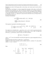
Fig 1 shows the control results for system (41) with constant time-delay via fuzzy controller (7)
with the previous gain matrices under the initial condition x
(t)=

20

T
, t ∈


−0.4909 0

.
0 2 4 6 8 10
−2
0
2
4
x
1
(t)
0 2 4 6 8 10
−1
0
1
2
x
2
(t)
0 2 4 6 8 10
−10
0
10
20
time (sec.)
u(t)
Fig. 1. Control results for system (41) without uncertainties and with constant time delay
τ
= 0.4909.

It is clear that the designed fuzzy controller can stabilize this system.
For the case of ΔA
i
= 0, ΔA
τi
= 0 and constant delay, the approaches in (Guan & Chen, 2004)
(Wu & Li, 2007) (Lin et al., 2006) cannot be used to design feedback controllers as the system
contains uncertainties. The method in (Chen & Liu, 2005b) and theorem 3 with λ
= 5canbe
used to design the fuzzy controllers. The corresponding results are listed below.
Methods Maximum allowed τ
Theorem of Chen and Liu (Chen & Liu, 2005a) 0.1498
Theorem 3 0.4770
Table 2. Comparison Among Various Delay-Dependent Stabilization Methods With
uncertainties
It appears from Table 2 that our result improves the existing ones in the case of uncertain T-S
fuzzy model with constant time-delay.
For the case of uncertain T-S fuzzy model with time-varying delay, the approaches proposed
in (Guan & Chen, 2004) (Chen & Liu, 2005a) (Wu & Li, 2007) (Chen et al., 2007) and (Lin et al.,
2006) cannot be used to design feedback controllers as the system contains uncertainties and
time-varying delay. By using theorem 3 with the choice of λ
= 5, τ(t)=0.25 + 0.15 sin(t)(τ =
0.4, β = 0.15), we can obtain the following state-feedback gain matrices:
K
1
=

4.7478
−13.5217


, K
2
=

3.1438
−13.2255

31
Robust Control of Nonlinear Time-Delay Systems via Takagi-Sugeno Fuzzy Models
12 Will-be-set-by-IN-TECH
The simulation was tested under the initial conditions x(t)=

20

T
, t ∈

−0.4 0

and
uncertainty F
(t)=

sin
(t) 0
0cos
(t)

.
0 2 4 6 8 10

−2
0
2
4
x
1
(t)
0 2 4 6 8 10
−1
0
1
2
x
2
(t)
0 2 4 6 8 10
−5
0
5
10
time (sec.)
u(t)
Fig. 2. Control results for system (41) with uncertainties and with time varying-delay
τ
(t)=0.25 + 0.15sin(t)
From the simulation results in figure 2, it can be clearly seen that our method offers a
new approach to stabilize nonlinear systems represented by uncertain T-S fuzzy model with
time-varying delay.
The second example illustrates the validity of the design method in the case of slow time
varying delay (β

< 1)
4.2 Example 2: Application to control a truck-trailer
In this example, we consider a continuous-time truck-trailer system, as shown in Fig. 3.
We will use the delayed model given by (Chen & Liu, 2005a). It is assumed that τ
(t)=1.10 +
0.75 sin( t). Obviously, we have τ = 1.85, β = 0.75. The time-varying delay model with
uncertainties is given by
˙
x
(t)=
2
∑
i=1
h
i
(x
1
(t))[ (A
i
+ ΔA
i
)x(t)+(A
τi
+ ΔA
τi
)x(t − τ(t)) + (B
i
+ ΔB
i
)u(t)] (43)

where
A
1
=
⎡
⎢
⎢
⎣
−a
vt
Lt
0
00
a
vt
Lt
0
00
a
v
2
t
2
2Lt
0
vt
t
0
0
⎤

⎥
⎥
⎦
, A
τ1
=
⎡
⎢
⎢
⎣
−(1 −a)
vt
Lt
0
00
(1 − a)
vt
Lt
0
00
(1 − a)
v
2
t
2
2Lt
0
00
⎤
⎥

⎥
⎦
A
2
=
⎡
⎢
⎢
⎣
−a
vt
Lt
0
00
a
vt
Lt
0
00
a
dv
2
t
2
2Lt
0
dvt
t
0
0

⎤
⎥
⎥
⎦
, A
τ2
=
⎡
⎢
⎢
⎣
−(1 −a)
vt
Lt
0
00
(1 − a)
vt
Lt
0
00
(1 − a)
dv
2
t
2
2Lt
0
00
⎤

⎥
⎥
⎦
32
Recent Advances in Robust Control – Novel Approaches and Design Methods
Robust Control of Nonlinear Time-Delay Systems via Takagi-Sugeno Fuzzy Models 13
x
0
x
3
(+)
x
3
(−)
x
2
x
0
u
u
x
1
l
L
Fig. 3. Truck-trailer system
B
1
= B
2
=


vt
lt
0
00

T
ΔA
1
= ΔA
2
= ΔA
τ1
= ΔA
τ2
= MF(t)E
with
M
=

0.255 0.255 0.255

T
, E =

0.1 0 0

ΔB
1
= ΔB

2
= M
b
F(t)E
b
with
M
b
=

0.1790 0 0

T
, E
b1
= 0.05, E
b2
= 0.15
where
l
= 2.8, L = 5.5, v = −1, t = 2, t
0
= 0.5, a = 0.7, d =
10t
0
π
The membership functions are defined as
h
1
(θ(t)) = (1 −

1
1 + ex p(−3(θ(t) −0.5π))
) ×(
1
1 + ex p(−3(θ(t)+0.5π))
)
h
2
(θ(t)) = 1 −h
1
where
θ
(t)=x
2
(t)+a(vt /2L)x
1
(t)+(1 −a)(vt/2L)x
1
(t − τ(t))
By using theorem 3, with the choice of λ = 5, we can obtain the following feasible solution:
P
=
⎡
⎣
0.2249 0.0566
−0.0259
0.0566 0.0382 0.0775
−0.0259 0.0775 2.7440
⎤
⎦

, S
=
⎡
⎣
0.2408
−0.0262 −0.1137
−0.0262 0.0236 0.0847
−0.1137 0.0847 0.3496
⎤
⎦
33
Robust Control of Nonlinear Time-Delay Systems via Takagi-Sugeno Fuzzy Models
14 Will-be-set-by-IN-TECH
Z =
⎡
⎣
0.0373 0.0133
−0.0052
0.0133 0.0083 0.0202
−0.0052 0.0202 1.0256
⎤
⎦
, T
=
⎡
⎣
0.0134 0.0053 0.0256
0.0075 0.0038
−0.0171
0.0001 0.0014 0.0642

⎤
⎦
Y
=
⎡
⎣
−0.0073 −0.0022 0.0192
−0.0051 −0.0031 0.0096
0.0012
−0.0012 −0.0804
⎤
⎦

A1
= 0.1087, 
A2
= 0.0729, 
A12
= 0.1184

Aτ1
= 0.0443, 
Aτ2
= 0.0369, 
Aτ12
= 0.0432

B1
= 0.3179, 
B2

= 0.3383, 
B12
= 0.3250
K
1
=

3.7863
−5.7141 0.1028

K
2
=

3.8049
−5.8490 0.0965

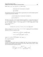
The simulation was carried out for an initial condition x
(t)=

−0.5π 0.75π −5

T
, t ∈

−1.85 0

.
0 10 20 30 40 50
−5

0
5
x
1
(t)
0 10 20 30 40 50
−5
0
5
x
2
(t)
0 10 20 30 40 50
−20
−10
0
x
3
(t)
0 10 20 30 40 50
−50
0
50
time (sec.)
u(t)
Fig. 4. Control results for the truck-trailer system (41)
The third example is presented to illustrate the effectiveness of the proposed main result for
fast time-varying delay system.
4.3 Example 3: Application to an inverted pendulum
Consider the well-studied example of balancing an inverted pendulum on a cart (Cao et al.,

2000).
˙
x
1
= x
2
(44)
˙
x
2
=
g sin(x
1
) − amlx
2
2
sin(2x
1
)/2 − a cos(x
1
)u
4l/3 −aml cos
2
(x
1
)
(45)
34
Recent Advances in Robust Control – Novel Approaches and Design Methods
Robust Control of Nonlinear Time-Delay Systems via Takagi-Sugeno Fuzzy Models 15

(M)
u(t)
θ
(m)
Fig. 5. Inverted pendulum
where x
1
is the pendulum angle (represented by θ in Fig. 5), and x
2
is the angular velocity (
˙
θ).g
= 9.8m/s
2
is the gravity constant , m is the mass of the pendulum, M is the mass of the
cart, 2l is the length of the pendulum and u is the force applied to the cart. a
= 1/(m + M).
The nonlinear system can be described by a fuzzy model with two IF-THEN rules:
Plant Rule 1: IF x
1
is about 0, Then
˙
x
(t)=A
1
x(t)+B
1
u(t) (46)
Plant rule 2: IF x
1

is about ±
π
2
,Then
˙
x
(t)=A
2
x(t)+B
2
u(t) (47)
where
A
1
=

01
17.2941 0

, A
2
=

01
12.6305 0

B
1
=


0
−0.1765

, B
2
=

0
−0.0779

The membership functions are
h
1
=(1 −
1
1 + exp(−7(x
1
−π/4))
) ×(
1 +
1
1 + exp(−7(x
1
+ π/4))
)
h
2
= 1 −h
1
In order to illustrate the use of theorem (3), we assume that the delay terms are perturbed

along values of the scalar s
∈ [0, 1], and the fuzzy time-delay model considered here is as
follows:
˙
x
(t)=
r
∑
i=1
h
i
[((1 −s)A
i
+ ΔA
i
)x(t)+(sA
τi
+ ΔA
τi
)x(t −τ(t)) + B
i
u(t)] (48)
where
A
1
=

01
17.2941 0


, A
2
=

01
12.6305 0

B
1
=

0
−0.1765

, B
2
=

0
−0.0779

ΔA
1
= ΔA
2
= ΔA
τ1
= ΔA
τ2
= MF(t)E

35
Robust Control of Nonlinear Time-Delay Systems via Takagi-Sugeno Fuzzy Models
16 Will-be-set-by-IN-TECH
with
M
=

0.1 0
00.1

T
, E =

0. 0
00.1

Let s
= 0.1 and uncertainty F(t)=

sin
(t) 0
0cos
(t)

. We consider a fast time-varying delay
τ
(t)=0.2 + 1.2
|
sin(t)
|

(β = 1.2 > 1).
Using LMI-TOOLBOX, there is a set of feasible solutions to LMIs (29).
K
1
=

159.7095 30.0354

, K
2
=

347.2744 78.5552

Fig. 4 shows the control results for the system (48) with time-varying delay τ
(t)=0.2 +
1.2
|
sin(t)
|
under the initial condition x(t)=

20

T
, t ∈

−1.40 0

.

0 2 4 6 8 10
−1
0
1
2
x
1
(t)
0 2 4 6 8 10
−4
−2
0
2
x
2
(t)
0 2 4 6 8 10
−500
0
500
1000
time (sec.)
u(t)
Fig. 6. Control results for the system (48) with time-varying delayτ(t)=0.2 + 1.2
|
sin(t)
|
.
5. Conclusion
In this chapter, we have investigated the delay-dependent design of state feedback stabilizing

fuzzy controllers for uncertain T-S fuzzy systems with time varying delay. Our method is
an important contribution as it establishes a new way that can reduce the conservatism and
the computational efforts in the same time. The delay-dependent stabilization conditions
obtained in this chapter are presented in terms of LMIs involving a single tuning parameter.
Finally, three examples are used to illustrate numerically that our results are less conservative
than the existing ones.
6. References
Boukas, E. & ElHajjaji, A. (2006). On stabilizability of stochastic fuzzy systems, American
Control Conference, 2006, Minneapolis, Minnesota, USA, pp. 4362–4366.
36
Recent Advances in Robust Control – Novel Approaches and Design Methods
Robust Control of Nonlinear Time-Delay Systems via Takagi-Sugeno Fuzzy Models 17
Cao, S. G., Rees, N. W. & Feng, G. (2000). h
∞
control of uncertain fuzzy continuous-time
systems, Fuzzy Sets and Systems Vol. 115(No. 2): 171–190.
Cao, Y Y. & Frank, P. M. (2000). Analysis and synthesis of nonlinear timedelay systems via
fuzzy control approach, IEEE Transactions on Fuzzy Systems Vol. 8(No. 12): 200–211.
Chadli, M. & ElHajjaji, A. (2006). A observer-based robust fuzzy control of nonlinear systems
with parametric uncertaintie, Fuzzy Sets and Systems Vol. 157(No. 9): 1279–1281.
Chen, B., Lin, C., Liu, X. & Tong, S. (2008). Guarateed cost control of t-s fuzzy systems with
input delay, International Journal Robust Nonlinear Control Vol. 18: 1230–1256.
Chen, B. & Liu, X. (2005a). Delay-dependent robust h
∞
control for t-s fuzzy systems with time
delay, IEEE Transactions on Fuzzy Systems Vol. 13(No. 4): 544 – 556.
Chen, B. & Liu, X. (2005b). Fuzzy guaranteed cost control for nonlinear systems with
time-varying delay, Fuzzy sets and systems Vol. 13(No. 2): 238 – 249.
Chen, B., Liu, X., Tang, S. & Lin, C. (2008). Observer-based stabilization of t-s fuzzy systems
with input delay, IEEE Transactions on fuzzy systems Vol. 16(No. 3): 625–633.

Chen, B., Liu, X. & Tong, S. (2007). New delay-dependent stabilization conditions of t-s fuzzy
systems with constant delay, Fuzzy sets and systems Vol. 158(No. 20): 2209 – 2242.
Guan, X P. & Chen, C L. (2004). Delay-dependent guaranteed cost control for t-s fuzzy
systems with time delays, IEEE Transactions on Fuzzy Systems Vol. 12(No. 2): 236–249.
Guerra, T., Kruszewski, A., Vermeiren, L. & Tirmant, H. (2006). Conditions of output
stabilization for nonlinear models in the takagi-sugeno’s form, Fuzzy Sets and Systems
Vol. 157(No. 9): 1248–1259.
He, Y., Wang, Q., Xie, L. H. & Lin, C. (2007). Further improvement of free-weighting matrices
technique for systems with time-varying delay, IEEE Trans. Autom. Control Vol. 52(No.
2): 293–299.
He, Y., Wu, M., She, J. H. & Liu, G. P. (2004). Parameter-dependent lyapunov functional for
stability of time-delay systems with polytopic type uncertainties, IEEE Trans. Autom.
Control Vol. 49(No. 5): 828–832.
Kim, E. & Lee, H. (2000). New approaches to relaxed quadratic stability condition of fuzzy
control systems, IEEE Transactions on Fuzzy Systems Vol. 8(No. 5): 523–534.
Li, C., Wang, H. & Liao, X. (2004). Delay-dependent robust stability of uncertain fuzzy
systems with time-varying delays, Control Theory and Applications, IEE Proceedings,
IET, pp. 417–421.
Lin, C., Wang, Q. & Lee, T. (2006). Delay-dependent lmi conditions for stability and
stabilization of t-s fuzzy systems with bounded time-delay, Fuzzy sets and systems
Vol. 157(No. 9): 1229 – 1247.
Moon, Y. S., Park, P., Kwon, W. H. & Lee, Y. S. (2001). Delay-dependent robust
stabilization of uncertain state-delayed systems, International Journal of control Vol.
74(No. 14): 1447–1455.
Oudghiri, M., Chadli, M. & ElHajjaji, A. (2007). One-step procedure for robust output fuzzy
control, CD-ROM of the 15th Mediterranean Conference on Control and Automation,
IEEE-Med’07, Athens, Greece, pp. 1 – 6.
Park, P., Lee, S. S. & Choi, D. J. (2003). A state-feedback stabilization for nonlinear
time-delay systems: A new fuzzy weighting-dependent lyapunov-krasovskii
functional approach, Proceedings of the 42nd IEEE Conference on Decision and Control,

Maui, Hawaii, pp. 5233–5238.
37
Robust Control of Nonlinear Time-Delay Systems via Takagi-Sugeno Fuzzy Models
18 Will-be-set-by-IN-TECH
Wang, H. O., Tanaka, K. & Griffin, M. F. (1996). An approach to fuzzy control of nonlinear
systems: Stability and design issues, IEEE Transactions on fuzzy systems Vol. 4 (N o.
1): 14–23.
Wang, Y., Xie, L. & Souza, C. D. (1992). Robust control of a class of uncertain nonlinear
systems, Systems control letters Vol. 19(No. 2): 139 – 149.
Wu, H N. & Li, H X. (2007). New approach to delay-dependent stability analysis and
stabilization for continuous-time fuzzy systems with time-varying delay, IEEE
Transactions on Fuzzy Systems Vol. 15(No. 3): 482–493.
Wu, M., He, Y. & She, J. (2004). New delay-dependent stability criteria and stabilizing method
for neutral systems, IEEE transactions on automatic control Vol. 49(No. 12): 2266–2271.
Xie, L. & DeSouza, C. (1992). Robust h
∞
control for linear systems with norm-bounded
time-varying uncertainty, IEEE Trans. Automatic Control Vol. 37(No. 1): 1188 – 1191.
Zhang, Y. & Heng, P. (2002). Stability of fuzzy control systems with bounded uncertain delays,
IEEE Transactions on Fuzzy Systems Vol. 10(No. 1): 92–97.
38
Recent Advances in Robust Control – Novel Approaches and Design Methods
3
Observer-Based Robust Control of Uncertain
Fuzzy Models with Pole Placement Constraints
Pagès Olivier and El Hajjaji Ahmed
University of Picardie Jules Verne, MIS, Amiens
France
1. Introduction
Practical systems are often modelled by nonlinear dynamics. Controlling nonlinear systems

are still open problems due to their complexity nature. This problem becomes more complex
when the system parameters are uncertain. To control such systems, we may use the
linearization technique around a given operating point and then employ the known
methods of linear control theory. This approach is successful when the operating point of
the system is restricted to a certain region. Unfortunately, in practice this approach will not
work for some physical systems with a time-varying operating point. The fuzzy model
proposed by Takagi-Sugeno (T-S) is an alternative that can be used in this case. It has been
proved that T-S fuzzy models can effectively approximate any continuous nonlinear
systems by a set of local linear dynamics with their linguistic description. This fuzzy
dynamic model is a convex combination of several linear models. It is described by fuzzy
rules of the type If-Then that represent local input output models for a nonlinear system. The
overall system model is obtained by “blending” these linear models through nonlinear
fuzzy membership functions. For more details on this topic, we refer the reader to (Tanaka
& al 1998 and Wand & al, 1995) and the references therein.
The stability analysis and the synthesis of controllers and observers for nonlinear systems
described by T-S fuzzy models have been the subject of many research works in recent
years. The fuzzy controller is often designed under the well-known procedure: Parallel
Distributed Compensation (PDC). In presence of parametric uncertainties in T-S fuzzy
models, it is necessary to consider the robust stability in order to guarantee both the stability
and the robustness with respect to the latter. These may include modelling error, parameter
perturbations, external disturbances, and fuzzy approximation errors. So far, there have
been some attempts in the area of uncertain nonlinear systems based on the T-S fuzzy
models in the literature. The most of these existing works assume that all the system states
are measured. However, in many control systems and real applications, these are not always
available. Several authors have recently proposed observer based robust controller design
methods considering the fact that in real control problems the full state information is not
always available. In the case without uncertainties, we apply the separation property to
design the observer-based controller: the observer synthesis is designed so that its dynamics
are fast and we independently design the controller by imposing slower dynamics. Recently,
much effort has been devoted to observer-based control for T-S fuzzy models. (Tanaka & al,

1998) have studied the fuzzy observer design for T-S fuzzy control systems. Nonetheless, in

Recent Advances in Robust Control – Novel Approaches and Design Methods

40
the presence of uncertainties, the separation property is not applicable any more. In (El
Messousi & al, 2006), the authors have proposed sufficient global stability conditions for the
stabilization of uncertain fuzzy T-S models with unavailable states using a robust fuzzy
observer-based controller but with no consideration to the control performances and in
particular to the transient behaviour.
From a practical viewpoint, it is necessary to find a controller which will specify the desired
performances of the controlled system. For example, a fast decay, a good damping can be
imposed by placing the closed-loop poles in a suitable region of the complex plane. Chilali
and Gahinet (Chilali & Gahinet, 1996) have proposed the concept of an LMI (Linear Matrix
Inequality) region as a convenient LMI-based representation of general stability regions for
uncertain linear systems. Regions of interest include α-stability regions, disks and conic
sectors. In (Chilali & al 1999), a robust pole placement has been studied in the case of linear
systems with static uncertainties on the state matrix. A vertical strip and α-stability robust
pole placement has been studied in (Wang & al, 1995, Wang & al, 1998 and Wang & al, 2001)
respectively for uncertain linear systems in which the concerned uncertainties are polytopic
and the proposed conditions are not LMI. In (Hong & Man 2003), the control law synthesis
with a pole placement in a circular LMI region is presented for certain T-S fuzzy models.
Different LMI regions are considered in (Farinwata & al, 2000 and Kang & al, 198), for
closed-loop pole placements in the case of T-S fuzzy models without uncertainties.
In this work, we extend the results of (El Messoussi & al, 2005), in which we have developed
sufficient robust pole placement conditions for continuous T-S fuzzy models with
measurable state variables and structured parametric uncertainties.
The main goal of this paper is to study the pole placement constraints for T-S fuzzy models
with structured uncertainties by designing an observer-based fuzzy controller in order to
guarantee the closed-loop stability. However, like (Lo & Li, 2004 and Tong & Li, 2002), we do

not know the position of the system state poles as well as the position of the estimation error
poles. The main contribution of this paper is as follows: the idea is to place the poles associated
with the state dynamics in one LMI region and to place the poles associated with the
estimation error dynamics in another LMI region (if possible, farther on the left). However, the
separation property is not applicable unfortunately. Moreover, the estimation error dynamics
depend on the state because of uncertainties. If the state dynamics are slow, we will have a
slow convergence of the estimation error to the equilibrium point zero in spite of its own fast
dynamics. So, in this paper, we propose an algorithm to design the fuzzy controller and the
fuzzy observer separately by imposing the two pole placements. Moreover, by using the H
∞

approach, we ensure that the estimation error converges faster to the equilibrium point zero.
This chapter is organized as follows: in Section 2, we give the class of uncertain fuzzy
models, the observer-based fuzzy controller structure and the control objectives. After
reviewing existing LMI constraints for a pole placement in Section 3, we propose the new
conditions for the uncertain augmented T-S fuzzy system containing both the fuzzy
controller as well as the observer dynamics. Finally, in Section 4, an illustrative application
example shows the effectiveness of the proposed robust pole placement approach. Some
conclusions are given in Section 5.
2. Problem formulation and preliminaries
Considering a T-S fuzzy model with parametric uncertainties composed of r plant rules that
can be represented by the following fuzzy rule:

Observer-Based Robust Control of Uncertain Fuzzy Models with Pole Placement Constraints

41
Plant rule i :
If
1
()ztis M

1i
and …and ()zt
ν
is
i
M
ν
Then
() ( )() ( )(),
() () 1, ,
ii ii
i
xt A A xt B B ut
yt Cxt i r
=+Δ ++Δ
⎧
⎨
==
⎩

(1)
The structured uncertainties considered here are norm-bounded in the form:

() ,
() , 1, ,
iaiaiai
ibibibi
AH tE
BH tEi r
Δ= Δ

Δ= Δ =
(2)
Where
,,,
ai bi ai bi
HHEEare known real constant matrices of appropriate dimension, and
(), ()
ai bi
ttΔΔ
are unknown matrix functions satisfying:

() () ,
() () 1, ,
t
ai ai
t
bi bi
ttI
ttIi r
ΔΔ ≤
ΔΔ ≤ =
(3)
()
t
ai
tΔ is the transposed matrix of ()
ai
t
Δ
and I is the matrix identity of appropriate

dimension. We suppose that pairs
(
)
,
ii
A
B are controllable and
(
)
,
ii
A
C are observable.
i
j
M

indicates the
j
th
fuzzy set associated to the i
th
variable ()
i
zt, r is the number of fuzzy model
rules,
()
n
xt ∈ℜ
is the state vector,

()
m
ut
∈
ℜ
is the input vector,
()
l
y
tR∈
is the output vector,
nn
i
A
×
∈ℜ ,
nm
i
B
×
∈ℜ and
ln
i
C
×
∈ℜ .
1
(), , ()
v
zt zt are premise variables.

From (1), the T-S fuzzy system output is :

[]
1
1
() (())( )() ( )()
() (()) ()
r
iiiii
i
r
ii
i
xt h zt A A xt B B ut
yt h zt Cxt
=
=
⎧
=+Δ++Δ
∑
⎪
⎪
⎨
⎪
=
∑
⎪
⎩

(4)

where
1
(())
(())
(())
i
i
r
i
i
wzt
hzt
wzt
=
=
∑
and
1
( ( )) ( ( ))
ij
v
iMj
j
wzt zt
μ
=
=
∏

Where

(())
ij
Mj
zt
μ
is the fuzzy meaning of symbol M
ij
.
In this paper we assume that all of the state variables are not measurable. Fuzzy state
observer for T-S fuzzy model with parametric uncertainties (1) is formulated as follows:
Observer rule i:
If
1
()zt
is M
1i
and …and
()zt
ν
is
i
M
ν
Then
ˆˆ ˆ
() () () ( () ()),
ˆˆ
() () 1, ,
ii i
i

xt Axt But G yt yt
yt Cxt i r
⎧
=+− −
⎪
⎨
==
⎪
⎩

(5)
The fuzzy observer design is to determine the local gains
nl
i
G
×
∈ℜ in the consequent part.
Note
that the premise variables do not depend on the state variables estimated by a fuzzy
observer.
The output of (5) is represented as follows:

Recent Advances in Robust Control – Novel Approaches and Design Methods

42

{}
1
1
ˆˆ ˆ

() (()) () () ( () ())
ˆˆ
() (()) ()
r
iiii
i
r
ii
i
xt h zt Axt But G
y
t
y
t
yt h zt Cxt
=
=
⎧
=+−−
⎪
⎪
⎨
⎪
=
⎪
⎩
∑
∑

(6)

To stabilize this class of systems, we use the PDC observer-based approach (Tanaka & al,
1998). The PDC observer-based controller is defined by the following rule base system:
Controller rule i :
If
1
()ztis M
1i
and …and ()zt
ν
is
i
M
ν
Then
ˆ
() () 1, ,
i
ut Kxt i r
=
= (7)
The overall fuzzy controller is represented by:

1
1
1
ˆ
(()) ()
ˆ
() (()) ()
(())

r
ii
r
i
ii
r
i
i
i
wztKxt
ut h zt Kxt
wzt
=
=
=
==
∑
∑
∑
(8)
Let us denote the estimation error as:

ˆ
() () ()et xt xt
=−
(9)
The augmented system containing both the fuzzy controller and observer is represented as
follows:

() ()

(())
() ()
xt xt
Azt
et et
⎡
⎤⎡⎤
=×
⎢
⎥⎢⎥
⎣
⎦⎣⎦


(10)
where

()( )
11
( ( )) ( ( )) ( ( ))
( )() ()
rr
ij ij
ij
iiiij iij
ij
ii
j
ii
j

i
j
Azt h zt h zt A
AABBK BBK
A
ABK AGC BK
==
=
+Δ + +Δ − +Δ
⎡
⎤
⎢
⎥
=
Δ+Δ + −Δ
⎢
⎥
⎣
⎦
∑∑
(11)
The main goal is first, to find the sets of matrices
i
K and
i
G in order to guarantee the global
asymptotic stability of the equilibrium point zero of (10) and secondly, to design the fuzzy
controller and the fuzzy observer of the augmented system (10) separately by assigning both
“observer and controller poles” in a desired region in order to guarantee that the error
between the state and its estimation converges faster to zero. The faster the estimation error

will converge to zero, the better the transient behaviour of the controlled system will be.
3. Main results
Given (1), we give sufficient conditions in order to satisfy the global asymptotic stability of
the closed-loop for the augmented system (10).

Observer-Based Robust Control of Uncertain Fuzzy Models with Pole Placement Constraints

43
Lemma 1:
The equilibrium point zero of the augmented system described by (10) is globally
asymptotically stable if there exist common positive definite matrices
1
P and
2
P , matrices
i
W ,
j
V and positive scalars 0
ij
ε
 such as

0, 1, ,
0,
ii
ij ji
ir
ijr
Π≤ =

Π
+Π ≤ < ≤
(12)
And

0, 1, ,
0,
ii
ij ji
ir
ijr
Σ≤ =
Σ
+Σ ≤ < ≤
(13)
with
1
1
0.5 0 0 0
00.5 00
00 0
000
ttt
i
j
ai
j
bi i bi
ai ij
bi j ij

ij
t
iij
t
bi i
j
DPEVE BH
EP I
EV I
BI
HI
ε
ε
ε
ε
⎡⎤
⎢⎥
−
⎢⎥
⎢⎥
−
Π=
⎢⎥
⎢⎥
−
⎢⎥
⎢⎥
−
⎢⎥
⎣⎦

*
22
1
1
2
1
2
1
000
000
000.5 0
00 0
tt t
ij j bi ai bi j
bi j ij
t
ij
ai ij
t
bi ij
jij
DKEPH PH K
EK I
HP I
HP I
KI
ε
ε
ε
ε

−
−
−
−
⎡
⎤
⎢
⎥
⎢
⎥
−
⎢
⎥
⎢
⎥
∑=
−
⎢
⎥
⎢
⎥
−
⎢
⎥
⎢
⎥
−
⎣
⎦

11
*1
22
ttttt
i
j
iii
jj
ii
j
ai ai i
j
bi bi
ttttt
ij i i i j j i ij j bi bi j
DAPPABVVB HH HH
DPAAPWCCW KEEK
εε
ε
−
=++++ +
=++ + +

Proof: using theorem 7 in (Tanaka & al, 1998), property (3), the separation lemma (Shi & al,
1992)) and the Schur’s complement (Boyd & al, 1994), the above conditions (12) and (13)
hold with some changes of variables. Let us briefly explain the different steps…
From (11), in order to ensure the global, asymptotic stability, the sufficient conditions must
be verified:

0: ( , ) 0

t
t
ij ij
D
XX MAX AXXA
∃
=> = + < (14)
Let:
11
22
0
0
X
X
X
⎡⎤
=
⎢⎥
⎣⎦
where 0 is a zero matrix of appropriate dimension. From (14), we have:

12
(,)
DDD
M
AX M M=+ (15)
With
1
1
2

0
0
D
D
M
D
⎡⎤
=
⎢⎥
⎣⎦
where

11111 1111
ttt
iii
jj
i
DAX XABKX XKB=++ + (16)
and

2 2222 2222
ttt
iii
jj
i
DAX XAGCX XCG=++ + (17)