Recent Advances in Signal Processing 2011 Part 11 ppt

Estimation of the instantaneous harmonic parameters of speech 337

b)
c)
Fig. 8. Harmonic parameters estimation: a) source signal; b) estimated deterministic part;
c) estimated stochastic part

An example of harmonic analysis is presented in Figure 8(a). The source signal is a phrase
uttered by a male speaker (ܨ
௦
ൌ ͺkHz). The deterministic part of the signal Figure 8(b) was
synthesized using estimated harmonic parameters and subtracted from the source in order
to get the stochastic part Figure 9(c). The spectrograms show that all steady harmonics of the
source are modelled by sinusoidal representation when the residual part contains transient
and noise components.

7.2 Harmonic analysis in TTS systems
This subsection presents an experimental application of sinusoidal modelling with proposed
analysis techniques to a TTS system. Despite the fact that many different techniques have
been proposed, segment concatenation is still the major approach to speech synthesis. The
speech segments (allophones) are assembled into synthetic speech and this process involves
time-scale and pitch-scale modifications in order to produce natural-like sounds. The
concatenation can be carried out either in time or frequency domain. Most time domain
techniques are similar to the Pitch-Synchronous Overlap and Add method (PSOLA)
(Moulines and Charpentier, 1990). The speech waveform is separated into short-time signals
by the analysis pitch-marks (that are defined by the source pitch contour) and then
processed and joined by the synthesis pitch-marks (that are defined by the target pitch
contour). The process requires accurate pitch estimation of the source waveform. Placing

c)
d)

Fig. 7. Frame analysis by autocorrelation and sinusoidal parameters conversion: a)
autocorrelation spectrum estimation; b) autocorrelation residual; c) instantaneous LPC
spectrum; d) instantaneous residual

7. Experimental applications

The described methods of sinusoidal and harmonic analysis can be used in several speech
processing systems. This section presents some application results.

7.1 Application of harmonic analysis to parametric speech coding
Accurate estimation of sinusoidal parameters can significantly improve performance of
coding systems. Well-known compressing algorithms that use sinusoidal representation
may benefit from fine accurate harmonic/residual separation, providing higher quality of
the decoded signal. The described analysis technique has been applied to hybrid speech and
audio coding (Petrovsky et al., 2008).


a)
Recent Advances in Signal Processing338


e)

f)
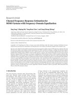
Fig. 9. Segment analysis: a) source waveform segment; b) estimated fundamental
frequency contour; c) estimated harmonic amplitudes; d) estimated stochastic part; e)
spectrogram of the source segment; f) spectrogram of the stochastic part

The periodical signal  with pitch shifting can be synthesized from its parametric
representation as follows:






 















(46)
Phases of harmonic components 




are calculated according to the new fundamental
frequency contour 



:






 




















(47)

Harmonic frequencies are calculated by the formula (3):






 








(48)
Additional phase difference 





is used in order to maintain relative phases of harmonics
and the fundamental:








 




 






(49)
In synthesis process the phase differences 





are good substitutions of phase parameters





since all the harmonics are kept coordinated regardless of the frequency contour and
the initial phase of the fundamental.
Due to parametric representation spectral amplitude and phase mismatches at segments

borders can be efficiently smoothed. Spectral amplitudes of acoustically related sounds can
be matched by simultaneous fading out and in that is equivalent to linear spectral
smoothing (Dutoit 1997). Phase discontinuities are also can be matched by linear laws
taking into account that harmonic components are represented by their relative phases






. However, large discontinuities (when absolute difference exceeds ) should be
eliminated by adding multiplies of  to the phase parameters of the next segment. Thus,
phase parameters are smoothed in the same way as spectral amplitudes, providing
imperceptible concatenation of the segments.
In Figure 10 the proposed approach is compared with PSOLA synthesis, implemented as
described in (Moulines and Charpentier, 1990). A fragment of speech in Russian was
synthesized through two different techniques using the same source acoustic database. The

analysis pitch-marks is an important stage that significantly affects synthesis quality.
Frequency domain (parametric) techniques deal with frequency representations of the
segments instead of their waveforms what requires prior transformation of the acoustic
database to frequency domain. Harmonic modelling can be especially useful in TTS systems
for the following reasons:
- explicit control over pitch, tempo and timbre of the speech segments that insures
proper prosody matching ;
- high-quality segment concatenation can be performed using simple linear
smoothing laws;
- acoustic database can be highly compressed;
- synthesis can be implemented with low computational complexity.
In order to perform real-time synthesis in harmonic domain all waveform speech segments

should be analysed and stored in new database, which contains estimated harmonic
parameters and waveforms of stochastic signals. The analysis technique described in the
chapter can be used for parameterization. In Figure 9 a result of such parameterization is
presented. The analysed segment is sound [a:] of a female voice.
Speech concatenation with prosody matching can be efficiently implemented using
sinusoidal modelling. In order to modify durations of the segments the harmonic
parameters are recalculated at new instants, that are defined by some dynamic warping
function, the noise part is parameterized by spectral envelopes and then time-scaled as
described in (Levine and Smith, 1998).
Changing the pitch of a segment requires recalculation of harmonic amplitudes, maintaining
the original spectral envelope. Noise part of the segment is not affected by pitch shifting and
obviously should remain untouched. Let us consider the instantaneous frequency envelope
as a function ܧ
ሺ
݊ǡ ݂
ሻ
of two parameters (sample number and frequency respectively). After
harmonic parameterization the function is defined at frequencies of the harmonic
components that were calculated at the respective instants of time: ܧ൫݊ǡ ݂
௞
ሺ
݊
ሻ
൯ ൌ 
௞
ሺ
݊
ሻ
.
In order to get the completely defined function the piecewise-linear interpolation is used.

Such interpolation has low computational complexity and, at the same time, gives
sufficiently good approximation (Dutoit 1997).


a)

b)

c)

d)
Estimation of the instantaneous harmonic parameters of speech 339


e)

f)
Fig. 9. Segment analysis: a) source waveform segment; b) estimated fundamental
frequency contour; c) estimated harmonic amplitudes; d) estimated stochastic part; e)
spectrogram of the source segment; f) spectrogram of the stochastic part

The periodical signal  with pitch shifting can be synthesized from its parametric
representation as follows:





 
















(46)
Phases of harmonic components 




are calculated according to the new fundamental
frequency contour 


:







 




















(47)
Harmonic frequencies are calculated by the formula (3):







 








(48)
Additional phase difference 





is used in order to maintain relative phases of harmonics
and the fundamental:







 





 






(49)
In synthesis process the phase differences 





are good substitutions of phase parameters





since all the harmonics are kept coordinated regardless of the frequency contour and
the initial phase of the fundamental.
Due to parametric representation spectral amplitude and phase mismatches at segments
borders can be efficiently smoothed. Spectral amplitudes of acoustically related sounds can
be matched by simultaneous fading out and in that is equivalent to linear spectral
smoothing (Dutoit 1997). Phase discontinuities are also can be matched by linear laws
taking into account that harmonic components are represented by their relative phases







. However, large discontinuities (when absolute difference exceeds ) should be
eliminated by adding multiplies of  to the phase parameters of the next segment. Thus,
phase parameters are smoothed in the same way as spectral amplitudes, providing
imperceptible concatenation of the segments.
In Figure 10 the proposed approach is compared with PSOLA synthesis, implemented as
described in (Moulines and Charpentier, 1990). A fragment of speech in Russian was
synthesized through two different techniques using the same source acoustic database. The

analysis pitch-marks is an important stage that significantly affects synthesis quality.
Frequency domain (parametric) techniques deal with frequency representations of the
segments instead of their waveforms what requires prior transformation of the acoustic
database to frequency domain. Harmonic modelling can be especially useful in TTS systems
for the following reasons:
- explicit control over pitch, tempo and timbre of the speech segments that insures
proper prosody matching ;
- high-quality segment concatenation can be performed using simple linear
smoothing laws;
- acoustic database can be highly compressed;
- synthesis can be implemented with low computational complexity.
In order to perform real-time synthesis in harmonic domain all waveform speech segments
should be analysed and stored in new database, which contains estimated harmonic
parameters and waveforms of stochastic signals. The analysis technique described in the
chapter can be used for parameterization. In Figure 9 a result of such parameterization is
presented. The analysed segment is sound [a:] of a female voice.
Speech concatenation with prosody matching can be efficiently implemented using
sinusoidal modelling. In order to modify durations of the segments the harmonic
parameters are recalculated at new instants, that are defined by some dynamic warping

function, the noise part is parameterized by spectral envelopes and then time-scaled as
described in (Levine and Smith, 1998).
Changing the pitch of a segment requires recalculation of harmonic amplitudes, maintaining
the original spectral envelope. Noise part of the segment is not affected by pitch shifting and
obviously should remain untouched. Let us consider the instantaneous frequency envelope
as a function ܧ
ሺ
݊ǡ ݂
ሻ
of two parameters (sample number and frequency respectively). After
harmonic parameterization the function is defined at frequencies of the harmonic
components that were calculated at the respective instants of time: ܧ൫݊ǡ ݂
௞
ሺ
݊
ሻ
൯ ൌ 
௞
ሺ
݊
ሻ
.
In order to get the completely defined function the piecewise-linear interpolation is used.
Such interpolation has low computational complexity and, at the same time, gives
sufficiently good approximation (Dutoit 1997).


a)

b)

c)

d)
Recent Advances in Signal Processing340

The autocorrelation analysis was carried out with analysis frame 512 samples in length,
weighted by the Hamming window. Prediction order was 20 in both cases.


a)

b)

c)
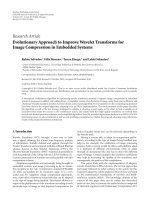
Fig. 11. Instantaneous formant analysis: a) source signal; b) autocorrelation analysis; c)
instantaneous LPC analysis

As can be seen from the pictures harmonic analysis with subsequent conversion into
prediction coefficients gives more localized formant trajectories. Some of them have more
complex form, however overall formant structure of the signal remains the same.

8. Conclusions

An estimation technique of instantaneous sinusoidal parameters has been presented in the
chapter. The technique is based on narrow-band filtering and can be applied to audio and
speech sounds. Signals with harmonic structure (such as voiced speech) can be analysed
using frequency-modulated filters with adjustable impulse response. The technique has a
good performance considering that accurate estimation is possible even in case of rapid
frequency modulations of pitch. A method of pitch detection and estimation has been

described as well. The use of filters with modulated impulse response, however, requires
precise estimation of instantaneous pitch that can be achieved through pitch values
recalculation during the analysis process. The main disadvantage of the method is high
computational cost in comparison with STFT.
Some experimental applications of the proposed approach have been illustrated. The
sinusoidal modelling based on the presented technique has been applied to speech coding,
and TTS synthesis with wholly satisfactory results.
The sinusoidal model can be used for estimation of LPC parameters that describe
instantaneous behaviour of the periodical signal. The presented conversion technique of
sinusoidal parameters into prediction coefficients provides high energy localization and
smaller residual for frequency-modulated signals, however overall performance entirely
depends on the quality of prior sinusoidal analysis. The instantaneous prediction

database segments were picked out from the speech of a female speaker. The sound sample
in Figure 10(a) is the result of the PSOLA method.

a)

b)
Fig. 10. TTS synthesis comparison: a) PSOLA synthesis; b) harmonic domain concatenation

In Figure 10(b) the sound sample is shown, that is the result of the described
analysis/synthesis approach. In order to get the parametric representation of the acoustic
database each segment was classified either as voiced or unvoiced. The unvoiced segments
were left untouched while the voiced were analyzed by the technique described in Section 4,
then prosody modifications and segment concatenation were carried out. Both sound
samples were synthesized at 22kHz, using the same predefined pitch contour.
As can be noticed from the presented samples the time domain concatenation approach
produces audible artefacts at segment borders. They are caused by phase and pitch
mismatching, that cannot be effectively avoided during synthesis. The described parametric

approach provides almost inaudible phase and pitch smoothing, without distorting spectral
and formant structure of the segments. The experiments have shown that this technique is
good enough even for short and fricative segments, however, the short Russian ‘r’ required
special adjustment of the filter parameters at the analysis stage in order to make proper
analysis of the segment.
The main drawback of the described approach is noise amplification immediately at
segment borders where the analysis filter gives less accurate results because of spectral
leakage. In the current experiment the problem was solved by fading out the estimated
noise part at segment borders. It is also possible to pick out longer segments at the database
preparation stage and then shorten them after parameterization.

7.3 Instantaneous LPC analysis of speech
LPC-based techniques are widely used for formant tracking in speech applications. Making
harmonic analysis first and then performing parameters conversion a higher accuracy of
formant frequencies estimation can be achieved. In Figure 11 a result of voiced speech
analysis is presented. The analysed signal (Figure 11(a)) is a vowel [a:] uttered by a male
speaker. This sound was sampled at 8kHz and analyzed by the autocorrelation (Figure
11(b)) and the harmonic conversion (Figure 11(c)) techniques. In order to give expressive
pictures prediction coefficients were updated for every sample of the signal in both cases.
Estimation of the instantaneous harmonic parameters of speech 341

The autocorrelation analysis was carried out with analysis frame 512 samples in length,
weighted by the Hamming window. Prediction order was 20 in both cases.


a)

b)

c)

Fig. 11. Instantaneous formant analysis: a) source signal; b) autocorrelation analysis; c)
instantaneous LPC analysis

As can be seen from the pictures harmonic analysis with subsequent conversion into
prediction coefficients gives more localized formant trajectories. Some of them have more
complex form, however overall formant structure of the signal remains the same.

8. Conclusions

An estimation technique of instantaneous sinusoidal parameters has been presented in the
chapter. The technique is based on narrow-band filtering and can be applied to audio and
speech sounds. Signals with harmonic structure (such as voiced speech) can be analysed
using frequency-modulated filters with adjustable impulse response. The technique has a
good performance considering that accurate estimation is possible even in case of rapid
frequency modulations of pitch. A method of pitch detection and estimation has been
described as well. The use of filters with modulated impulse response, however, requires
precise estimation of instantaneous pitch that can be achieved through pitch values
recalculation during the analysis process. The main disadvantage of the method is high
computational cost in comparison with STFT.
Some experimental applications of the proposed approach have been illustrated. The
sinusoidal modelling based on the presented technique has been applied to speech coding,
and TTS synthesis with wholly satisfactory results.
The sinusoidal model can be used for estimation of LPC parameters that describe
instantaneous behaviour of the periodical signal. The presented conversion technique of
sinusoidal parameters into prediction coefficients provides high energy localization and
smaller residual for frequency-modulated signals, however overall performance entirely
depends on the quality of prior sinusoidal analysis. The instantaneous prediction

database segments were picked out from the speech of a female speaker. The sound sample
in Figure 10(a) is the result of the PSOLA method.

a)

b)
Fig. 10. TTS synthesis comparison: a) PSOLA synthesis; b) harmonic domain concatenation

In Figure 10(b) the sound sample is shown, that is the result of the described
analysis/synthesis approach. In order to get the parametric representation of the acoustic
database each segment was classified either as voiced or unvoiced. The unvoiced segments
were left untouched while the voiced were analyzed by the technique described in Section 4,
then prosody modifications and segment concatenation were carried out. Both sound
samples were synthesized at 22kHz, using the same predefined pitch contour.
As can be noticed from the presented samples the time domain concatenation approach
produces audible artefacts at segment borders. They are caused by phase and pitch
mismatching, that cannot be effectively avoided during synthesis. The described parametric
approach provides almost inaudible phase and pitch smoothing, without distorting spectral
and formant structure of the segments. The experiments have shown that this technique is
good enough even for short and fricative segments, however, the short Russian ‘r’ required
special adjustment of the filter parameters at the analysis stage in order to make proper
analysis of the segment.
The main drawback of the described approach is noise amplification immediately at
segment borders where the analysis filter gives less accurate results because of spectral
leakage. In the current experiment the problem was solved by fading out the estimated
noise part at segment borders. It is also possible to pick out longer segments at the database
preparation stage and then shorten them after parameterization.

7.3 Instantaneous LPC analysis of speech
LPC-based techniques are widely used for formant tracking in speech applications. Making
harmonic analysis first and then performing parameters conversion a higher accuracy of
formant frequencies estimation can be achieved. In Figure 11 a result of voiced speech

analysis is presented. The analysed signal (Figure 11(a)) is a vowel [a:] uttered by a male
speaker. This sound was sampled at 8kHz and analyzed by the autocorrelation (Figure
11(b)) and the harmonic conversion (Figure 11(c)) techniques. In order to give expressive
pictures prediction coefficients were updated for every sample of the signal in both cases.
Recent Advances in Signal Processing342

McAulay, R. J. & Quateri T. F. (1992). The sinusoidal transform coder at 2400 b/s,
Proceedings of Military Communications Conference, Calif, USA, October 1992, San
Diego.
Moulines, E. & Charpentier, F. (1990). Pitch Synchronous Waveform Processing Techniques
for Text-to-Speech Synthesis Using Diphones. Speech Communication, Vol.9, No. 5-6,
(1990) 453-467.
Painter, T. & Spanias, A. (2003). Sinusoidal Analysis-Synthesis of Audio Using Perceptual
Criteria. EURASIP Journal on Applied Signal Processing, No. l, (2003) 15-20.
Petrovsky, A.; Stankevich, A. & Balunowski, J. (1999). The order tracking front-end
algorithms in the rotating machine monitoring systems based on the new digital
low order tracking, Proc. of the 6th Intern. Congress “On sound and vibration”,
pp.2985-2992, Denmark, 1999, Copenhagen.
Petrovsky, A.; Azarov, E. & Petrovsky, A. (2008). Harmonic representation and auditory
model-based parametric matching and its application in speech/audio analysis,
AES 126th Convention, Preprint 7705, Munich, Germany.
Rabiner, L. & Juang, B.H. (1993). Fundamentals of speech recognition, Prentice Hall, New
Jersey.
Serra, X. (1989). A system for sound analysis/transformation/synthesis based on a
deterministic plus stochastic decomposition, Ph.D. thesis, Stanford University,
Stanford, Calif, USA.
Spanias, A.S. (1994). Speech coding: a tutorial review. Proc. of the IEEE, Vol. 82, No. 10, (1994)
1541-1582.
Weruaga, L. & Kepesi, M. (2007). The fan-chirp transform for non-stationary harmonic
signals, Signal Processing, Vol. 87, issue 6, (June 2007) 1-18.

Zhang, F.; Bi, G. & Chen Y.Q. (2004). Harmonic transform, IEEE Proc Vis. Image Signal
Process., Vol. 151, No. 4, (August 2004) 257-264.

coefficients allow implementing fine formant tracking that can be useful in such applications
as speaker identification and speech recognition.
Future work is aimed at further investigation of the analysis filters and their behaviour,
finding optimized solutions for evaluation of sinusoidal parameters. It might be some
potential in adapting described methods to other applications such as vibration analyzer of
mechanical devices and diagnostics of throat diseases.

9. Acknowledgments

This work was supported by the Belarusian republican fund for fundamental research
under the grant T08MC-040 and the Belarusian Ministry of Education under the grant 09-
3102.

10. References

Abe, T.; Kobayashi, T. & Imai, S. (1995). Harmonics tracking and pitch extraction based on
instantaneous frequency, Proceedings of ICASSP 1995. pp. 756–759. 1995.
Azarov, E.; Petrovsky, A. & Parfieniuk, M. (2008). Estimation of the instantaneous harmonic
parameters of speech, Proceedings of the 16th European Signal Process. Conf.
(EUSIPCO-2008), CD-ROM, Lausanne, 2008.
Boashash, B. (1992). Estimating and interpreting the instantaneous frequency of a signal,
Proceedings of the IEEE, Vol. 80, No. 4, (1992) 520-568.
Dutoit, T. (1997). An Introduction to Text-to-speech Synthesis, Kluwer Academic Publishers, the
Netherlands.
Gabor, D. (1946). Theory of communication, Proc. IEE, Vol.93, No. 3, (1946) 429-457.
Gianfelici, F.; Biagetti, G.; Crippa, P. & Turchetti, C. (2007) Multicomponent AM–FM
Representations: An Asymptotically Exact Approach, IEEE Transactions on Audio,

Speech, and Language Processing, Vol. 15, No. 3, (March 2007) 823-837.
Griffin, D. & Lim, J. (1988). Multiband excitation vocoder, IEEE Trans. On Acoustics, Speech
and Signal Processing, Vol. 36, No. 8, (1988) 1223-1235.
Hahn, S. L. (1996) Hilbert Transforms in Signal Processing, MA: Artech House, Boston.
Huang, X; Acero, A. & Hon H.W. (2001). Spoken language processing, Prentice Hall, New
Jersey.
Levine, S. & Smith, J. (1998). A Sines+Transients+Noise Audio Representation for Data
Compression and Time/Pitch Scale Modifications, AES 105th Convention, Preprint
4781, San Francisco, CA, USA.
Maragos, P.; Kaiser, J. F. & Quatieri, T. F. (1993). Energy Separation in Signal Modulations
with Application to Speech Analysis”, IEEE Trans. On Signal Process., Vol. 41, No.
10, (1993) 3024-3051.
Markel J.D. & Gray A.H. (1976) Linear prediction of speech, Springer-Verlag Berlin Heidelberg,
New York.
McAulay, R. J. & Quatieri, T. F. (1986). Speech analysis/synthesis based on a sinusoidal
representation. IEEE Trans. On Acoustics, Speech and Signal Process., Vol. 34, No. 4,
(1986) 744-754.
Estimation of the instantaneous harmonic parameters of speech 343

McAulay, R. J. & Quateri T. F. (1992). The sinusoidal transform coder at 2400 b/s,
Proceedings of Military Communications Conference, Calif, USA, October 1992, San
Diego.
Moulines, E. & Charpentier, F. (1990). Pitch Synchronous Waveform Processing Techniques
for Text-to-Speech Synthesis Using Diphones. Speech Communication, Vol.9, No. 5-6,
(1990) 453-467.
Painter, T. & Spanias, A. (2003). Sinusoidal Analysis-Synthesis of Audio Using Perceptual
Criteria. EURASIP Journal on Applied Signal Processing, No. l, (2003) 15-20.
Petrovsky, A.; Stankevich, A. & Balunowski, J. (1999). The order tracking front-end
algorithms in the rotating machine monitoring systems based on the new digital
low order tracking, Proc. of the 6th Intern. Congress “On sound and vibration”,

pp.2985-2992, Denmark, 1999, Copenhagen.
Petrovsky, A.; Azarov, E. & Petrovsky, A. (2008). Harmonic representation and auditory
model-based parametric matching and its application in speech/audio analysis,
AES 126th Convention, Preprint 7705, Munich, Germany.
Rabiner, L. & Juang, B.H. (1993). Fundamentals of speech recognition, Prentice Hall, New
Jersey.
Serra, X. (1989). A system for sound analysis/transformation/synthesis based on a
deterministic plus stochastic decomposition, Ph.D. thesis, Stanford University,
Stanford, Calif, USA.
Spanias, A.S. (1994). Speech coding: a tutorial review. Proc. of the IEEE, Vol. 82, No. 10, (1994)
1541-1582.
Weruaga, L. & Kepesi, M. (2007). The fan-chirp transform for non-stationary harmonic
signals, Signal Processing, Vol. 87, issue 6, (June 2007) 1-18.
Zhang, F.; Bi, G. & Chen Y.Q. (2004). Harmonic transform, IEEE Proc Vis. Image Signal
Process., Vol. 151, No. 4, (August 2004) 257-264.

coefficients allow implementing fine formant tracking that can be useful in such applications
as speaker identification and speech recognition.
Future work is aimed at further investigation of the analysis filters and their behaviour,
finding optimized solutions for evaluation of sinusoidal parameters. It might be some
potential in adapting described methods to other applications such as vibration analyzer of
mechanical devices and diagnostics of throat diseases.

9. Acknowledgments

This work was supported by the Belarusian republican fund for fundamental research
under the grant T08MC-040 and the Belarusian Ministry of Education under the grant 09-
3102.

10. References

Abe, T.; Kobayashi, T. & Imai, S. (1995). Harmonics tracking and pitch extraction based on
instantaneous frequency, Proceedings of ICASSP 1995. pp. 756–759. 1995.
Azarov, E.; Petrovsky, A. & Parfieniuk, M. (2008). Estimation of the instantaneous harmonic
parameters of speech, Proceedings of the 16th European Signal Process. Conf.
(EUSIPCO-2008), CD-ROM, Lausanne, 2008.
Boashash, B. (1992). Estimating and interpreting the instantaneous frequency of a signal,
Proceedings of the IEEE, Vol. 80, No. 4, (1992) 520-568.
Dutoit, T. (1997). An Introduction to Text-to-speech Synthesis, Kluwer Academic Publishers, the
Netherlands.
Gabor, D. (1946). Theory of communication, Proc. IEE, Vol.93, No. 3, (1946) 429-457.
Gianfelici, F.; Biagetti, G.; Crippa, P. & Turchetti, C. (2007) Multicomponent AM–FM
Representations: An Asymptotically Exact Approach, IEEE Transactions on Audio,
Speech, and Language Processing, Vol. 15, No. 3, (March 2007) 823-837.
Griffin, D. & Lim, J. (1988). Multiband excitation vocoder, IEEE Trans. On Acoustics, Speech
and Signal Processing, Vol. 36, No. 8, (1988) 1223-1235.
Hahn, S. L. (1996) Hilbert Transforms in Signal Processing, MA: Artech House, Boston.
Huang, X; Acero, A. & Hon H.W. (2001). Spoken language processing, Prentice Hall, New
Jersey.
Levine, S. & Smith, J. (1998). A Sines+Transients+Noise Audio Representation for Data
Compression and Time/Pitch Scale Modifications, AES 105th Convention, Preprint
4781, San Francisco, CA, USA.
Maragos, P.; Kaiser, J. F. & Quatieri, T. F. (1993). Energy Separation in Signal Modulations
with Application to Speech Analysis”, IEEE Trans. On Signal Process., Vol. 41, No.
10, (1993) 3024-3051.
Markel J.D. & Gray A.H. (1976) Linear prediction of speech, Springer-Verlag Berlin Heidelberg,
New York.
McAulay, R. J. & Quatieri, T. F. (1986). Speech analysis/synthesis based on a sinusoidal
representation. IEEE Trans. On Acoustics, Speech and Signal Process., Vol. 34, No. 4,
(1986) 744-754.

Recent Advances in Signal Processing344
Music Structure Analysis Statistics for Popular Songs 345
Music Structure Analysis Statistics for Popular Songs
Namunu C. Maddage, Li Haizhou and Mohan S. Kankanhalli
X

Music Structure Analysis Statistics
for Popular Songs

Namunu C. Maddage, Li Haizhou
1
and Mohan S. Kankanhalli
2

School of Electrical and Computer Engineering, Royal Melbourne Institute of Technology
(RMIT) University, Swanston Street, Melbourne, 3000, Australia
1
Dept of Human Language Technology, Institute for Infocomm Research,
1 Fusionopolis Way, Singapore 138632
2
School of Computing, National University of Singapore, Singapore, 117417

Abstract
In this chapter, we have proposed a better procedure for manual annotation of music
information. The proposed annotation procedure involves carrying out listening tests and
then incorporating music knowledge to iteratively refine the detected music information.
Using this annotation technique, we can effectively compute the durations of the music
notes, time-stamp the music regions, i.e. pure instrumental, pure vocal, instrumental mixed
vocals and silence, and annotate the semantic music clusters (components in a song
structure), i.e. Verse -V, Chorus - C, Bridge -B, Intro, Outro and Middle-eighth.

From the annotated information, we have further derived the statistics of music structure
information. We conducted experiments on 420 popular songs which were sung in English,
Chinese, Indonesian and German languages. We assumed a constant tempo throughout the
song and meter to be 4/4. Statistical analysis revealed that 62.46%, 35.48%, 1.87% and 0.17%
of the contents in a song belong to instrumental mixed vocal, pure instrumental, silence and
pure vocal music regions. We also found over 70% of English and Indonesian songs and 30%
of Chinese songs used V-C-V-C and V-V-C-V-C song structures respectively, where V and C
denote the verse and chorus respectively. It is also found that 51% of English songs, 37% of
Chinese songs, and 35% of Indonesian songs used 8 bar duration in both chorus and verse.

1. Introduction
Music is a universal language people use for sharing their feelings and sensations. Thus
there have been keen research interests not only to understand how music information
stimulates our minds, but also to develop applications based on music information. For
example, vocal and non-vocal music information are useful for sung language recognition
systems (Tsai et at., 2004., Schwenninger et al., 2006), lyrics-text and music alignment
systems (Wang et al., 2004), mood classification systems (Lu & Zhang, 2006) music genre
classification (Nwe & Li, 2007., Tzanetakis & Cook, 2002) and music classification systems
(Xu et al., 2005., Burred & Lerch, 2004). Also, information about rhythm, harmony, melody
20
Recent Advances in Signal Processing346
T
h
Jo
u
pe
Fi
g

Ti

m
m
e
m
u
re
s
m
e
Sc
a
1) First la
y
er

2) Second la
y
notes sim
u
3) Third la
ye
instrume
n
4) Forth la
y
e
h
e p
y
ramid dia

g
u
rdain (1997)
a
rformance, liste
n

g
. 1. Information

m
e information
d
e
lod
y
contours a
n
u
sic. Melody is c
r
s
ults in harmo
n
y
e
chanism can eff
e
a
le chan

g
es or
m

represents the ti
m
y
er represents th
e
u
ltaneousl
y
;
e
r describes the
m
n
tal mixed vocal
(
r and above repr
e
g
ram represents

a
lso discussed
n
in
g
, understandi

g
roupin
g
in the
d
escribes the rate
n
d phrases whic
h
r
eated when a
s
y
sound. Ps
y
ch
o
e
ctivel
y
distin
g
u
i
m
odulation of the

m
e information (
e

harmon
y
/mel
o
m
usic re
g
ions, i.e.

(
IMV) and silenc
e
e
sent the semant
i

music semanti
c
how sound, t
o
n
g
and ecstas
y
l
e
music structure
p
of information f
h

create music r
e
s
in
g
le note is pl
a
o
lo
g
ical studies
i
sh the tones of t
h

scale in a differ
e
beats, tempo, an
d
o
d
y
which is for
m

pure vocal (PV),

e
(S);
i

cs of the popula
r
c
s which influe
n
o
ne, melod
y
,
h
e
ad to our ima
g
i
n
py
ramid
low in music. D
u
eg
ions are propo
ay
ed at a time.
P
have su
gg
ested

h
e diatonic scale

e
nt section of the

d
meter);
m
ed b
y
pla
y
in
g

m

pure instrument
r
son
g
.
n
ce our ima
g
in
h
armon
y
, comp
o
n

ation.
uratio
n
s of Har
m
o
rtional to the te
m
P
la
y
in
g
multipl
e

the human co
g
(Burred & Lerch
,

son
g
can effecti
v
m
usical
al (PI),
ations.
o

sition,
m
on
y
/
m
po of
e
notes
g
nitive
,
2004).
v
el
y
be
contours and song structures (such as repetitions of chorus verse semantic regions) are
useful for developing systems for error concealment in music streaming (Wang et al., 2003),
music protection (watermarking), music summarization (Xu et al., 2005), compression, and
music search.
Computer music research community has been developing algorithms to accurately extract
the information in music. Many of the proposed algorithms require ground truth data for
both the parameter training process and performance evaluation. For example, the
performance of a music classifier which classify the content in the music segment as vocal or
non-vocal, can be improved when the parameters of the classifier are trained with accurate
vocal and non-vocal music contents in the development dataset. Also the performance of the
classifier can effectively be measured when the evaluation dataset is accurately annotated
based on the exact music composition information. However it is difficult to create accurate
development and evaluation datasets because it is difficult to find information about the

music composition mainly due to copyright restrictions on sharing music information in the
public domain. Therefore, the current development and evaluation datasets are created by
annotating the information that is extracted using subjective listening tests. Tanghe et al.,
(2005) discussed an annotation method for drum sounds. In Goto (2006)’s method, music
scenes such as beat structure, chorus, and melody line are annotated with the help of
corresponding MIDI files. Li, et al., (2006) modified the general audio editing software so
that it becomes more convenient for identifying music semantic regions such as chorus. The
accuracy of subjective listening test hinges on subject’s hearing competence, concentration
and music knowledge. For example, it is often difficult to judge the start and end time of
vocal phrases when they are presented with strong background music. If the listener’s
concentration is disturbed, then the listening continuity is lost and then it is difficult to
accurately mark the phrase boundaries. However if we know the tempo and meter of the
music, then we can apply that knowledge to correct the errors of the phrase boundaries
which are detected in the listen tests.
Speed of music information flow is directly proportional to tempo of the music (Authors,
1949). Therefore the duration of music regions, semantic regions, inter-beat interval, and
beat positions can be measured as multiples of music notes. The proposed music
information annotation technique in this chapter, first locates the beats and onset positions
by both listening and visualizing the music signal using a graphical waveform editor. Since
the time duration of the detected beat or onset from the start of music is an integer multiple
of the duration of a smallest note, we can estimate the duration of the smallest note. Then
we carry out intensive listening exercise with the help of estimated durations of the smallest
music note to detect the time stamps of music regions and different semantic regions. Using
the annotated information, we detect the song structure and calculate the statistics of the
music information distributions.
This chapter is organized as follows. Popular music structure is discussed in section 2 and
effective information annotation procedures are explained in section 3. Section 4 details the
statistics of music information. We conclude the chapter in section 5 with a discussion.

2. Music Structure

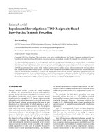
As shown in Fig. 1, the underlying music information can conceptually be represented as
layers in a pyramid (Maddage, 2005). These information layers are:
Music Structure Analysis Statistics for Popular Songs 347
T
h
Jo
u
pe
Fi
g

Ti
m
m
e
m
u
re
s
m
e
Sc
a
1) First la
y
er

2) Second la
y
notes sim

u
3) Third la
ye
instrume
n
4) Forth la
y
e
h
e p
y
ramid dia
g
u
rdain (1997)
a
rformance, liste
n

g
. 1. Information

m
e information
d
e
lod
y
contours a
n

u
sic. Melody is c
r
s
ults in harmon
y
e
chanism can eff
e
a
le chan
g
es or
m

represents the ti
m
y
er represents th
e
u
ltaneousl
y
;
e
r describes the
m
n
tal mixed vocal
(

r and above repr
e
g
ram represents

a
lso discussed
n
in
g
, understandi
g
roupin
g
in the
d
escribes the rate
n
d phrases whic
h
r
eated when a
s
y
sound. Psych
o
e
ctivel
y
distin

g
u
i
m
odulation of the

m
e information (
e
harmon
y
/mel
o
m
usic re
g
ions, i.e.

(
IMV) and silenc
e
e
sent the semant
i

music semanti
c
how sound, t
o
n

g
and ecstas
y
l
e
music structure
p
of information f
h
create music r
e
s
in
g
le note is pl
a
o
logical studies
i
sh the tones of t
h

scale in a differ
e
beats, tempo, an
d
o
d
y
which is for

m

pure vocal (PV),

e
(S);
i
cs of the popula
r
c
s which influe
n
o
ne, melod
y
,
h
e
ad to our ima
g
i
n
py
ramid
low in music. D
u
eg
ions are propo
ay
ed at a time.

P
have suggested

h
e diatonic scale
e
nt section of the

d
meter);
m
ed b
y
pla
y
in
g

m

pure instrument
r
son
g
.
n
ce our ima
g
in
h

armon
y
, comp
o
n
ation.
uratio
n
s of Har
m
o
rtional to the te
m
P
la
y
in
g
multipl
e
the human co
g
(Burred & Lerch
,

son
g
can effecti
v
m

usical
al (PI),
ations.
o
sition,
m
on
y
/
m
po of
e
notes
g
nitive
,
2004).
v
el
y
be
contours and song structures (such as repetitions of chorus verse semantic regions) are
useful for developing systems for error concealment in music streaming (Wang et al., 2003),
music protection (watermarking), music summarization (Xu et al., 2005), compression, and
music search.
Computer music research community has been developing algorithms to accurately extract
the information in music. Many of the proposed algorithms require ground truth data for
both the parameter training process and performance evaluation. For example, the
performance of a music classifier which classify the content in the music segment as vocal or
non-vocal, can be improved when the parameters of the classifier are trained with accurate

vocal and non-vocal music contents in the development dataset. Also the performance of the
classifier can effectively be measured when the evaluation dataset is accurately annotated
based on the exact music composition information. However it is difficult to create accurate
development and evaluation datasets because it is difficult to find information about the
music composition mainly due to copyright restrictions on sharing music information in the
public domain. Therefore, the current development and evaluation datasets are created by
annotating the information that is extracted using subjective listening tests. Tanghe et al.,
(2005) discussed an annotation method for drum sounds. In Goto (2006)’s method, music
scenes such as beat structure, chorus, and melody line are annotated with the help of
corresponding MIDI files. Li, et al., (2006) modified the general audio editing software so
that it becomes more convenient for identifying music semantic regions such as chorus. The
accuracy of subjective listening test hinges on subject’s hearing competence, concentration
and music knowledge. For example, it is often difficult to judge the start and end time of
vocal phrases when they are presented with strong background music. If the listener’s
concentration is disturbed, then the listening continuity is lost and then it is difficult to
accurately mark the phrase boundaries. However if we know the tempo and meter of the
music, then we can apply that knowledge to correct the errors of the phrase boundaries
which are detected in the listen tests.
Speed of music information flow is directly proportional to tempo of the music (Authors,
1949). Therefore the duration of music regions, semantic regions, inter-beat interval, and
beat positions can be measured as multiples of music notes. The proposed music
information annotation technique in this chapter, first locates the beats and onset positions
by both listening and visualizing the music signal using a graphical waveform editor. Since
the time duration of the detected beat or onset from the start of music is an integer multiple
of the duration of a smallest note, we can estimate the duration of the smallest note. Then
we carry out intensive listening exercise with the help of estimated durations of the smallest
music note to detect the time stamps of music regions and different semantic regions. Using
the annotated information, we detect the song structure and calculate the statistics of the
music information distributions.
This chapter is organized as follows. Popular music structure is discussed in section 2 and

effective information annotation procedures are explained in section 3. Section 4 details the
statistics of music information. We conclude the chapter in section 5 with a discussion.

2. Music Structure
As shown in Fig. 1, the underlying music information can conceptually be represented as
layers in a pyramid (Maddage, 2005). These information layers are:
Recent Advances in Signal Processing348
both verse and chorus are equally melodically strong. Most people can hum or sing both
chorus and verse. A Bridge links the gap between the Verse and Chorus, and may have only
two or four bars.

Fig. 4. Two examples for verse- chorus pattern repetitions.
noticed in the listening tests. Therefore, in our listening tests we detect the Middle-eighth
regions (see next section) which have a different Key from the main Key of the song.
The rhythm of words can be tailored to fit into a music phrase (Authors, 1949). The vocal
regions in music comprise of words and syllables, which are uttered according to a time
signature. Fig. 2 shows how the words “Little Jack Horner sat in the Corner” are turn into a
rhythm, and the music notation of those words. The important words or syllables in the
sentence fall onto accents to form the rhythm of the music. Typically, these words are placed
at the first beat of a bar. When TS is set to two Crotchet beats per bar, we see the duration of
the word “Little” is equal to two Quaver notes and the duration of the word “Jack” is equal
to a Crotchet note.


Fig. 2. Rhythmic flow of words

Popular song structure often contains Intro, Verse, Chorus, Bridge, Middle-eighth,
instrumental sections (INST) and Outro (Authors, 2003). As shown in Fig. 1, these parts are
built on melody-based similarity regions and content-based similarity regions. Melody-
based similarity regions are defined as the regions which have similar pitch contours

constructed from the chord patterns. Content-based similarity regions are defined as the
regions which have both similar vocal content and melody. In terms of music structure, the
Chorus sections and Verse sections in a song are considered the content-based similarity
regions and melody-based similarity regions respectively. They can be grouped to form
semantic clusters as in Fig. 3. For example, all the Chorus regions in a song form a Chorus
cluster, while all the Verse regions form a Verse cluster and so on.


Fig. 3. Semantic similarity clusters which define the structure of the popular song

A song may have an Intro of 2, 4, 8 or 16 bars long, or do not have any at all. The Intro is
usually comprised of instrumental music. Both Verse and Chorus are 8 or 16 bars long.
Typically, the Verse is not melodically as strong as the Chorus. However, in some songs
C
h
or
u
s

1
C
h
o
r
us

2
C
h
o

r
u
s

3
C
ho
r
u
s

n
C
h
o
r
u
s

i
V
er
s
e
1
V
e
r
s
e

2
V
e
r
s
e
3
V
er
s
e
n
V
e
r
s
e
k
I
n
t
r
o
O
u
t
r
o
Mi

d
d
l
e

E
i
g
h
t
h

1
Middle Eighth 2
M
i
d
d
l
e

E
i
g
h
t
h
j
B
r

i
d
g
e

1
B
r
i
d
g
e

2
B
r
i
dg
e
k
INST 1
INST 2
INST 3
INST j
Semantic clusters (regions) in
a popular song
Music Structure Analysis Statistics for Popular Songs 349
both verse and chorus are equally melodically strong. Most people can hum or sing both
chorus and verse. A Bridge links the gap between the Verse and Chorus, and may have only
two or four bars.

Fig. 4. Two examples for verse- chorus pattern repetitions.
noticed in the listening tests. Therefore, in our listening tests we detect the Middle-eighth
regions (see next section) which have a different Key from the main Key of the song.
The rhythm of words can be tailored to fit into a music phrase (Authors, 1949). The vocal
regions in music comprise of words and syllables, which are uttered according to a time
signature. Fig. 2 shows how the words “Little Jack Horner sat in the Corner” are turn into a
rhythm, and the music notation of those words. The important words or syllables in the
sentence fall onto accents to form the rhythm of the music. Typically, these words are placed
at the first beat of a bar. When TS is set to two Crotchet beats per bar, we see the duration of
the word “Little” is equal to two Quaver notes and the duration of the word “Jack” is equal
to a Crotchet note.


Fig. 2. Rhythmic flow of words

Popular song structure often contains Intro, Verse, Chorus, Bridge, Middle-eighth,
instrumental sections (INST) and Outro (Authors, 2003). As shown in Fig. 1, these parts are
built on melody-based similarity regions and content-based similarity regions. Melody-
based similarity regions are defined as the regions which have similar pitch contours
constructed from the chord patterns. Content-based similarity regions are defined as the
regions which have both similar vocal content and melody. In terms of music structure, the
Chorus sections and Verse sections in a song are considered the content-based similarity
regions and melody-based similarity regions respectively. They can be grouped to form
semantic clusters as in Fig. 3. For example, all the Chorus regions in a song form a Chorus
cluster, while all the Verse regions form a Verse cluster and so on.


Fig. 3. Semantic similarity clusters which define the structure of the popular song

A song may have an Intro of 2, 4, 8 or 16 bars long, or do not have any at all. The Intro is
usually comprised of instrumental music. Both Verse and Chorus are 8 or 16 bars long.
Typically, the Verse is not melodically as strong as the Chorus. However, in some songs
C
h
or
u
s

1
C
h
o
r
us

2
C
h
o
r
u
s

3
C
ho
r
u
s

n
C
h
o
r
u
s

i
V
er
s
e
1
V
e
r
s
e

2
V
e
r
s
e
3
V
er

s
e
n
V
e
r
s
e
k
I
n
t
r
o
O
u
t
r
o
Mi
d
d
l
e

E
i
g
h
t

h

1
Middle Eighth 2
M
i
d
d
l
e

E
i
g
h
t
h
j
B
r
i
d
g
e

1
B
r
i
d

g
e

2
B
r
i
dg
e
k
INST 1
INST 2
INST 3
INST j
Semantic clusters (regions) in
a popular song
Recent Advances in Signal Processing350

Fig. 5. Spectral and time domain visualization of (0~3657) ms long song clip from “25
Minutes” by MLTR. Quarter note length is 736.28 ms and note boundaries are highlighted
using dotted lines.

3.1. Computation of Inter-beat interval
Once the staff of a song is available, from the value of tempo and time signature we can
calculate the duration of the beat. However commercially available music albums (CDs) do
not provide staff information of the songs. Therefore subjects with a good knowledge of
theory and practice of music have to closely examine the songs to estimate the inter-beat
intervals in the song. We assume all the songs have 4/4 time signature, which is the
commonly used TS in popular songs (Goto, M. 2001, Authors, 2003). Following the results
of music composition and structure, as discussed in section 2, we only allow the positions of

beats to take place at integer multiple of smaller notes from the start point of the song.
Estimation of both inter-beat interval and song tempo using an iterative listening is
explained below, with Fig. 6 as an example.
 Play the song in audio editing software which has a GUI to visualize the time domain
signal with high resolution. While listening to the music it is noticed that there is a
steady throb to which one can clap. This duration of consecutive clapping is called
inter-beat interval. As we assume 4/4 time signature which infers that the inter-beat
interval is of quarter note length, hence four quarter notes form a bar.
 As shown in Fig. 6, the positions of both beats and note onsets can be effectively
visualized on the GUI, and j
th
position is indicated as
j
P
. By replaying the song and
zooming into the areas of neighboring beats and onset positions, we can estimate the
(0 ~ 3657)ms of the song “25 Minutes -MLTR”
Frequency (Hz)
0
2000
4000
6000
8000
10000
12000
14000
Frequency spectrum (0~15kHz) range
Time in millisecond (ms)
Time domain signal
0 500 1000 1500 2000 2500 3000 3500

-0.5
-0.3
-0.1
0
0.1
0.3
0.5
Strength
Quarter note length is 732.02 ms
Quarter note - Eighth note -
Sixteenth note -
Silence may also act as a Bridge between the Verse and Chorus of a song, but such cases are
rare. Middle-eighth, which has 4, 8 or 16 bars in length, is an alternative version of a Verse
with a new chord progression possibly modulated by a different key. Many people use the
term “Middle-eighth” and “bridge” synonymously. However, the main difference is the
middle-eighth is longer (usually 16 bars) than the bridge and usually appears after the third
verse in the song. There are instrumental sections in the song and they can be instrumental
versions of the Chorus, Verse, or entirely different tunes with a set of chords together.
Typically INST regions have 8 or 16 bars. Outro, which is the ending of the song, is usually a
fade–out of the last phrases of the chorus. We have described the parts of the song which are
commonly arranged according to the simple verse-chorus and repeat pattern. Two
variations on these themes are as follows:
(a) Intro, Verse 1, Verse 2, Chorus, Verse 3, Middle-eighth, Chorus, Chorus,
Outro
(b) Intro, Verse 1, Chorus, Verse 2, Chorus, Chorus, Outro
Fig. 4 illustrates two examples of the above two patterns. Song, “25 minutes” by MLTR
follows the pattern (a) and “Can’t Let You Go” by Mariah Carey follows the pattern (b). For
a better understanding of how artist have combined these parts to compose a song, we
conducted a survey on popular Chinese and English songs. Details of the survey are
discussed in the next section.

3. Music Structure Information Annotation
The fundamental step for audio content analysis is signal segmentation. Within a segment,
the information can be considered quasi-stationary. Feature extraction and information
modeling followed by music segmentation are the essential steps for music structure
analysis. Determination of the segment size, which is suitable for extracting certain level of
information, requires better understanding of the rate of information flow in the audio data.
Over three decades of speech processing research has revealed that 20-40 ms of fixed length
signal segmentation is appropriate for the speech content analysis (Rabiner & Juang, 2005).
The composition of music piece reveals the rate of information such as notes, chords, key,
vocal phrases, flow is proportional to inter-beat intervals.
Fig. 5 shows the quarter, eighth and sixteenth note boundaries in a song clip. It can be seen
that the fluctuation of signal properties in both spectral and time domain are aligned with
those note boundaries. Usually smaller notes, such as eighth, sixteenth and thirty-second
notes or smaller are played in the bars to align the harmony contours with the rhythm flow
of the lyrics and to fill the gap between lyrics (Authors, 1949). Therefore inter-beat
proportional music segmentation instead of fixed length segmentation has recently been
proposed for music content analysis (Maddage, 2004., Maddage, 2005., Wang, 2004).
Music Structure Analysis Statistics for Popular Songs 351

Fig. 5. Spectral and time domain visualization of (0~3657) ms long song clip from “25
Minutes” by MLTR. Quarter note length is 736.28 ms and note boundaries are highlighted
using dotted lines.

3.1. Computation of Inter-beat interval
Once the staff of a song is available, from the value of tempo and time signature we can
calculate the duration of the beat. However commercially available music albums (CDs) do
not provide staff information of the songs. Therefore subjects with a good knowledge of
theory and practice of music have to closely examine the songs to estimate the inter-beat
intervals in the song. We assume all the songs have 4/4 time signature, which is the

commonly used TS in popular songs (Goto, M. 2001, Authors, 2003). Following the results
of music composition and structure, as discussed in section 2, we only allow the positions of
beats to take place at integer multiple of smaller notes from the start point of the song.
Estimation of both inter-beat interval and song tempo using an iterative listening is
explained below, with Fig. 6 as an example.
 Play the song in audio editing software which has a GUI to visualize the time domain
signal with high resolution. While listening to the music it is noticed that there is a
steady throb to which one can clap. This duration of consecutive clapping is called
inter-beat interval. As we assume 4/4 time signature which infers that the inter-beat
interval is of quarter note length, hence four quarter notes form a bar.
 As shown in Fig. 6, the positions of both beats and note onsets can be effectively
visualized on the GUI, and j
th
position is indicated as
j
P
. By replaying the song and
zooming into the areas of neighboring beats and onset positions, we can estimate the
(0 ~ 3657)ms of the song “25 Minutes -MLTR”
Frequency (Hz)
0
2000
4000
6000
8000
10000
12000
14000
Frequency spectrum (0~15kHz) range
Time in millisecond (ms)

Time domain signal
0 500 1000 1500 2000 2500 3000 3500
-0.5
-0.3
-0.1
0
0.1
0.3
0.5
Strength
Quarter note length is 732.02 ms
Quarter note -
Eighth note -
Sixteenth note -
Silence may also act as a Bridge between the Verse and Chorus of a song, but such cases are
rare. Middle-eighth, which has 4, 8 or 16 bars in length, is an alternative version of a Verse
with a new chord progression possibly modulated by a different key. Many people use the
term “Middle-eighth” and “bridge” synonymously. However, the main difference is the
middle-eighth is longer (usually 16 bars) than the bridge and usually appears after the third
verse in the song. There are instrumental sections in the song and they can be instrumental
versions of the Chorus, Verse, or entirely different tunes with a set of chords together.
Typically INST regions have 8 or 16 bars. Outro, which is the ending of the song, is usually a
fade–out of the last phrases of the chorus. We have described the parts of the song which are
commonly arranged according to the simple verse-chorus and repeat pattern. Two
variations on these themes are as follows:
(a) Intro, Verse 1, Verse 2, Chorus, Verse 3, Middle-eighth, Chorus, Chorus,
Outro
(b) Intro, Verse 1, Chorus, Verse 2, Chorus, Chorus, Outro
Fig. 4 illustrates two examples of the above two patterns. Song, “25 minutes” by MLTR
follows the pattern (a) and “Can’t Let You Go” by Mariah Carey follows the pattern (b). For

a better understanding of how artist have combined these parts to compose a song, we
conducted a survey on popular Chinese and English songs. Details of the survey are
discussed in the next section.

3. Music Structure Information Annotation
The fundamental step for audio content analysis is signal segmentation. Within a segment,
the information can be considered quasi-stationary. Feature extraction and information
modeling followed by music segmentation are the essential steps for music structure
analysis. Determination of the segment size, which is suitable for extracting certain level of
information, requires better understanding of the rate of information flow in the audio data.
Over three decades of speech processing research has revealed that 20-40 ms of fixed length
signal segmentation is appropriate for the speech content analysis (Rabiner & Juang, 2005).
The composition of music piece reveals the rate of information such as notes, chords, key,
vocal phrases, flow is proportional to inter-beat intervals.
Fig. 5 shows the quarter, eighth and sixteenth note boundaries in a song clip. It can be seen
that the fluctuation of signal properties in both spectral and time domain are aligned with
those note boundaries. Usually smaller notes, such as eighth, sixteenth and thirty-second
notes or smaller are played in the bars to align the harmony contours with the rhythm flow
of the lyrics and to fill the gap between lyrics (Authors, 1949). Therefore inter-beat
proportional music segmentation instead of fixed length segmentation has recently been
proposed for music content analysis (Maddage, 2004., Maddage, 2005., Wang, 2004).
Recent Advances in Signal Processing352
Step 3: At beat/ onset position
j
P
, we calculate the new note length
1
j
X


as below.
1
j
j
j
P
X
NF


(4)
Step 4: Iterate the step 1 to 3 at beat or onset positions towards the end of the songs. When
these iterative steps are carried out over many of the beat and onset positions towards the
end of the song, the errors of the estimated note length are minimized. Based on the final
length estimate for the note, we can calculate the quarter note length.
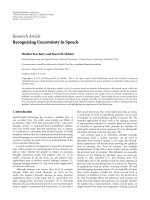
Fig. 7 shows the variation of the estimated quarter note length for two songs. Beat/onset
positions nearly divide the song into equal intervals. Beat/onset point zero (“0”) represents
the first estimation of quarter note length. The correct tempos of the songs “You are still one”
and “The woman in me” are 67 BPM and 60 BPM respectively.


Fig. 7. Variation of estimated length of the quarter note at beat/onset points when the
listening test was carried out till the end of the song.

It can be seen in the Fig. 7, that the deviation of the estimated quarter note is high at the
beginning of the song. However estimated quarter note converges to the correct value at the
second half of the song (end of the song). Reason for the fluctuation of the estimated note
length is explained below.
As shown in Fig. 6, first estimation of the note length (X
1

) is done using only audio-visual
editing software. Thus first estimation (beat/ onset point P = 0 in Fig. 7) can have very high
variation due to the prime difficulties of judging the correct boundaries of the notes. When
the song proceeds, using Eq, (1), (2), (3) and (4), we iteratively estimate the duration of the
note for the corresponding beat/onset points. Since beat/onset points near the start of the
song have shorter duration (P
j
), initial iterative estimations for the note length have higher
variation. For example in Fig. 6, beat/onset point P
1
is closer to start of the song and from
the Eq. (1) and first estimation of note length X
1
, we compute NF
1
. Eq. (2) and (3) are useful
in limiting the errors in computed NF under one frame. When X
1
is inaccurate and also P
1
is
short then the errors in computed number of frames NF
1
in Eq. (1) have higher effects in the
next estimated note length in Eq. (4). However with distant beat/onset points, i.e Pj is
longer and NF
j
is high and more accurate, then the estimated note lengths tend to converge.

Quarter note length (ms)

885
890
895
900
905
910
915
920
You are still the one - Shania twain
Beat/onset point number
1 2 3 4 5 6 7 8 9 10 11 12 13 14 15 16
0
960
970
980
990
1000
1010
1020
1030
1040
The woman in me - Shania twain
Beat/onset point number
Quarter note length (ms)
16
0
1 2 3 4 5 6 7 8 9 10 11 12 13 14 15
inter-beat interval and therefore the duration of the note
j
X

. In Fig. 6, we can see the
duration
1
X
is the first estimated eighth note.

Fig. 6. Estimation of music note

 After the first estimation, we establish a 4-step iterative listening process discussed
below to reduce the error between the estimates and the desired music note lengths.
The constraint we apply is that beat position is equal to integer multiple of frames. To
start with, first frame size is set to the estimated note, i.e. Frame size =
1
X

in Fig. 6.
Step 1
: Set the currently estimated note length as the frame size; calculate the number of
frames
j
NF
at an identified beat or onset position. For the initialization, we set 1j  .
=
j
j
j
P
NF
X
(1)

Step 2
: As the resulting
j
NF
is typically a floating point value, we measure the difference
between round up
j
NF

and
j
NF
, referred to as
D
NF
.


-
j
j
DNF NF round NF
(2)
IF
D
NF
> 0.35,
This implies, the duration of current beat or onset position
j
P

is an
integer multiple of the frames plus a half a frame. Therefore we set new
note length to the half of
j
X
. For example the new frame size is equal to
sixteenth note and if the previous frame was an eighth note. Then go to
step 1
ELSE


j j
NF round NF
(3)
Initially estimated
eighth note length
(X
1
) = 336 ms
Position P
j
Position P
j+n
X
1
Position P
1
Music Structure Analysis Statistics for Popular Songs 353
Step 3: At beat/ onset position
j

P
, we calculate the new note length
1
j
X

as below.
1
j
j
j
P
X
NF


(4)
Step 4
: Iterate the step 1 to 3 at beat or onset positions towards the end of the songs. When
these iterative steps are carried out over many of the beat and onset positions towards the
end of the song, the errors of the estimated note length are minimized. Based on the final
length estimate for the note, we can calculate the quarter note length.
Fig. 7 shows the variation of the estimated quarter note length for two songs. Beat/onset
positions nearly divide the song into equal intervals. Beat/onset point zero (“0”) represents
the first estimation of quarter note length. The correct tempos of the songs “You are still one”
and “The woman in me” are 67 BPM and 60 BPM respectively.


Fig. 7. Variation of estimated length of the quarter note at beat/onset points when the
listening test was carried out till the end of the song.

It can be seen in the Fig. 7, that the deviation of the estimated quarter note is high at the
beginning of the song. However estimated quarter note converges to the correct value at the
second half of the song (end of the song). Reason for the fluctuation of the estimated note
length is explained below.
As shown in Fig. 6, first estimation of the note length (X
1
) is done using only audio-visual
editing software. Thus first estimation (beat/ onset point P = 0 in Fig. 7) can have very high
variation due to the prime difficulties of judging the correct boundaries of the notes. When
the song proceeds, using Eq, (1), (2), (3) and (4), we iteratively estimate the duration of the
note for the corresponding beat/onset points. Since beat/onset points near the start of the
song have shorter duration (P
j
), initial iterative estimations for the note length have higher
variation. For example in Fig. 6, beat/onset point P
1
is closer to start of the song and from
the Eq. (1) and first estimation of note length X
1
, we compute NF
1
. Eq. (2) and (3) are useful
in limiting the errors in computed NF under one frame. When X
1
is inaccurate and also P
1
is
short then the errors in computed number of frames NF
1

in Eq. (1) have higher effects in the
next estimated note length in Eq. (4). However with distant beat/onset points, i.e Pj is
longer and NF
j
is high and more accurate, then the estimated note lengths tend to converge.

Quarter note length (ms)
885
890
895
900
905
910
915
920
You are still the one - Shania twain
Beat/onset point number
1 2 3 4 5 6 7 8 9 10 11 12 13 14 15 16
0
960
970
980
990
1000
1010
1020
1030
1040
The woman in me - Shania twain
Beat/onset point number

Quarter note length (ms)
16
0
1 2 3 4 5 6 7 8 9 10 11 12 13 14 15
inter-beat interval and therefore the duration of the note
j
X
. In Fig. 6, we can see the
duration
1
X
is the first estimated eighth note.

Fig. 6. Estimation of music note

 After the first estimation, we establish a 4-step iterative listening process discussed
below to reduce the error between the estimates and the desired music note lengths.
The constraint we apply is that beat position is equal to integer multiple of frames. To
start with, first frame size is set to the estimated note, i.e. Frame size =
1
X

in Fig. 6.
Step 1: Set the currently estimated note length as the frame size; calculate the number of
frames
j
NF
at an identified beat or onset position. For the initialization, we set 1j  .
=
j

j
j
P
NF
X
(1)
Step 2: As the resulting
j
NF
is typically a floating point value, we measure the difference
between round up
j
NF

and
j
NF
, referred to as
D
NF
.


-
j
j
DNF NF round NF
(2)
IF
D

NF
> 0.35,
This implies, the duration of current beat or onset position
j
P
is an
integer multiple of the frames plus a half a frame. Therefore we set new
note length to the half of
j
X
. For example the new frame size is equal to
sixteenth note and if the previous frame was an eighth note. Then go to
step 1
ELSE


j j
NF round NF
(3)
Initially estimated
eighth note length
(X
1
) = 336 ms
Position P
j
Position P
j+n
X
1

Position P
1
Recent Advances in Signal Processing354
1 to update the previously calculated region boundaries based on
new smaller note length frames.
ELSE
Minimum note resolution is considered as thirty-second note.
Therefore there is no further note length adjustment. Go to step 3.
IF (DFN < 3.5)
Then do not alter the note length. Go to step3
Step 3: Re-estimate the number of frames
( )NFvs k
and the time stamp for start position
of k
th
PV region
( )Tvs k
respectively,


( ) = round ( ) NFvs k NFvs k
(7)
( ) ( )Tvs k NFvs k X


(8)
Similar sequence of steps is followed for more accurate estimation of end time
( )Tve k
and
end frame

( )NFve k
of k
th
PV region.
Step 4: Repeat Step 1-3 for annotating the next region boundaries.
Fig. 8 shows a section of an annotated song. Thirty-second note length resolution is used for
the time stamp of music regions. Start-time and end-time of music regions found in the
initial subjective listening tests are shown under STT and EDT columns respectively.
Accurate start-frame and end-frame of the regions are shown under STF and EDF columns
respectively. According to Equation 8 accurate end-time of the instrumental Intro region (PI-
Intro) is 1263.06818182 ms (i.e. 135

93.56060606).
It can be seen in the Fig. 8 that end-time of PI has as high as 8 decimal points caused by
multiplying frame numbers with the note length which has 8 decimal places. As explained
earlier, music region boundaries can be measured as multiples of music notes. Thus it is
necessary to have a better estimation for the note-length to reduce errors at boundaries
when the number of frames for the boundary increases. Thus it becomes essential to have
more decimal places in the estimated length for the note.
3.2. Annotation of music regions
Pure vocal (PV), pure instrumental (PI), instrumental mixed vocal (IMV) and silence (S) are
the regions that can commonly be seen in a music signals (Third layer of the music structure
pyramid in Fig. 1). PV regions in the music only have signals generated from the vocal tract.
Note that the lyrics of songs would improve the music region annotation. We use lyrics text
files and employ subjects who understand the singing language to accurately stamp the
timing of the region boundaries. We obtain lyrics of the songs from the Web. Based on the
found lyrics, which are often separated into different musical phrases, we attempt to
reorganize these lyrics and further separate them into different lines based on their vocal
region continuity. Subsequently, vocal humming, for example hmm, aah, which are usually
not included in the published lyrics, is also aligned with the vocals. Common types of song

structure tagging are then used to identify a block of lyrics (e.g. Intro, Verse, Chorus, Bridge,
Middle-eighth, Outro, and Instrumental)
Based on the music knowledge explained in Fig. 2, the duration of musical phrases
can be measured by the number of musical notes. Since we have already calculated the note
length in section 3.2, we use this information to improve the listening test of time stamping
of music regions. In our annotation we assume the tempo of the song doesn’t change. Since
music signals are digitized at non-linear sampling rate (usually 44.1 kHz for CD quality), it’s
usually difficult to find the exact boundaries of vocal-instrumental regions. And also due to
the effects of subject’s concentration, hearing sensitivity and music experiences, position
markings may vary from the actual boundary positions of the region. We further propose a
4-step process to improve the time stamps of music regions.
Step 1
: Subject within his/her listening capacity marks the boundary point (start or end) of
the region. For example, let’s assume
j
P
and
j
n
P

in Fig. 6 are the start and the end time
assigned in the listening process for the k
th
pure vocal (PV) region. Let the note length be
X
.
Then we estimate the number of frames for start and end time
( )NFvs k and ( )NFve k in
Equation 5.

( ) ( )
j
j n
P P
NFvs k and NFve k
X X

 
(5)
It is empirically found that in popular songs, musical phrases are aligned with eighth or
smaller note. Therefore at the beginning of the annotation we set the note length to eighth
note.
Step 2:
As the resulting
( )NFvs k
is usually an integer multiple of note length, we further
measure the difference between
( )NFvs k and round up ( )NFvs k in order to refine the
( )NFvs k .


( ) - ( )DFN NFvs k round NFvs k
(6)
IF (0.35 < DFN < 0.5)
IF (Note length > Thirty-second note)
Reduce the note length to next smaller one (e.g. Eighth to
Sixteenth or Sixteenth to thirty-second note levels) and go to step
Music Structure Analysis Statistics for Popular Songs 355
1 to update the previously calculated region boundaries based on
new smaller note length frames.

ELSE
Minimum note resolution is considered as thirty-second note.
Therefore there is no further note length adjustment. Go to step 3.
IF (DFN < 3.5)
Then do not alter the note length. Go to step3
Step 3
: Re-estimate the number of frames
( )NFvs k
and the time stamp for start position
of k
th
PV region
( )Tvs k
respectively,


( ) = round ( ) NFvs k NFvs k
(7)
( ) ( )Tvs k NFvs k X


(8)
Similar sequence of steps is followed for more accurate estimation of end time
( )Tve k
and
end frame
( )NFve k
of k
th
PV region.

Step 4
: Repeat Step 1-3 for annotating the next region boundaries.
Fig. 8 shows a section of an annotated song. Thirty-second note length resolution is used for
the time stamp of music regions. Start-time and end-time of music regions found in the
initial subjective listening tests are shown under STT and EDT columns respectively.
Accurate start-frame and end-frame of the regions are shown under STF and EDF columns
respectively. According to Equation 8 accurate end-time of the instrumental Intro region (PI-
Intro) is 1263.06818182 ms (i.e. 135

93.56060606).
It can be seen in the Fig. 8 that end-time of PI has as high as 8 decimal points caused by
multiplying frame numbers with the note length which has 8 decimal places. As explained
earlier, music region boundaries can be measured as multiples of music notes. Thus it is
necessary to have a better estimation for the note-length to reduce errors at boundaries
when the number of frames for the boundary increases. Thus it becomes essential to have
more decimal places in the estimated length for the note.
3.2. Annotation of music regions
Pure vocal (PV), pure instrumental (PI), instrumental mixed vocal (IMV) and silence (S) are
the regions that can commonly be seen in a music signals (Third layer of the music structure
pyramid in Fig. 1). PV regions in the music only have signals generated from the vocal tract.
Note that the lyrics of songs would improve the music region annotation. We use lyrics text
files and employ subjects who understand the singing language to accurately stamp the
timing of the region boundaries. We obtain lyrics of the songs from the Web. Based on the
found lyrics, which are often separated into different musical phrases, we attempt to
reorganize these lyrics and further separate them into different lines based on their vocal
region continuity. Subsequently, vocal humming, for example hmm, aah, which are usually
not included in the published lyrics, is also aligned with the vocals. Common types of song
structure tagging are then used to identify a block of lyrics (e.g. Intro, Verse, Chorus, Bridge,
Middle-eighth, Outro, and Instrumental)
Based on the music knowledge explained in Fig. 2, the duration of musical phrases

can be measured by the number of musical notes. Since we have already calculated the note
length in section 3.2, we use this information to improve the listening test of time stamping
of music regions. In our annotation we assume the tempo of the song doesn’t change. Since
music signals are digitized at non-linear sampling rate (usually 44.1 kHz for CD quality), it’s
usually difficult to find the exact boundaries of vocal-instrumental regions. And also due to
the effects of subject’s concentration, hearing sensitivity and music experiences, position
markings may vary from the actual boundary positions of the region. We further propose a
4-step process to improve the time stamps of music regions.
Step 1: Subject within his/her listening capacity marks the boundary point (start or end) of
the region. For example, let’s assume
j
P
and
j
n
P

in Fig. 6 are the start and the end time
assigned in the listening process for the k
th
pure vocal (PV) region. Let the note length be
X
.
Then we estimate the number of frames for start and end time
( )NFvs k and ( )NFve k in
Equation 5.
( ) ( )
j
j n
P P

NFvs k and NFve k
X X

 
(5)
It is empirically found that in popular songs, musical phrases are aligned with eighth or
smaller note. Therefore at the beginning of the annotation we set the note length to eighth
note.
Step 2: As the resulting
( )NFvs k
is usually an integer multiple of note length, we further
measure the difference between
( )NFvs k and round up ( )NFvs k in order to refine the
( )NFvs k .


( ) - ( )DFN NFvs k round NFvs k
(6)
IF (0.35 < DFN < 0.5)
IF (Note length > Thirty-second note)
Reduce the note length to next smaller one (e.g. Eighth to
Sixteenth or Sixteenth to thirty-second note levels) and go to step
Recent Advances in Signal Processing356

Fig. 9. Visualization of the components in a popular song.

4. Statistical Analysis of the Music Information
We conduct statistical analysis over a database of 420 songs, 120 English songs and 100
songs of each Chinese, Indonesian and German languages. Table 1 summarizes the database.
We then carry out listening tests to extract the structural information. An average of 3 hours

of intensive listening is required all the annotations per song. The following subsections
pictorially discuss the statistics.

4.1. Time information statistics
Tempo describes the speed of the information flow in the music. Fig. 10-(a) discusses the
average (Avg) and standard deviation (Std) of tempos based on gender male/ female and
total for different languages. Avg and Std of all the songs (i.e. 420 songs) are shown in Fig.
10-(b). The standard deviation (Std) of tempos, in other words the fluctuation of the tempos
tells us how dynamic the songs in that cluster are.
It can be seen in Fig. 10-(a) that for all the languages, Avg and Std of the tempos in the male
song cluster are higher than they are in the female song cluster. In our song collection,
Indonesian male songs have the highest Avg tempo with respect to other languages. As
shown in Fig. 10-(b), Avg tempo of male songs is 15 BPM higher than the Avg tempo of
female songs and Std of female songs is 5 BPM lower than that of male songs. Fig. 11 details
the tempo statistics in histograms.


Fig. 10. Tempo statistics of the songs
Song structure
Middle Eight
MP-1 Vocal instrum ental
MP-r Vocal instrumental
MP-n
me
Vocal instrumental
Bridge
OR/AND
MP(s)
OR/AND
MP(s)

MP-1 Vocal instrum ental
MP-r Vocal instrum ental
MP-n
b
Vocal instrum ental
InstrumentalVocal
Vocal (Humming) Instrumental
MP(s)
InstrumentalVocal
Outro
Chorus fade out
OR/AND
MP- music phrase
MP(s)
InstrumentalVocal
Intro
MP(s)
MP(s)
OR/AND
OR/AND
Vocal Instrumental
Vocal (Humming)
Instrumental
INST
MP-1 Vocal instrum ental
MP-r Vocal instrum ental
MP-n
I
Vocal instrum ental
Chorus

MP-1 Vocal instrumental
MP-r Vocal instrum ental
MP-n
c
Vocal instrumental
Verse
MP-1 Vocal instrumental
MP-r Vocal instrumental
MP-n
v
Vocal instrumental
100.26
100.002
118.18
97.58
3
5
.
5
3
3
1
.
1
8
3
8
.
7
8

3
3
.
8
5
91.19
86.37
84.63
94.12
2
9
.
9
7
2
7
.
6
9
2
4
.
9
2
3
3
.
7
3
88.78

89.38
100.13
107.89
2
8
.
8
1
2
9
.
8
8
3
3
.
2
6
3
7
.
6
7
20
30
40
50
60
70
80

90
100
110
120
Avg Std Avg Std Avg Std
Male Female Total
Indonesian
Chinese
English
German
Tempo (beats per minutes -BPM)
(a)
(b)
20
30
40
50
60
70
80
90
100
110
104.01
89.08
96.54
3
4.
8
4

2
9
.
0
8
3
3
.
4
3
Avg Std
Male
Female
All Song

Fig. 8. Section of manually annotated vocal and instrumental boundaries of the first few
phrases of the song “The Actor” by MLTR. The frame length is equal to the thirty-second
note (93.56060606 ms).

3.3. Annotation of song structure
We follow these assumptions while annotating the semantic regions in a popular song.
 Verse and Choruses are usually 8 or 16 bars, but can be 4 bars.
 All the Verses only share similar melody but different vocals.
 All the Choruses have similar vocals and melody.
 The melody of the Verse and Chorus can be similar or different.
 The bridge is less than 8 bars and can be instrumental
 The Middle-eighth is usually 8 or 16 bars and has a different key from the original
song. Middle-eighth regions are identified by detecting the region(s) which have a
different key from the main key in the intensive listening test.
 INST is usually 8 or 16 bar long instrumental section which appears neither begin

nor the end of the song.
Fig. 9 explains the general overview of the components of the song structure. Usually Verse,
Chorus and Middle-eighth start with vocals and may end with either vocals or instrumental
section. In Fig. 8, we have shown the annotation of the Intro, Verse 1, and Chorus 1, and the
start of the Verse 2. We set the tolerance of ± 2 bars for judging the duration of Verse or
Chorus.
*STT and EDT are found in the listening test. STF and EDF are computed in the annotation process
Music Structure Analysis Statistics for Popular Songs 357

Fig. 9. Visualization of the components in a popular song.

4. Statistical Analysis of the Music Information
We conduct statistical analysis over a database of 420 songs, 120 English songs and 100
songs of each Chinese, Indonesian and German languages. Table 1 summarizes the database.
We then carry out listening tests to extract the structural information. An average of 3 hours
of intensive listening is required all the annotations per song. The following subsections
pictorially discuss the statistics.

4.1. Time information statistics
Tempo describes the speed of the information flow in the music. Fig. 10-(a) discusses the
average (Avg) and standard deviation (Std) of tempos based on gender male/ female and
total for different languages. Avg and Std of all the songs (i.e. 420 songs) are shown in Fig.
10-(b). The standard deviation (Std) of tempos, in other words the fluctuation of the tempos
tells us how dynamic the songs in that cluster are.
It can be seen in Fig. 10-(a) that for all the languages, Avg and Std of the tempos in the male
song cluster are higher than they are in the female song cluster. In our song collection,
Indonesian male songs have the highest Avg tempo with respect to other languages. As
shown in Fig. 10-(b), Avg tempo of male songs is 15 BPM higher than the Avg tempo of
female songs and Std of female songs is 5 BPM lower than that of male songs. Fig. 11 details
the tempo statistics in histograms.

Fig. 10. Tempo statistics of the songs
Song structure
Middle Eight
MP-1 Vocal instrum ental
MP-r Vocal instrumental
MP-n
me
Vocal instrumental
Bridge
OR/AND
MP(s)
OR/AND
MP(s)
MP-1 Vocal instrum ental
MP-r Vocal instrum ental
MP-n
b
Vocal instrum ental
InstrumentalVocal
Vocal (Humming) Instrumental
MP(s)
InstrumentalVocal
Outro
Chorus fade out
OR/AND
MP- music phrase
MP(s)
InstrumentalVocal

Intro
MP(s)
MP(s)
OR/AND
OR/AND
Vocal Instrumental
Vocal (Humming)
Instrumental
INST
MP-1 Vocal instrum ental
MP-r Vocal instrumental
MP-n
I
Vocal instrum ental
Chorus
MP-1 Vocal instrumental
MP-r Vocal instrumental
MP-n
c
Vocal instrumental
Verse
MP-1 Vocal instrumental
MP-r Vocal instrumental
MP-n
v
Vocal instrumental
100.26
100.002
118.18
97.58

3
5
.
5
3
3
1
.
1
8
3
8
.
7
8
3
3
.
8
5
91.19
86.37
84.63
94.12
2
9
.
9
7
2

7
.
6
9
2
4
.
9
2
3
3
.
7
3
88.78
89.38
100.13
107.89
2
8
.
8
1
2
9
.
8
8
3
3

.
2
6
3
7
.
6
7
20
30
40
50
60
70
80
90
100
110
120
Avg Std Avg Std Avg Std
Male Female Total
Indonesian
Chinese
English
German
Tempo (beats per minutes -BPM)
(a)
(b)
20
30

40
50
60
70
80
90
100
110
104.01
89.08
96.54
3
4.
8
4
2
9
.
0
8
3
3
.
4
3
Avg Std
Male
Female
All Song

Fig. 8. Section of manually annotated vocal and instrumental boundaries of the first few
phrases of the song “The Actor” by MLTR. The frame length is equal to the thirty-second
note (93.56060606 ms).

3.3. Annotation of song structure
We follow these assumptions while annotating the semantic regions in a popular song.
 Verse and Choruses are usually 8 or 16 bars, but can be 4 bars.
 All the Verses only share similar melody but different vocals.
 All the Choruses have similar vocals and melody.
 The melody of the Verse and Chorus can be similar or different.
 The bridge is less than 8 bars and can be instrumental
 The Middle-eighth is usually 8 or 16 bars and has a different key from the original
song. Middle-eighth regions are identified by detecting the region(s) which have a
different key from the main key in the intensive listening test.
 INST is usually 8 or 16 bar long instrumental section which appears neither begin
nor the end of the song.
Fig. 9 explains the general overview of the components of the song structure. Usually Verse,
Chorus and Middle-eighth start with vocals and may end with either vocals or instrumental
section. In Fig. 8, we have shown the annotation of the Intro, Verse 1, and Chorus 1, and the
start of the Verse 2. We set the tolerance of ± 2 bars for judging the duration of Verse or
Chorus.
*STT and EDT are found in the listening test. STF and EDF are computed in the annotation process
Recent Advances in Signal Processing358

Fig. 13. Histograms of region content distributions

4.3. Song structure statistics
General knowledge about popular song structures is explained in section 2.4. In this section,
important statistics about the components of the song structures are explained in point 1 to 9.
Point 10 and 11 discuss the statistics of popular song structures. The song structure statistics

are calculated using English, Chinese and Indonesian songs.

0
1
2
3
4
5
6
7
8
9
10
0
2
4
6
8
10
12
0 10 20 30 40 50 60 70 80 90 100
0 10 20 30 40 50 60 70 80 90 100
0
2
4
6
8
10
12
0 10 20 30 40 50 60 70 80 90 100

0
2
4
6
8
10
12
0 10 20 30 40 50 60 70 80 90 100
0
2
4
6
8
10
12
14
0 10 20 30 40 50 60 70 80 90 100
0
2
4
6
8
10
12
0 10 20 30 40 50 60 70 80 90 100
0
5
10
15
20

25
30
35
0 2 4 6 8 10 12 14 16 18 20
0
5
10
15
20
25
30
35
40
45
0 2 4 6 8 10 12 14 16 18 20
0 2 4 6 8 10 12 14 16 18 20
0
2
4
6
8
10
12
14
16
18
0
2
4
6

8
10
12
0 10 20 30 40 50 60 70 80 90 100
0
2
4
6
8
10
12
0 10 20 30 40 50 60 70 80 90 100
0
5
10
15
20
25
30
35
40
45
50
0 2 4 6 8 10 12 14 16 18 20
0
10
20
30
40
50

60
70
0 2 4 6 8 10 12 14 16 18 20
0
2
4
6
8
10
12
14
16
18
20
0 10 20 30 40 50 60 70 80 90 100
0
2
4
6
8
10
12
14
0 10 20 30 40 50 60 70 80 90 100
Number of songs
Number of songs
Number of songs
Number of songs
Number of songs
Percentages of region contents in a song Percentages of region contents in a song Percentages of region contents in a song

S regions for all
songs
PI regions for all
the songs
IMV regions for
all the songs
S regions for
German songs
PI regions for
German songs
IMV regions for
German songs
IMV regions for
Indonesian songs
PI regions for
Indonesian songs
S regions for
Indonesian songs
S regions for
Chinese songs
S regions for
English songs
PI regions for
Chinese songs
PI regions for
English songs
IMV regions for
Chinese songs
IMV regions for
English songs

Fig. 11. Tempo statistic histograms

4.2. Music region statistics
Equation (9) describes the distribution of content with respect to region types for songs in
the test database. We have
1,2,3,4k

to represent PV, PI, IMV or S regions respectively.
Let
( )
N
F k be the total number of frames belonging to region type k and
all
NF
be the
total number of frames in a song or a collection of songs. We have
( )
k
all
NF k
D
NF

(9)
Fig. 12 shows the average content distribution
k
D
in our database. According to Fig. 12-(a),
pure vocal regions in popular music are rare. Silence regions mostly appear at the

beginning and at the ending of a song, and constitute a small percentage in the distribution
as well. Fig. 12-(b) explains the content distributions by genders and languages. The
deviation of IMV and PV region contents is around 10% across the genders and languages.
However the deviation is around 2% per song for silence regions. Fig. 13 explains the region
content distributions in histograms.


Fig. 12. Distribution of region contents over 420 songs

All songs
0
50
100 150 200 250
2
4
6
8
10
12
14
16
18
20
0 50
100 150 200 250
2
4
6
8
10

12
14
16
18
20
English
0
50
100 150 200 250
Chinese
2
4
6
8
10
12
14
16
18
20
Indonesian
2
4
6
8
10
12
14
16
18

20
0 50
100 150 200 250
German
2
4
6
8
10
12
14
16
18
20
0 50
100 150 200 250
Female
0
50
100 150 200 250
2
4
6
8
10
12
14
16
18
20

Male
0
50
100 150 200 250
2
4
6
8
10
12
14
16
18
20
Beats per minutes
(BPMs) number
Number of values
per BPM number
0
1
2
3
20
30
40
50
60
70
80
M

a
l
e
F
e
m
a
l
e
T
o
t
a
l
M
a
l
e
F
e
m
a
l
e
T
o
t
a
l
M

a
l
e
F
e
m
a
l
e
T
o
t
a
l
M
a
l
e
F
e
m
a
l
e
T
o
t
a
l
English Chinese Indonesian German

IMV
PV
PI
S
62.46
0
.1
7
35.48
1.87
IMV PV PI S
0
10
20
30
40
50
60
70
Percentage (%) of region contents in a song
(a) (b)
Music Structure Analysis Statistics for Popular Songs 359

Fig. 13. Histograms of region content distributions

4.3. Song structure statistics
General knowledge about popular song structures is explained in section 2.4. In this section,
important statistics about the components of the song structures are explained in point 1 to 9.
Point 10 and 11 discuss the statistics of popular song structures. The song structure statistics
are calculated using English, Chinese and Indonesian songs.

0
1
2
3
4
5
6
7
8
9
10
0
2
4
6
8
10
12
0 10 20 30 40 50 60 70 80 90 100
0 10 20 30 40 50 60 70 80 90 100
0
2
4
6
8
10
12
0 10 20 30 40 50 60 70 80 90 100
0

2
4
6
8
10
12
0 10 20 30 40 50 60 70 80 90 100
0
2
4
6
8
10
12
14
0 10 20 30 40 50 60 70 80 90 100
0
2
4
6
8
10
12
0 10 20 30 40 50 60 70 80 90 100
0
5
10
15
20
25

30
35
0 2 4 6 8 10 12 14 16 18 20
0
5
10
15
20
25
30
35
40
45
0 2 4 6 8 10 12 14 16 18 20
0 2 4 6 8 10 12 14 16 18 20
0
2
4
6
8
10
12
14
16
18
0
2
4
6
8

10
12
0 10 20 30 40 50 60 70 80 90 100
0
2
4
6
8
10
12
0 10 20 30 40 50 60 70 80 90 100
0
5
10
15
20
25
30
35
40
45
50
0 2 4 6 8 10 12 14 16 18 20
0
10
20
30
40
50
60

70
0 2 4 6 8 10 12 14 16 18 20
0
2
4
6
8
10
12
14
16
18
20
0 10 20 30 40 50 60 70 80 90 100
0
2
4
6
8
10
12
14
0 10 20 30 40 50 60 70 80 90 100
Number of songs
Number of songs
Number of songs
Number of songs
Number of songs
Percentages of region contents in a song Percentages of region contents in a song Percentages of region contents in a song
S regions for all

songs
PI regions for all
the songs
IMV regions for
all the songs
S regions for
German songs
PI regions for
German songs
IMV regions for
German songs
IMV regions for
Indonesian songs
PI regions for
Indonesian songs
S regions for
Indonesian songs
S regions for
Chinese songs
S regions for
English songs
PI regions for
Chinese songs
PI regions for
English songs
IMV regions for
Chinese songs
IMV regions for
English songs

Fig. 11. Tempo statistic histograms

4.2. Music region statistics
Equation (9) describes the distribution of content with respect to region types for songs in
the test database. We have
1,2,3,4k

to represent PV, PI, IMV or S regions respectively.
Let
( )
N
F k be the total number of frames belonging to region type k and
all
NF
be the
total number of frames in a song or a collection of songs. We have
( )
k
all
NF k
D
NF

(9)
Fig. 12 shows the average content distribution
k
D
in our database. According to Fig. 12-(a),
pure vocal regions in popular music are rare. Silence regions mostly appear at the
beginning and at the ending of a song, and constitute a small percentage in the distribution

as well. Fig. 12-(b) explains the content distributions by genders and languages. The
deviation of IMV and PV region contents is around 10% across the genders and languages.
However the deviation is around 2% per song for silence regions. Fig. 13 explains the region
content distributions in histograms.


Fig. 12. Distribution of region contents over 420 songs

All songs
0
50
100 150 200 250
2
4
6
8
10
12
14
16
18
20
0 50
100 150 200 250
2
4
6
8
10
12

14
16
18
20
English
0
50
100 150 200 250
Chinese
2
4
6
8
10
12
14
16
18
20
Indonesian
2
4
6
8
10
12
14
16
18
20

0 50
100 150 200 250
German
2
4
6
8
10
12
14
16
18
20
0 50
100 150 200 250
Female
0
50
100 150 200 250
2
4
6
8
10
12
14
16
18
20
Male

0
50
100 150 200 250
2
4
6
8
10
12
14
16
18
20
Beats per minutes
(BPMs) number
Number of values
per BPM number
0
1
2
3
20
30
40
50
60
70
80
M
a

l
e
F
e
m
a
l
e
T
o
t
a
l
M
a
l
e
F
e
m
a
l
e
T
o
t
a
l
M
a

l
e
F
e
m
a
l
e
T
o
t
a
l
M
a
l
e
F
e
m
a
l
e
T
o
t
a
l
English Chinese Indonesian German
IMV

PV
PI
S
62.46
0
.1
7
35.48
1.87
IMV PV PI S
0
10
20
30
40
50
60
70
Percentage (%) of region contents in a song
(a) (b)
Recent Advances in Signal Processing360




4.4. Summary of song structure statistics
 It is found that over 95% of the English, Chinese and Indonesian songs have an
introduction (i.e. Intro) and over 65% of them have instrumental Intros.
 Over 90% of songs have either instrumental mixed vocals or an instrumental
Outro. Around 38% of English songs have fading Choruses (vocal + melody) as

Outro.
1 2 3 4 5 6 7 8
1
2.50
2
0.83 7.50 35.83 18.33 1.67
3
1.67 6.67 9.17 4.17 0.83
4
0.83 2.50 5.00 0.83
5
0.83
6
0.83
7
8
Number of Verses
Number of choruses
English songs
1 2 3 4 5 6 7 8
1
5.00
4.00 1.00
2
13.00 18.00 8.00 2.00
1.00
3
8.00 18.00 5.00 1.00
1.00
4

4.00 5.00
1.00
5
1.00
3.00
6
7
8
0
1.00
Number of Verses
Number of choruses
Chinese songs
(8) Percentage of songs have verse - chorus combinations
1 2 3 4 5 6 7 8
1
1.00
1.00
2
1.00 6.00 15.00 7.00 1.00
1.00
3
11.00 25.00 10.00 1.00
3.00
4
3.00 4.00 6.00
1.00
5
2.00
6

7
8
0
1.00
Number of Verses
Number of choruses
Indonesian Songs
1 2 3 4 5 6 7 8
1
2.81
1.56 0.31
2
0.63 8.75 23.75 11.56 1.56
0.31 0.31
3
0.63 8.44 16.88 6.25 0.94
1.25
4
0.31 3.13 4.69 2.19
0.63
5
1.25
0.94
6
0.31
7
8
0
0.31
0.31

Number of Verses
Number of choruses
All the Songs
(9) length of verse and chorus
Song structures
(10)
(11)



English Chinese Indonesian
INST-0
48.33% 18.00% 35.00%
INST-1
42.50% 65.00% 51.00%
INST-2
9.17% 17.00% 12.00%
All Songs
34.69%
52.19%
12.50%
INST-3
2.00% 0.63%
(7) Percentages of songs that have number of verses (n-V) and number of choruses (n-C)
English
Chinese
Indonesian
All Songs
Number of verse (V) and Chorus (c) regions
0

-
V
1
-
V
2
-
V
3
-
V
4
-
V
5
-
V
6
-
V
7
-
V
8
-
V
0
-
C
1

-
C
2
-
C
3
-
C
4
-
C
5
-
C
6
-
C
7
-
C
8
-
C
Percentage of songs
0
10
20
30
40
50

60
70
Verse Chorus Verse Chorus Verse Chorus Verse
0
1.00 1.00
1
2.50 3.33 10.00 2.00 1.00 4.06
2
64.17 20.00 41.00 30.00 32.00 23.00 37.50
3
22.50 50.00 33.00 48.00 50.00 45.00 28.75
4
9.17 23.33 11.00 13.00 14.00 23.00 22.50
5
0.83 2.50 4.00 5.00 2.00 3.00 5.94
6
0.83 0.83 1.00 3.00 0.94
7
1.00
Chorus
0.63
1.56
24.06
47.81
20.00
3.44
1.56
0.31
8
1.00 0.31

English Chinese Indonesian
All songs
No of
regions
Music Structure Analysis Statistics for Popular Songs 361




4.4. Summary of song structure statistics
 It is found that over 95% of the English, Chinese and Indonesian songs have an
introduction (i.e. Intro) and over 65% of them have instrumental Intros.
 Over 90% of songs have either instrumental mixed vocals or an instrumental
Outro. Around 38% of English songs have fading Choruses (vocal + melody) as
Outro.
1 2 3 4 5 6 7 8
1
2.50
2
0.83 7.50 35.83 18.33 1.67
3
1.67 6.67 9.17 4.17 0.83
4
0.83 2.50 5.00 0.83
5
0.83
6
0.83
7
8

Number of Verses
Number of choruses
English songs
1 2 3 4 5 6 7 8
1
5.00
4.00 1.00
2
13.00 18.00 8.00 2.00
1.00
3
8.00 18.00 5.00 1.00
1.00
4
4.00 5.00
1.00
5
1.00
3.00
6
7
8
0
1.00
Number of Verses
Number of choruses
Chinese songs
(8) Percentage of songs have verse - chorus combinations
1 2 3 4 5 6 7 8
1

1.00
1.00
2
1.00 6.00 15.00 7.00 1.00
1.00
3
11.00 25.00 10.00 1.00
3.00
4
3.00 4.00 6.00
1.00
5
2.00
6
7
8
0
1.00
Number of Verses
Number of choruses
Indonesian Songs
1 2 3 4 5 6 7 8
1
2.81
1.56 0.31
2
0.63 8.75 23.75 11.56 1.56
0.31 0.31
3
0.63 8.44 16.88 6.25 0.94

1.25
4
0.31 3.13 4.69 2.19
0.63
5
1.25
0.94
6
0.31
7
8
0
0.31
0.31
Number of Verses
Number of choruses
All the Songs
(9) length of verse and chorus
Song structures
(10)
(11)



English Chinese Indonesian
INST-0
48.33% 18.00% 35.00%
INST-1
42.50% 65.00% 51.00%
INST-2

9.17% 17.00% 12.00%
All Songs
34.69%
52.19%
12.50%
INST-3
2.00% 0.63%
(7) Percentages of songs that have number of verses (n-V) and number of choruses (n-C)
English
Chinese
Indonesian
All Songs
Number of verse (V) and Chorus (c) regions
0
-
V
1
-
V
2
-
V
3
-
V
4
-
V
5
-

V
6
-
V
7
-
V
8
-
V
0
-
C
1
-
C
2
-
C
3
-
C
4
-
C
5
-
C
6
-

C
7
-
C
8
-
C
Percentage of songs
0
10
20
30
40
50
60
70
Verse Chorus Verse Chorus Verse Chorus Verse
0
1.00 1.00
1
2.50 3.33 10.00 2.00 1.00 4.06
2
64.17 20.00 41.00 30.00 32.00 23.00 37.50
3
22.50 50.00 33.00 48.00 50.00 45.00 28.75
4
9.17 23.33 11.00 13.00 14.00 23.00 22.50
5
0.83 2.50 4.00 5.00 2.00 3.00 5.94
6

0.83 0.83 1.00 3.00 0.94
7
1.00
Chorus
0.63
1.56
24.06
47.81
20.00
3.44
1.56
0.31
8
1.00 0.31
English Chinese Indonesian
All songs
No of
regions