Recent Advances in Signal Processing 2011 Part 13 pot

Bạn đang xem bản rút gọn của tài liệu. Xem và tải ngay bản đầy đủ của tài liệu tại đây (2.89 MB, 35 trang )

On the role of receiving beamforming in transmitter cooperative communications 407

scenario in the previous section. Although only the case with one interfering cluster is
modelled, the extension to several clusters is straightforward and will reinforce the
Gaussian hypothesis for the interference that we will claim. The received signal i
1
at sensor 1
(our reference) in the original cluster coming from the interfering one is:
intint11
xFm
H
MIMO
Pi



(36)
Where m
1
is the flat fading channel from interfering cluster to the reference sensor, F
int
(also
assumed power normalized) is the precoding performed at that cluster and x
int
is the
transmitted sequence.
)1,0(

means the extra loss compared to the desired link to
represent the fact that the interfering cluster may be further away (according to Figure 1,


=1). The mean interference power clearly becomes:

MIMO
H
MIMO
PPP
H

1intint1int
mFFm
(37)
Central Limit Theorem confirms the Gaussian hypothesis as a linear combination of i.i.d.
random variables. So, the equivalent effect of interference makes effective noise to be
increased from:

MIMOeff
P
22

(38)
Clearly, the SNR becomes negative if we consider the circular distributions of sensors in
figure 4 and in any case, the throughput degrades very significantly. Fig. 6 shows this
performance degradation compared to the no interference case, in a 4x4 system (4 transmit
sensors, 4 receive sensors). Recalling that the interference is modelled as an additional
AWGN contribution, the sum rate of the system is depicted for different Gains G already
described and for different values of the noise variance,

eff
2
.

0 5 10 15 20 25 30
2
4
6
8
10
12
14
16
18
20
22
Gain [dB]
Sum rate [b/s/Hz]
System 4x4

2
eff
=0.3

2
eff
=0.03

Fig. 6. Performance degradation due to interference

This previous result states that independently of the cooperation strategy, wireless ad hoc
networks need some kind of coordination between neighbouring clusters in terms of
multiple access strategy to avoid this large performance degradation.

 
 
nFxH
Fxh
Fxh
Fxh
y
~
~
1
~
1
~
1
1
2
22
2
11
1




























ss
N
H
N
r
rMIMO
H
r
rMIMO
H
n
GP
GPP

n
GP
GPP
n





(33)
Now H
1
collects all the effects related to the virtual MIMO creation and n
~
is the equivalent
white normalized Gaussian noise. It is remarkable that this situation becomes a standard
MIMO problem (as in equation (1)) but with non identical distributions of the matrix entries.
Sum rate of this problem denoted as R
Coop
using the dual BC-MAC decomposition is
MIMO
N
k
k
N
k
kk
H
k
N

k
kCoop
Ptr
RR
s
ss














1
11
todConstraine
detlog
Q
HQHI

(34)
where matrices Q
k

represent the autocorrelation matrices in the dual MAC problem. As this
optimization problem in fact depends on the choice of P
t
and P
r
, the solution may be
expressed as follows:

















2
,
1logmax

GP
NRR

t
sCoop
PP
Sum
rt

(35)
that must be solved by exhaustive search in P
r
and P
t
. Fig. 5 shows the schematic equivalent
view of the simplest case where 2 transmit sensors and 2 receiving sensors are allowed to
cooperate. It is observed that the original interference channel is transformed into a BC
channel with multiple receiving antennas. This is the reason of the performance
improvement.
Tx
Rx

Tx
Rx

Fig. 5. Left hand side, original scenario. Right hand side, equivalent scenario with Tx /Rx
cooperation

3.2 Scenario with intercluster interference
The model presented in this section permits us to quantify the new situation where another
cluster is also transmitting and therefore causing interference to the aforementioned
Recent Advances in Signal Processing408

The key issue now is how to design the beamfoming to improve performance. Our proposal
follows a double purpose: on the one hand, eliminate intercluster interference, and on the
other maximize the intracluster throughput. In order to provide a reasonable model for this
situation, we recall again the suboptimal approach described in section 1.

3.3 Proposed solution for the interference scenario
Fig.1 also shows the block diagram of the proposed scheme where H
k
(N
b
, N
s
) represents the
equivalent channel to the subcluster forming the beamforming. We will force N
b
>N
s
for rank
reasons as we will describe later. r
k
represents again the beamforming to be designed.
In the interference-free scenario, the beamforming design would be the same as that
described in section 2. However, current criteria assume that the interference channels are
known at the receiver beamformers location. The suboptimal procedure can be described in
several key ideas:
First point: eliminate completely the intercluster interference. In order to guarantee this
condition, every beamformer must fulfil r
k
:
0

intint
xFMr
k
H
k

(39)
where M
k
is the channel (Ns, N
b
) between the interfering cluster and the beamformer k.
Equation (39) is quite simple under the rank condition already mentioned because r
k
must
belong to the null space of M
k
.
Second point: recalling (9) a suboptimal solution to this problem is proposed in the real
multiantenna scenario without interference. We showed that the beamformers maximizing
throughput must be found from the following eigenanalysis (we show this again for
convenience).
kk
H
kk
rrHH
max


(40)

Third point: in order to fulfil both previous points, our solution is based on the
decomposition of
k
H into 2 orthogonal components, one of them expanding the null
subspace of M
k
.
kk
kk
k
MM
HHH


(41)
The final solution modifies the criteria given by (9) as


kk
H
kk
kk
rrHH
MM
max




(42)

3.4 Simulation Results
This section addresses some of the most remarkable results. The first scenario that is
considered assumes a very closely spaced transmit sensor group, as well as the receive
group, modelled with a high gain value (G=1000, that is, 30dB). The AWGN variance at the
receive sensors is set to a very low value, in order to notice the degradation due to the
intercluster interference and not to start with the scenario that is already close to saturation.
Therefore, the noise variance is set to 0.03. A two transmit and two receive sensors (2x2)
system is considered, with a variable number of dummy sensors – from 2 to 6 (that is, 3 to 7
cooperative sensors) and the simulation results are shown in Figure 9.

In order to provide a feasible solution for this problem, we recall that in fact in a cluster are
usually located many sensors additional to the already mentioned N
s
that use to be sleeping
until some event wakes them. The idea that we propose is to awake a set of sensors N
b
-1 per
every N
s
sensors so involving N
b
N
s
sensors where in each group of N
b
sensors, the N
b
-1
sensors play the role of dumb antennas in an irregular bidimensional beamforming. This

way, instead of Rx cooperation in terms of a throughput increase following the BC approach
showed in Fig. 4, we exploit the SDMA (Space Division Multiple Access) principles.
Although this is a well know topic in the literature, we have to claim that decentralized
beamforming adds some new features that must be looked at carefully. In fact we are
dealing with irregular spatially distributed beamformers (Ochiai et al, 2005;Mudumbai et al,
2007; Barton et al, 2007) where preliminary results point out a significant array gain. It is
also important to remark that the main drawback of this approach is that synchronization
must be quite accurate. In particular, (Ochiai et al, 2005) analysed this case from the point of
view of spatially random sampling and it shows the significant average gain (now
beamforming performance becomes a random variable) and an acceptable average side
lobes level.
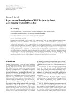
The use of dummy sensors and the equivalent MIMO system are shown in Fig. 7 and Fig. 8.
The 2x2 system with 3 dummy sensors per each receive sensor is depicted. It can be seen
that the equivalent system becomes a MIMO system with a single transmitter with N
t
=2
antennas, and N
s
=2 receivers with N
b
(4) antennas. The equivalent MIMO fading channels
are given by equation (33).
Tx1
Tx2
Rx2
D
D
D
Rx1
D

D
D

Fig. 7. 2x2 system with 3 dummy sensors per receive sensor

Joint Tx1, Tx2
Equiv. Rx1
with BF

Equiv. Rx2
with BF

Fig. 8. Equivalent MIMO system of the 2x2 system with 3 dummy sensors per receive sensor
On the role of receiving beamforming in transmitter cooperative communications 409

The key issue now is how to design the beamfoming to improve performance. Our proposal
follows a double purpose: on the one hand, eliminate intercluster interference, and on the
other maximize the intracluster throughput. In order to provide a reasonable model for this
situation, we recall again the suboptimal approach described in section 1.

3.3 Proposed solution for the interference scenario
Fig.1 also shows the block diagram of the proposed scheme where H
k
(N
b

, N
s
) represents the
equivalent channel to the subcluster forming the beamforming. We will force N
b
>N
s
for rank
reasons as we will describe later. r
k
represents again the beamforming to be designed.
In the interference-free scenario, the beamforming design would be the same as that
described in section 2. However, current criteria assume that the interference channels are
known at the receiver beamformers location. The suboptimal procedure can be described in
several key ideas:
First point: eliminate completely the intercluster interference. In order to guarantee this
condition, every beamformer must fulfil r
k
:
0
intint
xFMr
k
H
k

(39)
where M
k
is the channel (Ns, N

b
) between the interfering cluster and the beamformer k.
Equation (39) is quite simple under the rank condition already mentioned because r
k
must
belong to the null space of M
k
.
Second point: recalling (9) a suboptimal solution to this problem is proposed in the real
multiantenna scenario without interference. We showed that the beamformers maximizing
throughput must be found from the following eigenanalysis (we show this again for
convenience).
kk
H
kk
rrHH
max


(40)
Third point: in order to fulfil both previous points, our solution is based on the
decomposition of
k
H into 2 orthogonal components, one of them expanding the null
subspace of M
k
.
kk
kk
k

MM
HHH


(41)
The final solution modifies the criteria given by (9) as


kk
H
kk
kk
rrHH
MM
max




(42)

3.4 Simulation Results
This section addresses some of the most remarkable results. The first scenario that is
considered assumes a very closely spaced transmit sensor group, as well as the receive
group, modelled with a high gain value (G=1000, that is, 30dB). The AWGN variance at the
receive sensors is set to a very low value, in order to notice the degradation due to the
intercluster interference and not to start with the scenario that is already close to saturation.
Therefore, the noise variance is set to 0.03. A two transmit and two receive sensors (2x2)
system is considered, with a variable number of dummy sensors – from 2 to 6 (that is, 3 to 7
cooperative sensors) and the simulation results are shown in Figure 9.

In order to provide a feasible solution for this problem, we recall that in fact in a cluster are
usually located many sensors additional to the already mentioned N
s
that use to be sleeping
until some event wakes them. The idea that we propose is to awake a set of sensors N
b
-1 per
every N
s
sensors so involving N
b
N
s
sensors where in each group of N
b
sensors, the N
b
-1
sensors play the role of dumb antennas in an irregular bidimensional beamforming. This
way, instead of Rx cooperation in terms of a throughput increase following the BC approach
showed in Fig. 4, we exploit the SDMA (Space Division Multiple Access) principles.
Although this is a well know topic in the literature, we have to claim that decentralized
beamforming adds some new features that must be looked at carefully. In fact we are
dealing with irregular spatially distributed beamformers (Ochiai et al, 2005;Mudumbai et al,
2007; Barton et al, 2007) where preliminary results point out a significant array gain. It is
also important to remark that the main drawback of this approach is that synchronization
must be quite accurate. In particular, (Ochiai et al, 2005) analysed this case from the point of
view of spatially random sampling and it shows the significant average gain (now
beamforming performance becomes a random variable) and an acceptable average side

lobes level.
The use of dummy sensors and the equivalent MIMO system are shown in Fig. 7 and Fig. 8.
The 2x2 system with 3 dummy sensors per each receive sensor is depicted. It can be seen
that the equivalent system becomes a MIMO system with a single transmitter with N
t
=2
antennas, and N
s
=2 receivers with N
b
(4) antennas. The equivalent MIMO fading channels
are given by equation (33).
Tx1
Tx2
Rx2
D
D
D
Rx1
D
D
D

Fig. 7. 2x2 system with 3 dummy sensors per receive sensor

Joint Tx1, Tx2

Equiv. Rx1
with BF

Equiv. Rx2
with BF

Fig. 8. Equivalent MIMO system of the 2x2 system with 3 dummy sensors per receive sensor
Recent Advances in Signal Processing410

2006). It can be observed that the performance loss of the system with intercluster
interference and its cancellation with respect to the system without intercluster interference
can be considered constant independent of the gain value.
Nevertheless, it is interesting to notice that the performance gain is less pronounced with the
gain increment in the scenario with intercluster interference but without its cancellation, as
the noise corresponding to the interference remains constant, independent of the gain.

Fig. 10. Effect of the gain in Tx and Rx sectors

4. Conclusions
This chapter presents a new approach to the broadcast channel problem where the main
motivation is to provide a suboptimal solution combining DPC with Zero Forcing precoder
and optimal beamforming design. The receiver design just relies on the corresponding
channel matrix (and not on the other users’ channels) while the common precoder uses all
the available information of all the involved users. No iterative process between the
transmitter and receiver is needed in order to reach the solution of the optimization process.
We have shown that this approach provides near-optimal performance in terms of the sum
rate but with reduced complexity.
A second application deals with the cooperation design in wireless sensor networks with
intra and intercluster interference. We have proposed a combination of DPC principles for

the Tx design to eliminate the intracluster interference while at the receivers we have made
use of dummy sensors to design a virtual beamformer that minimizes intercluster
interference. The combination of both strategies outperforms existing approaches and
reinforces the point that joint Tx /Rx cooperation is the most suitable strategy for realistic
scenarios with intra and intercluster interference.

The sum rate capacity is depicted for the number of dummy sensors and for three
configurations: a) system without intercluster interference and with beamforming according
to equation (40), b) system with intercluster interference and beamforming according to
equation (40) and finally, c) the proposed scheme, the system with intercluster interference
and beamforming according to equation (42) that takes into account this interference and
cancels it (Interference cancellation, IC). These schemes are denoted ‘No interference’, ‘With
Interference’ and ‘With Interference and IC’, respectively.
These three scenarios enable the comparison of the proposed system in terms of the
maximum sum rate when no intercluster interference is present and dummy sensors are
used for throughput maximization. It is interesting in case a) to notice that incrementing the
number of dummy sensors does not lead to a large capacity improvement. Moreover, the
performance of this scheme is highly degraded when intercluster interference is included
(case b)), and this is shown by the simulation results. It should be noted that above three or
four dummy sensors, the sum rate improvement with increment of the number of dummy
sensors is more pronounced in this case than in the former one. As the intercluster
interference is modelled as an AWGN contribution, this shows that the throughput
maximization with beamforming is more effective at lower SNR values. Finally, the third
scheme (case c))is the ad hoc scheme for the analyzed configuration, with beamforming that
takes into account the intercluster interference improving significantly the performance of
the system, upper bounded by the sum rate of the system without intercluster interference.
A smaller number of dummy sensors does not make sense for IC scheme as there are two
transmitter sensors per interfering cluster, and at least two dummy sensors are needed to
cancel the interference they cause.

Fig. 9. Effect of the number of dummy sensors

Another aspect of the proposed scheme is its performance under a smaller gain between Tx
and Rx groups. The same, 2x2 system is considered again, with four dummy sensors per
each active Rx sensor (cooperative group of 5 sensors), and the same low noise variance
(
2
=0.03). The simulation results are depicted in Figure 10. This analysis is performed for
gains greater than 100 (10dB), as cooperation is not recommendable at low gains (Ng et al,
On the role of receiving beamforming in transmitter cooperative communications 411

2006). It can be observed that the performance loss of the system with intercluster
interference and its cancellation with respect to the system without intercluster interference
can be considered constant independent of the gain value.
Nevertheless, it is interesting to notice that the performance gain is less pronounced with the
gain increment in the scenario with intercluster interference but without its cancellation, as
the noise corresponding to the interference remains constant, independent of the gain.

Fig. 10. Effect of the gain in Tx and Rx sectors

4. Conclusions
This chapter presents a new approach to the broadcast channel problem where the main
motivation is to provide a suboptimal solution combining DPC with Zero Forcing precoder
and optimal beamforming design. The receiver design just relies on the corresponding
channel matrix (and not on the other users’ channels) while the common precoder uses all
the available information of all the involved users. No iterative process between the
transmitter and receiver is needed in order to reach the solution of the optimization process.
We have shown that this approach provides near-optimal performance in terms of the sum
rate but with reduced complexity.

A second application deals with the cooperation design in wireless sensor networks with
intra and intercluster interference. We have proposed a combination of DPC principles for
the Tx design to eliminate the intracluster interference while at the receivers we have made
use of dummy sensors to design a virtual beamformer that minimizes intercluster
interference. The combination of both strategies outperforms existing approaches and
reinforces the point that joint Tx /Rx cooperation is the most suitable strategy for realistic
scenarios with intra and intercluster interference.

The sum rate capacity is depicted for the number of dummy sensors and for three
configurations: a) system without intercluster interference and with beamforming according
to equation (40), b) system with intercluster interference and beamforming according to
equation (40) and finally, c) the proposed scheme, the system with intercluster interference
and beamforming according to equation (42) that takes into account this interference and
cancels it (Interference cancellation, IC). These schemes are denoted ‘No interference’, ‘With
Interference’ and ‘With Interference and IC’, respectively.
These three scenarios enable the comparison of the proposed system in terms of the
maximum sum rate when no intercluster interference is present and dummy sensors are
used for throughput maximization. It is interesting in case a) to notice that incrementing the
number of dummy sensors does not lead to a large capacity improvement. Moreover, the
performance of this scheme is highly degraded when intercluster interference is included
(case b)), and this is shown by the simulation results. It should be noted that above three or
four dummy sensors, the sum rate improvement with increment of the number of dummy
sensors is more pronounced in this case than in the former one. As the intercluster
interference is modelled as an AWGN contribution, this shows that the throughput
maximization with beamforming is more effective at lower SNR values. Finally, the third
scheme (case c))is the ad hoc scheme for the analyzed configuration, with beamforming that
takes into account the intercluster interference improving significantly the performance of
the system, upper bounded by the sum rate of the system without intercluster interference.
A smaller number of dummy sensors does not make sense for IC scheme as there are two

transmitter sensors per interfering cluster, and at least two dummy sensors are needed to
cancel the interference they cause.

Fig. 9. Effect of the number of dummy sensors

Another aspect of the proposed scheme is its performance under a smaller gain between Tx
and Rx groups. The same, 2x2 system is considered again, with four dummy sensors per
each active Rx sensor (cooperative group of 5 sensors), and the same low noise variance
(
2
=0.03). The simulation results are depicted in Figure 10. This analysis is performed for
gains greater than 100 (10dB), as cooperation is not recommendable at low gains (Ng et al,
Recent Advances in Signal Processing412

Stankovic V., A. Host-Madsen, X. Zixiang. Cooperative diversity for wireless ad hoc
networks. Signal Processing Magazine, IEEE Vol. 23 (5), September 2006.
Telatar I.E Capacity of multiantenna gaussian channels. European Transactions on
Telecommunications, Vol. 10, November 1999.
Viswanath P., D. N. C. Tse. Sum capacity of the vector Gaussian broadcast channel and
uplink – downlink duality. IEEE Transactions on Information Theory, Vol. 49, NO 8,
August 2003.
Wong K K., R. D. Murch, K. Ben Letaief. Performance Enhancement of Multiuser MIMO
Wireless Communication Systems. IEEE Transactions on Communications, Vol.50,
NO12, December 2002.
Zazo S., H. Huang. Suboptimum Space Multiplexing Structure Combining Dirty Paper
Coding and receive beamforming. International Conference on Acoustics, Speech and
Signal Processing, ICASSP 2006, Toulouse, France, April 2006.
Zazo S., I.Raos, B. Béjar. Cooperation in Wireless Sensor Networks with intra and
intercluster interference. European Signal Processing Conference, EUSIPCO 2008,
Lausanne, Switzerland, August 2008.

5. Acknowledgements
This work has been performed in the framework of the ICT project ICT-217033 WHERE,
which is partly funded by the European Union and partly by the Spanish Education and
Science Ministry under the Grant TEC2007-67520-C02-01/02/TCM. Furthermore, we thank
partial support by the program CONSOLIDER-INGENIO 2010 CSD2008-00010
COMONSENS.

6. References
Barton, R.J., Chen, J., Huang, K, Wu, D., Wu, H-C.; Performance of Cooperative Time-
Reversal Communication in a Mobile Wireless Environment. International Journal of
Distributed Sensor Networks, Vol.3, Issue 1, pp. 59-68, January 2007.
Caire G., S. Shamai. On the Achievable Throughput of a Multiantenna Gaussian Broadcast
Channel. IEEE Transactions on Information Theory, Vol.49, NO.7, July 2003.
Cardoso J.F., A. Souloumiac. Jacobi Angles for Simultaneous Diagonalization, SIAM J.
Matrix Anal. Applications., Vol. 17, NO1, Jan 1996.
Cover T.M., J.A. Thomas. Elements of Information Theory, New York, Wiley 1991.
Foschini G.J Layered space-time architectures for wireless communication in a fading
environment when using multielement antennas. Bell Labs Technical Journal, Vol. 2,
pag.41-59, Autumn 1996.
Hochwald B.M., C.B.Peel, A.L. Swindlehurst. A Vector Perturbation Technique for Near
Capacity Multiantenna Multiuser Communication. Part II. IEEE Transactions on
Communications, Vol.53, NO3, March 2005.
Jindal N., S. Vishwanath, A. Goldsmith. On the Duality of Gaussian Multiple Access and
Broadcast Channels. IEEE Transactions on Information Theory, Vol.50, NO.5,May
2004.
Jindal N., Multiuser Communication Systems: Capacity, Duality and Cooperation. Ph.D.
Thesis, Stanford University, July 2004.
Mudumbai, R., Barriac, G., Madhow, U.; On the Feasibility of Distributed Beamforming in

Wireless Networks. IEEE Transactions on Wireless Communications, Vol.6, No.5,
pp.1754-1763, May 2007.
Ng C., N. Jindal, A. Goldsmith, U. Mitra. Capacity of ad-hoc networks with transmitter and
receiver cooperation. Submitted to IEEE Journal on Selected Areas in Communications,
August 2006.
Ochiai, H., Mitran, P., Poor, H.V., Tarokh, V.; Collaborative Beamforming for Distributed
Wireless Ad hoc Sensor Networks. IEEE Transactions on Signal Processing, Vol. 53,
No11, November 2005.
Pan Z., K K. Wong, T.S Ng. Generalized Multiuser Orthogonal Space Division
Multiplexing. IEEE Transactions on Wireless Communications, Vol.3, NO6, November
2004.
Peel C.B., B.M. Hochwald, A.L. Swindlehurst. A Vector Perturbation Technique for Near
Capacity Multiantenna Multiuser Communication. Part I. IEEE Transactions on
Communications, Vol.53, NO1, January 2005.
Scaglione A., D.L. Goeckel, J.N. Laneman. Cooperative communications in mobile ad-hoc
networks, Signal Processing Magazine, IEEE Vol. 23 (5), September 2006.
On the role of receiving beamforming in transmitter cooperative communications 413

Stankovic V., A. Host-Madsen, X. Zixiang. Cooperative diversity for wireless ad hoc
networks. Signal Processing Magazine, IEEE Vol. 23 (5), September 2006.
Telatar I.E Capacity of multiantenna gaussian channels. European Transactions on
Telecommunications, Vol. 10, November 1999.
Viswanath P., D. N. C. Tse. Sum capacity of the vector Gaussian broadcast channel and
uplink – downlink duality. IEEE Transactions on Information Theory, Vol. 49, NO 8,
August 2003.
Wong K K., R. D. Murch, K. Ben Letaief. Performance Enhancement of Multiuser MIMO
Wireless Communication Systems. IEEE Transactions on Communications, Vol.50,
NO12, December 2002.
Zazo S., H. Huang. Suboptimum Space Multiplexing Structure Combining Dirty Paper
Coding and receive beamforming. International Conference on Acoustics, Speech and

Signal Processing, ICASSP 2006, Toulouse, France, April 2006.
Zazo S., I.Raos, B. Béjar. Cooperation in Wireless Sensor Networks with intra and
intercluster interference. European Signal Processing Conference, EUSIPCO 2008,
Lausanne, Switzerland, August 2008.

5. Acknowledgements
This work has been performed in the framework of the ICT project ICT-217033 WHERE,
which is partly funded by the European Union and partly by the Spanish Education and
Science Ministry under the Grant TEC2007-67520-C02-01/02/TCM. Furthermore, we thank
partial support by the program CONSOLIDER-INGENIO 2010 CSD2008-00010
COMONSENS.

6. References
Barton, R.J., Chen, J., Huang, K, Wu, D., Wu, H-C.; Performance of Cooperative Time-
Reversal Communication in a Mobile Wireless Environment. International Journal of
Distributed Sensor Networks, Vol.3, Issue 1, pp. 59-68, January 2007.
Caire G., S. Shamai. On the Achievable Throughput of a Multiantenna Gaussian Broadcast
Channel. IEEE Transactions on Information Theory, Vol.49, NO.7, July 2003.
Cardoso J.F., A. Souloumiac. Jacobi Angles for Simultaneous Diagonalization, SIAM J.
Matrix Anal. Applications., Vol. 17, NO1, Jan 1996.
Cover T.M., J.A. Thomas. Elements of Information Theory, New York, Wiley 1991.
Foschini G.J Layered space-time architectures for wireless communication in a fading
environment when using multielement antennas. Bell Labs Technical Journal, Vol. 2,
pag.41-59, Autumn 1996.
Hochwald B.M., C.B.Peel, A.L. Swindlehurst. A Vector Perturbation Technique for Near
Capacity Multiantenna Multiuser Communication. Part II. IEEE Transactions on
Communications, Vol.53, NO3, March 2005.
Jindal N., S. Vishwanath, A. Goldsmith. On the Duality of Gaussian Multiple Access and
Broadcast Channels. IEEE Transactions on Information Theory, Vol.50, NO.5,May

2004.
Jindal N., Multiuser Communication Systems: Capacity, Duality and Cooperation. Ph.D.
Thesis, Stanford University, July 2004.
Mudumbai, R., Barriac, G., Madhow, U.; On the Feasibility of Distributed Beamforming in
Wireless Networks. IEEE Transactions on Wireless Communications, Vol.6, No.5,
pp.1754-1763, May 2007.
Ng C., N. Jindal, A. Goldsmith, U. Mitra. Capacity of ad-hoc networks with transmitter and
receiver cooperation. Submitted to IEEE Journal on Selected Areas in Communications,
August 2006.
Ochiai, H., Mitran, P., Poor, H.V., Tarokh, V.; Collaborative Beamforming for Distributed
Wireless Ad hoc Sensor Networks. IEEE Transactions on Signal Processing, Vol. 53,
No11, November 2005.
Pan Z., K K. Wong, T.S Ng. Generalized Multiuser Orthogonal Space Division
Multiplexing. IEEE Transactions on Wireless Communications, Vol.3, NO6, November
2004.
Peel C.B., B.M. Hochwald, A.L. Swindlehurst. A Vector Perturbation Technique for Near
Capacity Multiantenna Multiuser Communication. Part I. IEEE Transactions on
Communications, Vol.53, NO1, January 2005.
Scaglione A., D.L. Goeckel, J.N. Laneman. Cooperative communications in mobile ad-hoc
networks, Signal Processing Magazine, IEEE Vol. 23 (5), September 2006.
Recent Advances in Signal Processing414
Robust Designs of Chaos-Based Secure Communication Systems 415
Robust Designs of Chaos-Based Secure Communication Systems
Ashraf A. Zaher
X

Robust Designs of Chaos-Based Secure
Communication Systems

Ashraf A. Zaher

Kuwait University – Science College – Physics Department
P. O. Box 5969 – Safat 13060 - Kuwait

1. Introduction
Chaos and its applications in the field of secure communication have attracted a lot of atten-
tion in various domains of science and engineering during the last two decades. This was
partially motivated by the extensive work done in the synchronization of chaotic systems
that was initiated by (Pecora & Carroll, 1990) and by the fact that power spectrums of cha-
otic systems resemble white noise; thus making them an ideal choice for carrying and hiding
signals over the communication channel. Drive-response synchronization techniques found
typical applications in designing secure communication systems, as they are typically simi-
lar to their transmitter-receiver structure. Starting in the early nineties and since the early
work of many researchers, e.g. (Cuomo et al., 1993; Dedieu et al., 1993; Wu & Chua, 1993)
chaos-based secure communication systems rapidly evolved in many different forms and
can now be categorized into four different generations (Yang, 2004).
The major problem in designing chaos-based secure communication systems can be stated
as how to send a secret message from the transmitter (drive system) to the receiver (re-
sponse system) over a public channel while achieving security, maintaining privacy, and
providing good noise rejection. These goals should be achieved, in practice, using either
analog or digital hardware (Kocarev et al., 1992; Pehlivan & Uyaroğlu, 2007) in a robust
form that can guarantee, to some degree, perfect reconstruction of the transmitted signal at
the receiver end, while overcoming the problems of the possibility of parameters mismatch
between the transmitter and the receiver, limited channel bandwidth, and intruders attacks
to the public channel. Several attempts were made, by many researchers to robustify the
design of chaos-based secure communication systems and many techniques were devel-
oped. In the following, a brief chronological history of the work done is presented; however,
for a recent survey the reader is referred to (Yang, 2004) and the references herein.
One of the early methods, called additive masking, used in constructing chaos-based secure
communication systems, was based on simply adding the secret message to one of the cha-
otic states of the transmitter provided that the strength of the former is much weaker than

that of the later (Cuomo & Oppenheim, 1993). Although the secret message was perfectly
hidden, this technique was impractical because of its sensitivity to channel noise and pa-
rameters mismatch between both the transmitter and the receiver. In addition, this method
proved to have poor security (Short, 1994). Another method that was aimed at digital sig-
nals, called chaos shift keying, was developed in which the transmitter is made to alternate
23
Recent Advances in Signal Processing416

munication systems, and cryptography, which belongs to the third generation, such that the
resulting system has the advantages of both of them and, in addition, exhibits more robust-
ness in terms of improved security. The two main topics of chaos synchronization and pa-
rameter identification are covered in the next sections to provide the foundation of con-
structing chaos-based secure communication systems. This is being achieved via using the
Lorenz system to build the transmitter/receiver mechanism. The reason for this choice is to
provide simple means of comparison with the current research work reported in the litera-
ture; however, other chaotic or hyperchaotic systems could have been used as well. The
examples illustrated in this chapter cover both analog and digital signals to provide a wider
scope of applications. Moreover, most of the simulations were carried out using Simulink
while stating all involved signals including initial conditions to provide a consistent refer-
ence when verifying the reported results and/or trying to extend the work done to other
scenarios or applications. The mathematical analysis is done in a step-by-step method to
facilitate understanding the effects of the individual parameters/variables and the results
were illustrated in both the time domain and the frequency domain, whenever applicable.
Some practical implementations using either analog or digital hardware are also explored.
The rest of this chapter is organized as follows. Section 2 gives a brief description of the
famous Lorenz system and its chaotic behaviour that makes it a perfect candidate for im-
plementing chaos-based secure communication systems. Section 3 discusses the topic of
synchronizing chaotic systems with emphasis to complete synchronization of identical cha-
otic systems as an introductory step when constructing the communication systems dis-
cussed in this chapter. Section 4 addresses the problem of parameter identification of chaotic

systems and focuses on partial identification as a tool for implementing both the encryption
and decryption functions at the transmitter and the receiver respectively. Section 5 com-
bines the results of the previous two sections and proposes a robust technique that is dem-
onstrated to have superior security than most of the work currently reported in the litera-
ture. Section 6 concludes this chapter and discusses the advantages and limitations of the
systems discussed along with proposing future extensions and suggestions that are thought
to further improve the performance of chaos-based secure communication systems.

2. The Lorenz System
The Lorenz system is considered a benchmark model when referring to chaos and its syn-
chronization-based applications. Although the Lorenz “strange attractor” was originally
noticed in weather patterns (Lorenz, 1963), other practical applications exhibit such strange
behaviour, e.g. single-mode lasers (Weiss & Vilaseca, 1991), thermal convection (Schuster &
Wolfram, 2005), and permanent magnet synchronous machines (Zaher, 2007). Many re-
searchers used the Lorenz model to exemplify different techniques in the field of chaos syn-
chronization and both complete and partial identification of the unknown or uncertain pa-
rameters of chaotic systems. In addition, The Lorenz system is often used to exemplify the
performance of newly proposed secure communication systems as illustrated in the refer-
ences herein. The mathematical model of the Lorenz system takes the form

between two different chaotic attractors, implemented via changing the parameters of the
chaotic system, based on whether the secret message corresponds to either its high or low
value (Parlitz et al., 1992). This method proved to be easy to implement and, at the receiver
side, the message can be efficiently reconstructed using a two-stage process consisting of
low-pass filtering followed by thresholding. Once again, this method shares, with the addi-
tive masking method, the disadvantage of having poor security, especially if the two attrac-
tors at the transmitter side are widely separated (Yang, 1995). However, it proved to be
more robust in terms of handling noise and parameters mismatch between the transmitter
and the receiver, as it was only required to extract binary information.

Extending conventional modulation theory, in communication systems, to chaotic signals
was then attempted such that the message signal is used to modulate one of the parameters
of the chaotic transmitter (Yang & Chua, 1996). This method was called chaotic modulation
and it employed some form of adaptive control at the receiver end to recover the original
message via forcing the synchronization error to zero (Zhou & Lai, 1999). The recovered
signal, using this technique, was shown to suffer from negligible time delays and minor
noise distortion (d’Anjou et al., 2001). Another variant to this method that relied on chang-
ing the trajectory of the chaotic transmitter attractor, in the phase space, was also explored
in (Wu & Chua, 1993). This method was distinguished by the fact that only one chaotic at-
tractor in the transmitter side was used, in contrast to many attractors in the case of parame-
ter modulation. Although these two techniques (second generation) had a relatively higher
security, compared to the previously discussed methods, they still lack robustness against
intruder attacks using frequency-based filtering techniques, as exemplified by (Zaher, 2009),
especially in the case when the dominant frequency of the secret message is far away from
that of the chaotic system.
Motivated by the generation of cipher keys for the use of pseudo-chaotic systems in cryp-
tography (Dachselt & Schwarz, 2001; Stinson, 2005) and the poor security level of the second
generation of chaos-based communication systems, a third generation emerged called cha-
otic cryptosystems. In these systems, various nonlinear encryption methods are used to
scramble the secure message at the transmitter side, while using an inverse operation at the
receiver side that can effectively recover the original message, provided that synchroniza-
tion is achieved (Yang et al., 1997). Encryption functions depend on a combination of the
chaotic transmitter state(s), excluding the synchronization signal, and one or more of the
parameters so that the secret message is effectively hidden. The degree of complexity of the
encryption function and the insertion of ciphers (secret keys) led to having more robust
techniques with applications to both analog and digital communication (Sobhy & Shehata,
2000; Jiang, 2002; Solak, 2004).
Recently, new techniques, based on impulsive synchronization, were introduced (Yang &
Chua, 1997). These systems have better utilization of channel bandwidth as they reduce the
information redundancy in the transmitted signal via sending only synchronization im-

pulses to the driven system. Other methods for enhancing security in chaos-based secure
communication systems that are currently reported in the literature include employing
pseudorandom numbers generators for encoding messages (Zang et al., 2005) and using
high-dimension hyperchaotic systems that have multiple positive Lyapunov exponents
(Yaowen et al., 2000).
The main purpose of this chapter is to provide a versatile combination of the parameter
modulation technique, which belongs to the second generation of chaos-based secure com-
Robust Designs of Chaos-Based Secure Communication Systems 417

munication systems, and cryptography, which belongs to the third generation, such that the
resulting system has the advantages of both of them and, in addition, exhibits more robust-
ness in terms of improved security. The two main topics of chaos synchronization and pa-
rameter identification are covered in the next sections to provide the foundation of con-
structing chaos-based secure communication systems. This is being achieved via using the
Lorenz system to build the transmitter/receiver mechanism. The reason for this choice is to
provide simple means of comparison with the current research work reported in the litera-
ture; however, other chaotic or hyperchaotic systems could have been used as well. The
examples illustrated in this chapter cover both analog and digital signals to provide a wider
scope of applications. Moreover, most of the simulations were carried out using Simulink
while stating all involved signals including initial conditions to provide a consistent refer-
ence when verifying the reported results and/or trying to extend the work done to other
scenarios or applications. The mathematical analysis is done in a step-by-step method to
facilitate understanding the effects of the individual parameters/variables and the results
were illustrated in both the time domain and the frequency domain, whenever applicable.
Some practical implementations using either analog or digital hardware are also explored.
The rest of this chapter is organized as follows. Section 2 gives a brief description of the
famous Lorenz system and its chaotic behaviour that makes it a perfect candidate for im-
plementing chaos-based secure communication systems. Section 3 discusses the topic of
synchronizing chaotic systems with emphasis to complete synchronization of identical cha-
otic systems as an introductory step when constructing the communication systems dis-

cussed in this chapter. Section 4 addresses the problem of parameter identification of chaotic
systems and focuses on partial identification as a tool for implementing both the encryption
and decryption functions at the transmitter and the receiver respectively. Section 5 com-
bines the results of the previous two sections and proposes a robust technique that is dem-
onstrated to have superior security than most of the work currently reported in the litera-
ture. Section 6 concludes this chapter and discusses the advantages and limitations of the
systems discussed along with proposing future extensions and suggestions that are thought
to further improve the performance of chaos-based secure communication systems.

2. The Lorenz System
The Lorenz system is considered a benchmark model when referring to chaos and its syn-
chronization-based applications. Although the Lorenz “strange attractor” was originally
noticed in weather patterns (Lorenz, 1963), other practical applications exhibit such strange
behaviour, e.g. single-mode lasers (Weiss & Vilaseca, 1991), thermal convection (Schuster &
Wolfram, 2005), and permanent magnet synchronous machines (Zaher, 2007). Many re-
searchers used the Lorenz model to exemplify different techniques in the field of chaos syn-
chronization and both complete and partial identification of the unknown or uncertain pa-
rameters of chaotic systems. In addition, The Lorenz system is often used to exemplify the
performance of newly proposed secure communication systems as illustrated in the refer-
ences herein. The mathematical model of the Lorenz system takes the form

between two different chaotic attractors, implemented via changing the parameters of the
chaotic system, based on whether the secret message corresponds to either its high or low
value (Parlitz et al., 1992). This method proved to be easy to implement and, at the receiver
side, the message can be efficiently reconstructed using a two-stage process consisting of
low-pass filtering followed by thresholding. Once again, this method shares, with the addi-
tive masking method, the disadvantage of having poor security, especially if the two attrac-
tors at the transmitter side are widely separated (Yang, 1995). However, it proved to be
more robust in terms of handling noise and parameters mismatch between the transmitter

and the receiver, as it was only required to extract binary information.
Extending conventional modulation theory, in communication systems, to chaotic signals
was then attempted such that the message signal is used to modulate one of the parameters
of the chaotic transmitter (Yang & Chua, 1996). This method was called chaotic modulation
and it employed some form of adaptive control at the receiver end to recover the original
message via forcing the synchronization error to zero (Zhou & Lai, 1999). The recovered
signal, using this technique, was shown to suffer from negligible time delays and minor
noise distortion (d’Anjou et al., 2001). Another variant to this method that relied on chang-
ing the trajectory of the chaotic transmitter attractor, in the phase space, was also explored
in (Wu & Chua, 1993). This method was distinguished by the fact that only one chaotic at-
tractor in the transmitter side was used, in contrast to many attractors in the case of parame-
ter modulation. Although these two techniques (second generation) had a relatively higher
security, compared to the previously discussed methods, they still lack robustness against
intruder attacks using frequency-based filtering techniques, as exemplified by (Zaher, 2009),
especially in the case when the dominant frequency of the secret message is far away from
that of the chaotic system.
Motivated by the generation of cipher keys for the use of pseudo-chaotic systems in cryp-
tography (Dachselt & Schwarz, 2001; Stinson, 2005) and the poor security level of the second
generation of chaos-based communication systems, a third generation emerged called cha-
otic cryptosystems. In these systems, various nonlinear encryption methods are used to
scramble the secure message at the transmitter side, while using an inverse operation at the
receiver side that can effectively recover the original message, provided that synchroniza-
tion is achieved (Yang et al., 1997). Encryption functions depend on a combination of the
chaotic transmitter state(s), excluding the synchronization signal, and one or more of the
parameters so that the secret message is effectively hidden. The degree of complexity of the
encryption function and the insertion of ciphers (secret keys) led to having more robust
techniques with applications to both analog and digital communication (Sobhy & Shehata,
2000; Jiang, 2002; Solak, 2004).
Recently, new techniques, based on impulsive synchronization, were introduced (Yang &
Chua, 1997). These systems have better utilization of channel bandwidth as they reduce the

information redundancy in the transmitted signal via sending only synchronization im-
pulses to the driven system. Other methods for enhancing security in chaos-based secure
communication systems that are currently reported in the literature include employing
pseudorandom numbers generators for encoding messages (Zang et al., 2005) and using
high-dimension hyperchaotic systems that have multiple positive Lyapunov exponents
(Yaowen et al., 2000).
The main purpose of this chapter is to provide a versatile combination of the parameter
modulation technique, which belongs to the second generation of chaos-based secure com-
Recent Advances in Signal Processing418

iour due to a coupling or to a forcing (periodical or noisy) (Boccaletti, 2002). Because of sen-
sitivity to initial conditions, two trajectories emerging from two different closely initial con-
ditions separate exponentially in the course of the time. As a result, chaotic systems defy
synchronization. There exist several types of synchronization including complete synchro-
nization, lag synchronization, generalized synchronization, frequency synchronization,
phase synchronization, Q-S synchronization, time scale synchronization, and impulsive
synchronization. The reader is referred to (Zaher, 2008a) for a list of references that cover
these different techniques
Synchronization for two identical, possibly chaotic, dynamical systems can be achieved such
that the solution of one always converges to the solution of the other independently of the
initial conditions (Balmforth, 1997). This type of synchronization is called drive-response
(master-slave) coupling, where there is an interaction between one system and the other, but
not vice versa, and synchronization can be achieved provided that all real parts of the
Lyapunov exponents of the response system, under the influence of the driver, are negative
(Pecora & Carroll, 1991). In the drive-response synchronization scheme it is usually assumed
that the complete state vector of the drive system is not available and that only a single
scalar output is used in unidirectional coupling between the drive and the response systems.
This configuration found useful applications in both secure communication applications
(Liao & Huang, 1999) and the construction of parameter identification algorithms (Carroll,
2004; Chen & Kurths, 2007).

This drive-response synchronization scheme is essentially a control problem as the drive
signal is used as a feedback signal for the response system such that the synchronization
error is continuously attenuated. Due to the nonlinear nature of the dynamics involved in
chaos synchronization, Lyapunov functions proved to be successful for the purpose of
achieving global stability for this type of synchronization via forcing the error dynamics to
approach a zero steady state. In this section, a recursive algorithm, inspired from backstep-
ping control, is proposed such that both fast and stable operation of the synchronization
process is obtained. Backstepping is basically a recursive design procedure that can extend
the applicability of Lyapunov-based designs to nonlinear systems via introducing virtual
reference models to prescribe target behaviour for some or all of the original system states
and then use some of them as virtual controls to the output (Krstic, 1995). This idea seems to
be very appealing, especially when combined with Lyapunov-energy-like functions to de-
sign the control law. Using the Lorenz system, described by Eq. (1), and assuming identical
dynamics for both the transmitter (drive system) and the receiver (response system), the
following virtual (intermediate) functions are introduced

3,2

,
11



ixkx
f
iii

(3)

where k
21
and k
32
are control parameters to be found later, x
1
is the drive signal, and both f
2

and f
3
are used implicitly to observe x
2
and x
3
of the transmitter.
Subsituting Eq. (1) in the derivative of Eq. (3) yields

)(
)]([)]()([
12221312
121212113131121212
xfkfxf
xkfxkxkfxxkfxf






(4)

2133
31212
211
xxxx
xxxxx
xxx













(1)

where X = [x
1
x
2
x
3

]
T
is the state vector and

,

, and

are constant parameters. Notice that
each differential equation contains only one parameter. The nominal values of the parame-
ters are 10.0, 28.0, and 8/3 respectively. Using linear analysis techniques, it can be demon-
strated that the free-running case corresponds to the following unstable equilibrium points



T
)1()1()1( and 0) ,0 ,0( 


(2)

Starting from any initial conditions the Lorenz system will exhibit a chaotic behavior that is
characterized by the typical response illustrated in Fig. (1), for which the initial conditions
were assumed (1 , 0 , 0).

-20 -10 0 10 20
-30
-20
-10

0
10
20
30
x
1
x
2
-30 -20 -10 0 10 20 30
0
10
20
30
40
50
x
2
x
3
0 10 20 30 40 50
-20
-10
0
10
20
x
3
x
1
-20

0
20
-30
-15
0
15
30
0
10
20
30
40
50
x
1
x
2
x
3

Fig. 1. Illustration of the chaotic performance of the Lorenz system for the nominal values of
the parameters.

Throughout this chapter, it will be assumed that both

and

are kept constants and that
only


is allowed to change in the interval 8 ≤

≤ 12. For this specified interval of

, it can be
proven that the system will still exhibit a chaotic performance; however, the chaotic attractor
will change.

3. Synchronization of Chaotic Systems
Synchronization of chaos refers to a process wherein two (or many) chaotic systems (either
equivalent or nonequivalent) adjust a given property of their motion to a common behav-
Robust Designs of Chaos-Based Secure Communication Systems 419

iour due to a coupling or to a forcing (periodical or noisy) (Boccaletti, 2002). Because of sen-
sitivity to initial conditions, two trajectories emerging from two different closely initial con-
ditions separate exponentially in the course of the time. As a result, chaotic systems defy
synchronization. There exist several types of synchronization including complete synchro-
nization, lag synchronization, generalized synchronization, frequency synchronization,
phase synchronization, Q-S synchronization, time scale synchronization, and impulsive
synchronization. The reader is referred to (Zaher, 2008a) for a list of references that cover
these different techniques
Synchronization for two identical, possibly chaotic, dynamical systems can be achieved such
that the solution of one always converges to the solution of the other independently of the
initial conditions (Balmforth, 1997). This type of synchronization is called drive-response
(master-slave) coupling, where there is an interaction between one system and the other, but
not vice versa, and synchronization can be achieved provided that all real parts of the
Lyapunov exponents of the response system, under the influence of the driver, are negative
(Pecora & Carroll, 1991). In the drive-response synchronization scheme it is usually assumed
that the complete state vector of the drive system is not available and that only a single
scalar output is used in unidirectional coupling between the drive and the response systems.

This configuration found useful applications in both secure communication applications
(Liao & Huang, 1999) and the construction of parameter identification algorithms (Carroll,
2004; Chen & Kurths, 2007).
This drive-response synchronization scheme is essentially a control problem as the drive
signal is used as a feedback signal for the response system such that the synchronization
error is continuously attenuated. Due to the nonlinear nature of the dynamics involved in
chaos synchronization, Lyapunov functions proved to be successful for the purpose of
achieving global stability for this type of synchronization via forcing the error dynamics to
approach a zero steady state. In this section, a recursive algorithm, inspired from backstep-
ping control, is proposed such that both fast and stable operation of the synchronization
process is obtained. Backstepping is basically a recursive design procedure that can extend
the applicability of Lyapunov-based designs to nonlinear systems via introducing virtual
reference models to prescribe target behaviour for some or all of the original system states
and then use some of them as virtual controls to the output (Krstic, 1995). This idea seems to
be very appealing, especially when combined with Lyapunov-energy-like functions to de-
sign the control law. Using the Lorenz system, described by Eq. (1), and assuming identical
dynamics for both the transmitter (drive system) and the receiver (response system), the
following virtual (intermediate) functions are introduced

3,2

,
11
 ixkx
f
iii

(3)

(4)

2133
31212
211
xxxx
xxxxx
xxx













(1)

where X = [x
1
x
2
x
3

0
10
20
30
x
1
x
2
-30 -20 -10 0 10 20 30
0
10
20
30
40
50
x
2
x
3
0 10 20 30 40 50
-20
-10
0
10
20
x
3
x
1
-20

9
10
11
12
0
1
2
3
4
5
k
31

k
21

0 0.5 1 1.5 2
-1
0
1
2
3
4
5
k
31
k
21

(a) (b)

Fig. 2. Stable range of the control parameters, showing k
21
as a function of both

and k
31

corresponding to the ranges 8 ≤

≤ 12 and 0 ≤ k
31
≤ 2 as illustrated in (a). The relationship
between k
21
and k
31
for the nominal value of

= 10 is shown in (b).

0 1 2 3 4 5
-3
-2
-1
0
1
2
Time
(
s

)
e
2

0 1 2 3 4 5
-3
-2
-1
0
1
2
Time (s)
e
3

(a) (b)
Fig. 3. Comparison between the fast recursive synchronization method for the special case
k
21
= k
31
= 1 (solid line) and the conventional synchronization when k
21
= k
31
= 0 (dotted line)
for both e
2
and e
3

in (a) and (b) respectively.

3.1 A detailed example
The designed receiver acts as a state observer that uses one scalar time series (x
1
) to estimate
the remaining states of the transmitter (x
2
and x
3
). Because of the nonlinear structure of the
overall system comprising both the transmitter and the receiver, it will be difficult to draw
general conclusions about the best values of the control parameters that result in the fastest
response while avoiding too much control effort that might lead to saturation and conse-

where



2
131212121112
)1()( xkkkkxx 


(5)

and

)(
)]([)](([

13231321
12121311212113133
xfkffx
xkfxkxkfxxkff






(6)

where



2
121213131113
)1()( xkkkkxx 


(7)

Now, introducing the following synchronization errors

3,2 ,
ˆ
ˆ
 iffxxe
iiiii

(8)

results in

2313213
312212
)1(
ekeexe
exeke










(9)

The following simple Lyapunov function is now proposed

)(5.0
2
3
2
2
eeL 

(10)

leading to

])1[(
2
33231
2
221
3322
eeekek
eeeeL






(11)

which can be made negative definite via the following choice of the control parameters



1
4
2
31
21


k
k

(12)

From which global stability is assured as illustrated by Eq. (13)
0)
2
()
4
1(
2
32
31
2
2
2
31
2
21
 ee
k
e
k
kL









(13)

Figure (2) represents a graphical interpretation of the result obtained in Eq. (12), where it is
shown that a wide range of values exist to implement the suggested technique. This offers
Robust Designs of Chaos-Based Secure Communication Systems 421

flexibility, when implementing this synchronization method, in meeting any physical con-
straints imposed by the chosen analog or digital hardware. In addition, it should be empha-
sized that when both k
21
and k
31
are put equal to zero, the conventional method of synchro-
nization, developed in (Pecora & Carroll, 1990), is obtained. This fact is taken an advantage
of when comparing the speed of response of the suggested technique to other methods re-
ported in the literature, as illustrated in Fig. (3).

0
0.5
1
1.5
2
8
9
10
11

12
0
1
2
3
4
5
k
31

k
21

0 0.5 1 1.5 2
-1
0
1
2
3
4
5
k
31
k
21

(a) (b)
Fig. 2. Stable range of the control parameters, showing k
21
as a function of both


and k
31

corresponding to the ranges 8 ≤

≤ 12 and 0 ≤ k
31
≤ 2 as illustrated in (a). The relationship
between k
21
and k
31
for the nominal value of

= 10 is shown in (b).

0 1 2 3 4 5
-3
-2
-1
0
1
2
Time
(
s
)
e
2

0 1 2 3 4 5
-3
-2
-1
0
1
2
Time (s)
e
3

(a) (b)
Fig. 3. Comparison between the fast recursive synchronization method for the special case
k
21
= k
31
= 1 (solid line) and the conventional synchronization when k
21
= k
31
= 0 (dotted line)
for both e
2
and e
3
in (a) and (b) respectively.

3.1 A detailed example

The designed receiver acts as a state observer that uses one scalar time series (x
1
) to estimate
the remaining states of the transmitter (x
2
and x
3
). Because of the nonlinear structure of the
overall system comprising both the transmitter and the receiver, it will be difficult to draw
general conclusions about the best values of the control parameters that result in the fastest
response while avoiding too much control effort that might lead to saturation and conse-

where



2
131212121112
)1()( xkkkkxx 


(5)

and

)(
)]([)](([
13231321
12121311212113133
xfkffx

xkfxkxkfxxkff






(6)

where



2
121213131113
)1()( xkkkkxx 


(7)

Now, introducing the following synchronization errors

3,2 ,
ˆ
ˆ
 iffxxe
iiiii

(8)

results in

2313213
312212
)1(
ekeexe
exeke










(9)

The following simple Lyapunov function is now proposed

)(5.0
2
3
2
2
eeL 

(10)

leading to

])1[(
2
33231
2
221
3322
eeekek
eeeeL






(11)

which can be made negative definite via the following choice of the control parameters



1
4
2
31
21

k
k

(12)

From which global stability is assured as illustrated by Eq. (13)
0)
2
()
4
1(
2
32
31
2
2
2
31
2
21
 ee
k
e
k
kL








(13)

Figure (2) represents a graphical interpretation of the result obtained in Eq. (12), where it is
shown that a wide range of values exist to implement the suggested technique. This offers
Recent Advances in Signal Processing422

band of the system to conform to that of the signals involved, e.g. the transmitted secret
message in the case of secure communication systems. This can be achieved by using the
linear transformation in Eq. (15) that results in the modified system depicted by Eq. (16) for
which saturation nonlinearity is avoided.

3322
321
ˆ
1.0
ˆ
and ,
ˆ
2.0
ˆ
,1.0 ,2.0 ,2.0
/
fgfg
xwxvxu
t
t






(15)

3
2
2
233
322
ˆˆ
ˆˆ
5.2
ˆ
5.2
ˆˆ
)1(
ˆ
10
ˆ
)1(
ˆ
5.2
10
gw
ugv
ugugg
ugugg
uvww
uwvuv
vuu























(16)

R1
100 kΩ
R2
100 kΩ
R3
100 kΩ

R4
100 kΩ
R5
100 kΩ
C1
1nF
IC= 5V
R6
100 kΩ
R7
280 kΩ
R8
100 kΩ
C2
1nF
Y
X
Y
X
R9
1MΩ
R10
100 kΩ
R11
100 kΩ
R12
25k Ω
R13
100 kΩ
C3

1nF
R14
375 kΩ
U1A
LF3 53H
3
2
4
8
1
U1B
LF3 53H
5
6
4
8
7
U2A
LF3 53H
3
2
4
8
1
U2B
LF3 53H
5
6
4
8

7
U3A
LF3 53H
3
2
4
8
1
U3B
LF3 53H
5
6
4
8
7
U7A
LF3 53H
3
2
4
8
1
R29
100 kΩ
R30
100 kΩ
R31
100 kΩ
R27
100 kΩ

R28
200 kΩ
U4A
LF3 53H
3
2
4
8
1
U4B
LF3 53H
5
6
4
8
7
R17
100 kΩ
C4
1nF
R19
90. 909 1kΩ
R18
100 kΩ
U5A
LF3 53H
3
2
4
8

1
R15
100 kΩ
R16
270 kΩ
Y
X
U5B
LF3 53H
5
6
4
8
7
R22
100 kΩ
C5
1nF
R26
375 kΩ
R25
100 kΩ
U6A
LF3 53H
3
2
4
8
1
R20

100 kΩ
R21
25k Ω
Y
X
R23
100 kΩ
R24
25k Ω
Y
X
U6B
LF3 53H
5
6
4
8
7
XSC 1
A B
G
T
XSC 2
A B
G
T
XSC 3
A B
G
T

XSC 4
A B
G
T
u - v
v - v
^
u - w
u
v
w
^
w - w
^
v
^
w
^

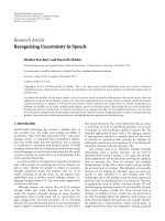
Fig. 5. An analog implementation using the proposed fast recursive drive-response mecha-
nism of the Lorenz system for the special case when using k
21
= 1 and k
31
= 0.

The experimental results for the synchronization process are illustrated in Fig. (6), where it
evident that the response system is capable of generating faithful estimates of the states of
the transmitter with the help of one driving signal.

quently adding more nonlinearities into the system. To investigate the practicality of the
design, a simple version of the design is now implemented in analog hardware using k
21
= 1
and k
31
= 0. The resulting system is governed by Eq. (14) and is illustrated by the Simulink
block diagram, shown in Fig. (4).

33
122
2
13213
13122
2133
31212
211
ˆ
ˆ
ˆ
ˆ
ˆˆˆ
)1(
ˆˆ
)1(
ˆ
fx
xfx
xffxf

xfxff
xxxx
xxxxx
xxx





















(14)

Fig. 4. A Simulink model for the simulation and implementation of Eq. (14) for the special

case when k
21
= 1 and k
31
= 0.

3.2 Practical considerations in the implementation phase
To meet practical considerations when implementing the drive-response system using ana-
log hardware, it will be required to adjust the peak values of the signals to fall within the
saturation levels imposed by the power supply and, in addition, to change the frequency
Robust Designs of Chaos-Based Secure Communication Systems 423

band of the system to conform to that of the signals involved, e.g. the transmitted secret
message in the case of secure communication systems. This can be achieved by using the
linear transformation in Eq. (15) that results in the modified system depicted by Eq. (16) for
which saturation nonlinearity is avoided.

3322
321
ˆ
1.0
ˆ
and ,
ˆ
2.0
ˆ
,1.0 ,2.0 ,2.0
/
fgfg
xwxvxu

t
t





(15)

3
2
2
233
322
ˆˆ
ˆˆ
5.2
ˆ
5.2
ˆˆ
)1(
ˆ
10
ˆ
)1(
ˆ
5.2
10
gw
ugv

ugugg
ugugg
uvww
uwvuv
vuu






















(16)

R1

100 kΩ
R2
100 kΩ
R3
100 kΩ
R4
100 kΩ
R5
100 kΩ
C1
1nF
IC= 5V
R6
100 kΩ
R7
280 kΩ
R8
100 kΩ
C2
1nF
Y
X
Y
X
R9
1MΩ
R10
100 kΩ
R11
100 kΩ

R12
25k Ω
R13
100 kΩ
C3
1nF
R14
375 kΩ
U1A
LF3 53H
3
2
4
8
1
U1B
LF3 53H
5
6
4
8
7
U2A
LF3 53H
3
2
4
8
1
U2B

LF3 53H
5
6
4
8
7
U3A
LF3 53H
3
2
4
8
1
U3B
LF3 53H
5
6
4
8
7
U7A
LF3 53H
3
2
4
8
1
R29
100 kΩ
R30

100 kΩ
R31
100 kΩ
R27
100 kΩ
R28
200 kΩ
U4A
LF3 53H
3
2
4
8
1
U4B
LF3 53H
5
6
4
8
7
R17
100 kΩ
C4
1nF
R19
90. 909 1kΩ
R18
100 kΩ
U5A

LF3 53H
3
2
4
8
1
R15
100 kΩ
R16
270 kΩ
Y
X
U5B
LF3 53H
5
6
4
8
7
R22
100 kΩ
C5
1nF
R26
375 kΩ
R25
100 kΩ
U6A
LF3 53H
3

2
4
8
1
R20
100 kΩ
R21
25k Ω
Y
X
R23
100 kΩ
R24
25k Ω
Y
X
U6B
LF3 53H
5
6
4
8
7
XSC 1
A B
G
T
XSC 2
A B
G

T
XSC 3
A B
G
T
XSC 4
A B
G
T
u - v
v - v
^
u - w
u
v
w
^
w - w
^
v
^
w
^

Fig. 5. An analog implementation using the proposed fast recursive drive-response mecha-
nism of the Lorenz system for the special case when using k
21
= 1 and k
31

= 0.

The experimental results for the synchronization process are illustrated in Fig. (6), where it
evident that the response system is capable of generating faithful estimates of the states of
the transmitter with the help of one driving signal.

quently adding more nonlinearities into the system. To investigate the practicality of the
design, a simple version of the design is now implemented in analog hardware using k
21
= 1
and k
31
= 0. The resulting system is governed by Eq. (14) and is illustrated by the Simulink
block diagram, shown in Fig. (4).

33
122
2
13213
13122
2133
31212
211
ˆ
ˆ
ˆ
ˆ
ˆˆˆ
)1(
ˆˆ

)1(
ˆ
fx
xfx
xffxf
xfxff
xxxx
xxxxx
xxx





















(14)

Fig. 4. A Simulink model for the simulation and implementation of Eq. (14) for the special
case when k
21
= 1 and k
31
= 0.

3.2 Practical considerations in the implementation phase
To meet practical considerations when implementing the drive-response system using ana-
log hardware, it will be required to adjust the peak values of the signals to fall within the
saturation levels imposed by the power supply and, in addition, to change the frequency
Recent Advances in Signal Processing424

50 60 70 80 90 100
-4
-2
0
2
4
Time
(
ms
)
u

0 500 1000 1500 2000 2500 3000

f
d
= 537 Hz
Frequency (Hz)
P
w

(a) (b)
50 60 70 80 90 100
-0.1
0
0.1
Time (ms)
s(t)

0 50 100 150 200 250 300
f
s
= 50 Hz
Frequency (Hz)
P
w

(c) (d)
Fig. 8. The driving signal, u = 0.2x
1
and its power spectrum for the case when

= 1 ms are
shown in (a) and (b) respectively. The sample transmitted secret message and its power

spectrum are illustrated in (c) and (d) respectively.

Both the encryption and decryption functions are given in Eq. (17), where only x
2
was used
to construct the nonlinear scrambling. The decryption function should settle very fast to the
inverse of the encryption function, once synchronization is achieved.

)()1(),,(
2
2
2
2
tsxxtsXE 

)
ˆ
1/()
ˆ
),,((),,
ˆ
()(
ˆ
2
2
2
2
xxtsXEtsXDts 

(17)

For improved security, the amplitude of the secret message should be much smaller than
that of x
2
. For simplicity and without loss of generality, a sinusoidal signal is chosen for
illustration purposes with the form s(t) = A
s
sin (2

f
s
t), f
s
<< f
d
, for which the frequency, f
s
, is
chosen to be much less than the dominant frequency of the chaotic attractor of the transmit-
ter, f
d
, to ensure minimum effects of transients. Figure (9) illustrate the improvements in the
decryption error, e(t) = D(t) – s(t), when using the conventional and the fast recursive meth-
ods for synchronization, where the absolute value of e(t) over five periods of the transmitted
signal was found to reduce from 4.2% to 1.7% respectively.

0 1 2 3 4 5 6 7 8 9 10
-1
-0.5
0

0.5
1
Time (ms)
e(t)

k
21
= k
31
= 0
k
21
= k
31
= 1

Fig. 9. A comparative study of the transient effects on the decryption error.

Figure (10) illustrate the complete response of the communication system, demonstrating
the satisfactory performance of the proposed technique.

(a) (b)
Fig. 6. The steady state results of the synchronization, illustrating perfect matching between
the states of both the drive and response systems for x
2
and x

3
in (a) and (b) respectively.

3.3 Case study I
Constructing a secure communication system is now investigated where the fast recursive
synchronization mechanism is now combined with a nonlinear encryption function, E, at the
transmitter in order to hide the secret message s(t). At The receiver side, a decryption func-
tion, D, reverses the scrambling process to reconstruct the original message. Figure (7) illus-
trates this idea where the frequency band of both the transmitter and the receiver are ad-
justed using the time scaling factor,

, and the public channel is used to transmit both x
1
(the
driving signal necessary for synchronization), and E , the encrypted secret message, which is
similar to the work done in (Jiang, 2002; Solak, 2004; Zaher, 2009). Figure (8) illustrate the
power spectrum analysis for both the secret message and the chaotic transmitter.

Fig. 7. A block diagram representation of the chaos-based secure communication system.
Robust Designs of Chaos-Based Secure Communication Systems 425

50 60 70 80 90 100
-4
-2
0
2
4
Time
(

ms
)
u

0 500 1000 1500 2000 2500 3000
f
d
= 537 Hz
Frequency (Hz)
P
w

(a) (b)
50 60 70 80 90 100
-0.1
0
0.1
Time (ms)
s(t)

0 50 100 150 200 250 300
f
s
= 50 Hz
Frequency (Hz)
P
w

(c) (d)
Fig. 8. The driving signal, u = 0.2x

1
and its power spectrum for the case when

= 1 ms are
shown in (a) and (b) respectively. The sample transmitted secret message and its power
spectrum are illustrated in (c) and (d) respectively.

Both the encryption and decryption functions are given in Eq. (17), where only x
2
was used
to construct the nonlinear scrambling. The decryption function should settle very fast to the
inverse of the encryption function, once synchronization is achieved.

)()1(),,(
2
2
2
2
tsxxtsXE 

)
ˆ
1/()
ˆ
),,((),,
ˆ
()(
ˆ
2
2

2
2
xxtsXEtsXDts 

(17)

For improved security, the amplitude of the secret message should be much smaller than
that of x
2
. For simplicity and without loss of generality, a sinusoidal signal is chosen for
illustration purposes with the form s(t) = A
s
sin (2

f
s
t), f
s
<< f
d
, for which the frequency, f
s
, is
chosen to be much less than the dominant frequency of the chaotic attractor of the transmit-
ter, f
d
, to ensure minimum effects of transients. Figure (9) illustrate the improvements in the
decryption error, e(t) = D(t) – s(t), when using the conventional and the fast recursive meth-
ods for synchronization, where the absolute value of e(t) over five periods of the transmitted
signal was found to reduce from 4.2% to 1.7% respectively.

0 1 2 3 4 5 6 7 8 9 10
-1
-0.5
0
0.5
1
Time (ms)
e(t)

k
21
= k
31
= 0
k
21
= k
31
= 1

Fig. 9. A comparative study of the transient effects on the decryption error.

Figure (10) illustrate the complete response of the communication system, demonstrating
the satisfactory performance of the proposed technique.

(a) (b)
Fig. 6. The steady state results of the synchronization, illustrating perfect matching between
the states of both the drive and response systems for x
2
and x
3
in (a) and (b) respectively.

3.3 Case study I
Constructing a secure communication system is now investigated where the fast recursive
synchronization mechanism is now combined with a nonlinear encryption function, E, at the
transmitter in order to hide the secret message s(t). At The receiver side, a decryption func-
tion, D, reverses the scrambling process to reconstruct the original message. Figure (7) illus-
trates this idea where the frequency band of both the transmitter and the receiver are ad-
justed using the time scaling factor,

, and the public channel is used to transmit both x
1
(the
driving signal necessary for synchronization), and E , the encrypted secret message, which is
similar to the work done in (Jiang, 2002; Solak, 2004; Zaher, 2009). Figure (8) illustrate the
power spectrum analysis for both the secret message and the chaotic transmitter.

Fig. 7. A block diagram representation of the chaos-based secure communication system.
Recent Advances in Signal Processing426

(a)
0 10 20 30 40 50 60 70 80 90 100
-0.2

-0.1
0
0.1
0.2
Time
(
ms
)
s , D

s(t)
D(t)

(b)
0 10 20 30 40 50 60 70 80 90 100
-0.2
-0.1
0
0.1
0.2
Time
(
ms
)
s , D

s(t)
D(t)

(c)
0 10 20 30 40 50 60 70 80 90 100
-0.2
-0.1
0
0.1
0.2
Time (ms)
s , D

s(t)
D(t)

(d)
0 10 20 30 40 50 60 70 80 90 100
-0.2
-0.1
0
0.1
0.2
Time
(
ms
)
s , D

s(t)

D(t)

Fig. 11. The sensitivity to synchronization multiplicative errors is exemplified in (a) and (b),
corresponding to  = 0.01 and 0.05 respectively and to synchronization additive errors in (c)
and (d), corresponding to  = 0.02 and 0.1 respectively (f
s
= 50 Hz).

(a)
0 10 20 30 40 50 60 70 80 90 100
-0.2
-0.1
0
0.1
0.2
Time
(
ms
)
s , D

s(t)
D(t)

(b)
0 10 20 30 40 50 60 70 80 90 100
-0.2
-0.1
0

0.1
0.2
Time
(
ms
)
s , D

s(t)
D(t)

(c)
0 10 20 30 40 50 60 70 80 90 100
-0.2
-0.1
0
0.1
0.2
Time (ms)
s , D

s(t)
D(t)

(d)
0 10 20 30 40 50 60 70 80 90 100
-0.2
-0.1

0
0.1
0.2
Time
(
ms
)
s , D

s(t)
D(t)

Fig. 12. The sensitivity to synchronization errors, when f
s
= 500 Hz.

(a)
0 10 20 30 40 50 60 70 80 90 100
-20
0
20
Time
(
ms
)
x
1

(b)

0 10 20 30 40 50 60 70 80 90 100
-0.2
-0.1
0
0.1
0.2
Time
(
ms
)
S(t)

(c)
0 10 20 30 40 50 60 70 80 90 100
0
200
400
600
Time
(
ms
)
E(t)

(d)
0 10 20 30 40 50 60 70 80 90 100
-0.2
-0.1
0
0.1

0.2
Time
(
ms
)
D(t)

(e)
0 10 20 30 40 50 60 70 80 90 100
-0.2
-0.1
0
0.1
0.2
Time
(
ms
)
e(t)

Fig. 10. Signals profile of the secure communication system. The synchronization signal, x
1
,
is shown in (a), the secret message, s(t), in (b), the encrypted signal, E(t), in (c), the decrypted
signal, D(t), in (d), and finally the decryption error, e(t), in (e).

3.4 Sensitivity and security analysis for case study I
The encryption function considered in the previous section depends only on x
2
and conse-

quently the decryption error is sensitive to synchronization errors. To investigate this prob-
lem, two cases will be considered that include both multiplicative and additive errors. These
errors can result from channel noise, modelling errors, or both. The mathematical represen-
tation of this problem is described in Eq. (18).

δ
ˆ
:error Additive
)1(
ˆ
:error tiveMultiplica
22
22


xx
xx

(18)

Figure (11) shows the synchronization error problem for the case when the transmitted
message is an analog sinusoidal signal for different values of  and , illustrating the strong
dependence of the decryption error on the synchronization errors. Figures (12) and (13)
confirm the same result when the frequency of the transmitted message is comparable to
and much greater than the dominant frequency of the chaotic attractor of the transmitter,
corresponding to 500 Hz and 5 kHz respectively.
Robust Designs of Chaos-Based Secure Communication Systems 427

(a)
0 10 20 30 40 50 60 70 80 90 100

-0.2
-0.1
0
0.1
0.2
Time
(
ms
)
s , D

s(t)
D(t)

(b)
0 10 20 30 40 50 60 70 80 90 100
-0.2
-0.1
0
0.1
0.2
Time
(
ms
)
s , D

s(t)

D(t)

(c)
0 10 20 30 40 50 60 70 80 90 100
-0.2
-0.1
0
0.1
0.2
Time (ms)
s , D

s(t)
D(t)

(d)
0 10 20 30 40 50 60 70 80 90 100
-0.2
-0.1
0
0.1
0.2
Time
(
ms
)
s , D

s(t)
D(t)

Fig. 11. The sensitivity to synchronization multiplicative errors is exemplified in (a) and (b),
corresponding to  = 0.01 and 0.05 respectively and to synchronization additive errors in (c)
and (d), corresponding to  = 0.02 and 0.1 respectively (f
s
= 50 Hz).

(a)
0 10 20 30 40 50 60 70 80 90 100
-0.2
-0.1
0
0.1
0.2
Time
(
ms
)
s , D

s(t)
D(t)

(b)
0 10 20 30 40 50 60 70 80 90 100
-0.2
-0.1

0
0.1
0.2
Time
(
ms
)
s , D

s(t)
D(t)

(c)
0 10 20 30 40 50 60 70 80 90 100
-0.2
-0.1
0
0.1
0.2
Time (ms)
s , D

s(t)
D(t)

(d)
0 10 20 30 40 50 60 70 80 90 100
-0.2

-0.1
0
0.1
0.2
Time
(
ms
)
s , D

s(t)
D(t)

Fig. 12. The sensitivity to synchronization errors, when f
s
= 500 Hz.

(a)
0 10 20 30 40 50 60 70 80 90 100
-20
0
20
Time
(
ms
)
x
1

(b)
0 10 20 30 40 50 60 70 80 90 100
-0.2
-0.1
0
0.1
0.2
Time
(
ms
)
S(t)

(c)
0 10 20 30 40 50 60 70 80 90 100
0
200
400
600
Time
(
ms
)
E(t)

(d)
0 10 20 30 40 50 60 70 80 90 100
-0.2
-0.1
0

0.1
0.2
Time
(
ms
)
D(t)

(e)
0 10 20 30 40 50 60 70 80 90 100
-0.2
-0.1
0
0.1
0.2
Time
(
ms
)
e(t)

Fig. 10. Signals profile of the secure communication system. The synchronization signal, x
1
,
is shown in (a), the secret message, s(t), in (b), the encrypted signal, E(t), in (c), the decrypted
signal, D(t), in (d), and finally the decryption error, e(t), in (e).

3.4 Sensitivity and security analysis for case study I
The encryption function considered in the previous section depends only on x
2

and conse-
quently the decryption error is sensitive to synchronization errors. To investigate this prob-
lem, two cases will be considered that include both multiplicative and additive errors. These
errors can result from channel noise, modelling errors, or both. The mathematical represen-
tation of this problem is described in Eq. (18).

δ
ˆ
:error Additive
)1(
ˆ
:error tiveMultiplica
22
22




xx
xx

(18)

Figure (11) shows the synchronization error problem for the case when the transmitted
message is an analog sinusoidal signal for different values of  and , illustrating the strong
dependence of the decryption error on the synchronization errors. Figures (12) and (13)
confirm the same result when the frequency of the transmitted message is comparable to
and much greater than the dominant frequency of the chaotic attractor of the transmitter,
corresponding to 500 Hz and 5 kHz respectively.
Recent Advances in Signal Processing428

(a)
0 20 40 60 80 100 120 140 160 180 200
-0.1
0
0.1
0.2
Time
(
ms
)
S(t)

(b)
0 20 40 60 80 100 120 140 160 180 200
0
200
400
600
Time (ms)
E(t)

(c)
0 20 40 60 80 100 120 140 160 180 200
-0.1
0
0.1
0.2
Time (ms)
S(t)

^

(d)
0 20 40 60 80 100 120 140 160 180 200
-0.2
-0.1
0
0.1
0.2
Time (ms)
e(t)

Fig. 15. The response of the intruder system showing the original secret message; s(t), its
encryption using only x
2
; E(t), the decrypted signal; D(t) superimposed on s(t), and the de-
cryption error; e(t), in (a), (b), (c), and (d) respectively.

Figure (15) shows a successful attack of an intruder for the case when the frequency of the
digital secret message, f
s
, was much less than that of the chaotic transmitter, f
d
. The same
argument applies when f
s
is much higher than f
d
as using a high-pass filter can isolate the
digital message; however, the effect of time delays and channel noise will be more obvious.

When f
s
and f
d
occupy the same frequency interval, it will not be possible to use filtering
techniques to separate them from each other. This fact will be used later in this chapter to
robustify the design of the secure communication system. It can be also demonstrated that it
is easier to break into the system and recover digital message rather than analog messages
because of the sensitivity of the later to noise.

3.5 Case study II
The aforementioned discussion requires modifying the encryption function at the transmit-
ter, depicted by Fig. (7) and Eq. (17), to make it more difficult for the intruder to break the
security of the communication system. This will be the topic of the next section; but first the
parameter modulation technique is now investigated as a possible replacement to encryp-
tion. Figure (16) shows a Simulink model for such purpose, where the secret message is used
directly to modulate the value of

. The analysis carried out in (Álvarez, 2004; Zaher, 2009)
is now used to prove that it is easy to recover the original digital signal using low-pass filter-
ing followed by thresholding, without having to know the structure of the transmitter or to
synchronizer a receiver model with that of the transmitter. Figure (17) illustrate the results
of such system.

(a)
90 91 92 93 94 95 96 97 98 99 100
-0.2
-0.1
0
0.1

0.2
Time
(
ms
)
s, D

s(t)
D(t)

(b)
90 91 92 93 94 95 96 97 98 99 100
-0.2
-0.1
0
0.1
0.2
Time
(
ms
)
s, D

s(t)
D(t)

(c)
90 91 92 93 94 95 96 97 98 99 100

-0.2
-0.1
0
0.1
0.2
Time
(
ms
)
s, D

s(t)
D(t)

(d)
90 91 92 93 94 95 96 97 98 99 100
-0.2
-0.1
0
0.1
0.2
Time
(
ms
)
s, D

s(t)

D(t)

Fig. 13. The sensitivity to synchronization errors, when f
s
= 5 kHz.

Figures (11-13) show that the effect of additive error is more critical than multiplicative
error. In addition, as the frequency of the transmitted signal increases the decrypted signal
deteriorates, as transient effects will persist. Although the envelope of the transmitted signal
can be clearly seen from the distorted decrypted signal, for the transmission of digital sig-
nals this is not the case. To complete the analysis of the communication system, its security
is investigated by assuming that an intruder picks up the encrypted message from the com-
munication channel and then tries to isolate the digital secret message by employing a two-
stage process consisting of low-pass filtering and thresholding. This is illustrated in Fig. (14).

Fig. 14. A Simulink model illustrating the possibility of breaking the security of the commu-
nication system via utilizing simple filtering techniques.
Robust Designs of Chaos-Based Secure Communication Systems 429

(a)
0 20 40 60 80 100 120 140 160 180 200
-0.1
0
0.1
0.2
Time
(
ms
)
S(t)

(b)
0 20 40 60 80 100 120 140 160 180 200
0
200
400
600
Time (ms)
E(t)

(c)
0 20 40 60 80 100 120 140 160 180 200
-0.1
0
0.1
0.2
Time (ms)
S(t)
^

(d)
0 20 40 60 80 100 120 140 160 180 200
-0.2
-0.1
0
0.1
0.2
Time (ms)
e(t)

Fig. 15. The response of the intruder system showing the original secret message; s(t), its
encryption using only x
2
; E(t), the decrypted signal; D(t) superimposed on s(t), and the de-
cryption error; e(t), in (a), (b), (c), and (d) respectively.

Figure (15) shows a successful attack of an intruder for the case when the frequency of the
digital secret message, f
s
, was much less than that of the chaotic transmitter, f
d
. The same
argument applies when f
s
is much higher than f
d
as using a high-pass filter can isolate the
digital message; however, the effect of time delays and channel noise will be more obvious.
When f
s
and f
d
occupy the same frequency interval, it will not be possible to use filtering
techniques to separate them from each other. This fact will be used later in this chapter to
robustify the design of the secure communication system. It can be also demonstrated that it
is easier to break into the system and recover digital message rather than analog messages
because of the sensitivity of the later to noise.

3.5 Case study II
The aforementioned discussion requires modifying the encryption function at the transmit-

ter, depicted by Fig. (7) and Eq. (17), to make it more difficult for the intruder to break the
security of the communication system. This will be the topic of the next section; but first the
parameter modulation technique is now investigated as a possible replacement to encryp-
tion. Figure (16) shows a Simulink model for such purpose, where the secret message is used
directly to modulate the value of

. The analysis carried out in (Álvarez, 2004; Zaher, 2009)
is now used to prove that it is easy to recover the original digital signal using low-pass filter-
ing followed by thresholding, without having to know the structure of the transmitter or to
synchronizer a receiver model with that of the transmitter. Figure (17) illustrate the results
of such system.

(a)
90 91 92 93 94 95 96 97 98 99 100
-0.2
-0.1
0
0.1
0.2
Time
(
ms
)
s, D

s(t)
D(t)

(b)

90 91 92 93 94 95 96 97 98 99 100
-0.2
-0.1
0
0.1
0.2
Time
(
ms
)
s, D

s(t)
D(t)

(c)
90 91 92 93 94 95 96 97 98 99 100
-0.2
-0.1
0
0.1
0.2
Time
(
ms
)
s, D

s(t)
D(t)

(d)
90 91 92 93 94 95 96 97 98 99 100
-0.2
-0.1
0
0.1
0.2
Time
(
ms
)
s, D

s(t)
D(t)

Fig. 13. The sensitivity to synchronization errors, when f
s
= 5 kHz.

Figures (11-13) show that the effect of additive error is more critical than multiplicative
error. In addition, as the frequency of the transmitted signal increases the decrypted signal
deteriorates, as transient effects will persist. Although the envelope of the transmitted signal
can be clearly seen from the distorted decrypted signal, for the transmission of digital sig-
nals this is not the case. To complete the analysis of the communication system, its security
is investigated by assuming that an intruder picks up the encrypted message from the com-

munication channel and then tries to isolate the digital secret message by employing a two-
stage process consisting of low-pass filtering and thresholding. This is illustrated in Fig. (14).

Fig. 14. A Simulink model illustrating the possibility of breaking the security of the commu-
nication system via utilizing simple filtering techniques.
Recent Advances in Signal Processing430

4. Identifying the Parameters of Chaotic Systems
A feasible improvement to chaos-based cryptosystems can be made via making the encryp-
tion process a function of one or more of the parameters of the chaotic transmitter and not
only the states. A possible candidate is given in Eq. (19) and is illustrated in Fig. (18).

)()(),,,(
2
2
22
2
tsxxtsXE 


)
ˆ
/()
ˆ
),,,((),,,
ˆ
()(
ˆ
2
2

22
2
xxtsXEtsXDts 


(19)

Fig. 18. A block diagram representation of the modified chaos-based secure communication
system for which the encryption function depends on

.

Although the scrambling of the message is improved, this has the effect of increasing the
message strength; thus making it more vulnerable to be digged out of the encrypted signal
using simple filtering techniques. This is illustrated in Fig. (19) using the same filtering tech-
nique discussed in Sec. (3.5). Figure (20) shows a Simulink model for implementing Eq. (19),
while Figs. (21) and (22) show the effect of guessing

by the intruder, assuming that only
the model of the transmitter and the structure of the encryption function are known.

(a)
0 20 40 60 80 100 120 140 160 180 200
0
200
400
600
Time

(
ms
)
E(t)

(b)
0 20 40 60 80 100 120 140 160 180 200
-0.1
0
0.1
0
.
2
Time
(
ms
)
S(t)
^

Fig. 19. The response of the modified intruder system showing E(t) that depends on both x
2

and

; and the decrypted signal, D(t), superimposed on s(t), in (a), (b) respectively.

Fig. 16. A Simulink block diagram illustration of using simple filtering techniques to break
into a chaos-based communication system that relies on parameter modulation.

(a)
0 20 40 60 80 100 120
5
7.5
10
12.5
15
Time
(
s
)
S(t)

(b)
0 20 40 60 80 100 120
-20
0
20
Time (s)
x
1

(c)
0 20 40 60 80 100 120
0
20
40
60
80

100
Time
(
s
)
x
1
2
LPF

(d)
0 20 40 60 80 100 120
5
7.5
10
12.5
15
Time (s)
S(t)
^

Fig. 17. The response of the intruder system showing the original secret message; s(t), its
encryption; E(t), the output of the low-pass filter, and the reconstructed message, superim-
posed on s(t), in (a), (b), (c), and (d) respectively.

Robust Designs of Chaos-Based Secure Communication Systems 431

4. Identifying the Parameters of Chaotic Systems
A feasible improvement to chaos-based cryptosystems can be made via making the encryp-
tion process a function of one or more of the parameters of the chaotic transmitter and not

only the states. A possible candidate is given in Eq. (19) and is illustrated in Fig. (18).

)()(),,,(
2
2
22
2
tsxxtsXE 


)
ˆ
/()
ˆ
),,,((),,,
ˆ
()(
ˆ
2
2
22
2
xxtsXEtsXDts 


(19)

Fig. 18. A block diagram representation of the modified chaos-based secure communication

system for which the encryption function depends on

.

Although the scrambling of the message is improved, this has the effect of increasing the
message strength; thus making it more vulnerable to be digged out of the encrypted signal
using simple filtering techniques. This is illustrated in Fig. (19) using the same filtering tech-
nique discussed in Sec. (3.5). Figure (20) shows a Simulink model for implementing Eq. (19),
while Figs. (21) and (22) show the effect of guessing

by the intruder, assuming that only
the model of the transmitter and the structure of the encryption function are known.

(a)
0 20 40 60 80 100 120 140 160 180 200
0
200
400
600
Time
(
ms
)
E(t)

(b)
0 20 40 60 80 100 120 140 160 180 200
-0.1
0
0.1

0
.
2
Time
(
ms
)
S(t)
^

Fig. 19. The response of the modified intruder system showing E(t) that depends on both x
2

and

; and the decrypted signal, D(t), superimposed on s(t), in (a), (b) respectively.

Fig. 16. A Simulink block diagram illustration of using simple filtering techniques to break
into a chaos-based communication system that relies on parameter modulation.

(a)
0 20 40 60 80 100 120
5
7.5
10
12.5
15
Time
(

s
)
S(t)

(b)
0 20 40 60 80 100 120
-20
0
20
Time (s)
x
1

(c)
0 20 40 60 80 100 120
0
20
40
60
80
100
Time
(
s
)
x
1
2
LPF

(d)
0 20 40 60 80 100 120
5
7.5
10
12.5
15
Time (s)
S(t)
^

Fig. 17. The response of the intruder system showing the original secret message; s(t), its
encryption; E(t), the output of the low-pass filter, and the reconstructed message, superim-
posed on s(t), in (a), (b), (c), and (d) respectively.

Recent Advances in Signal Processing 2011 Part 13 pot

Tài liệu liên quan

Tài liệu bạn tìm kiếm đã sẵn sàng tải về