Báo cáo hóa học: " Research Article Detection and Localization of Transient Sources: Comparative Study of Complex-Lag Distribution Concept Versus Wavelets and Spectrogram-Based Methods" pot

Hindawi Publishing Corporation
EURASIP Journal on Advances in Signal Processing
Volume 2009, Article ID 864185, 12 pages
doi:10.1155/2009/864185
Research Article
Detection and Localization of Transient Sources:
Comparative Study of Complex-Lag Distribution Concept Versus
Wavelets and Spectrogram-Based Methods
Bertrand Gottin,
1
Cornel Ioana,
1
Jocelyn Chanussot,
1
Guy D’Urso,
2
and Thierry Espilit
3
1
GIPSA-Lab, Grenoble INP, Domaine Universitaire Saint-Martin d’Heres, 38402 Saint-Martin d’Heres, France
2
Research and Development of EDF, 78401 Chatou, France
3
Research and Development of EDF, 77250 Moret sur Loing, France
Correspondence should be addressed to Bertrand Gottin,
Received 11 June 2009; Accepted 25 September 2009
Recommended by A. Enis Cetin
The detection and localization of transient signals is nowadays a typical point of interest when we consider the multitude of
existing transient sources, such as electrical and mechanical systems, underwater environments, audio domain, seismic data, and
so forth. In such fields, transients carry out a lot of information. They can correspond to a large amount of phenomena issued
from the studied problem and important to analyze (anomalies and perturbations, natural sources, environmental singularities,

). They usually occur randomly as brief and sudden signals, such as partial discharges in electrical cables and transformers tanks.
Therefore, motivated by advanced and accurate analysis, efficient tools of transients detection and localization are of great utility.
Higher order statistics, wavelets and spectrogram distributions are well known methods which proved their efficiency to detect and
localize transients independently to one another. However, in the case of a signal composed by several transients physically related
and with important energy gap between them, the tools previously mentioned could not detect efficiently all the transients of the
whole signal. Recently, the generalized complex time distribution concept has been introduced. This distribution offers access to
highly concentrated representation of any phase derivative order of a signal. In this paper, we use this improved phase analysis
tool to define a new concept to detect and localize dependant transients taking regard to the phase break they cause and not their
amplitude. ROC curves are calculated to analyze and compare the performances of the proposed methods.
Copyright © 2009 Bertrand Gottin et al. This is an open access article distributed under the Creative Commons Attribution
License, which permits unrestricted use, distribution, and reproduction in any medium, provided the original work is properly
cited.
1. Introduction
Transient signals can be globally defined as impulsive or
very short duration signals often with oscillations. These
signals exist in many different applications and systems from
underwater acoustic [1] with opportunity sources to audio
signals with sound attacks [2] or electrical systems with
partial discharges and faults in cables [3]. The main pro-
cessing done on this type of signal aims to detect them and
localize their source in multisensor configuration. One issue
point concerning transient signals is that they are typically
defined on very few samples and are difficult to modelize by
asymptotic approach. Consequently, their characterization
remains a very challenging goal of increasing interest. Until
now, several signal processing tools such as Higher-Order
Statistics (HOS), Wavelets (WVT) coefficients, and well-
known Time-Frequency analysis by Spectrogram are widely
used to perform the goals of detection and localization.
The HOS are very suitable to detect transients drowned

in additive white Gaussian noise. The HOS give high
value statistics for non-Gaussian components as transients,
whereas all Gaussian parts of the signal have higher-order
statistics very closed to zero [4, 5]. Wavelet coefficients and
spectrogram are based on energy criteria and give high
energetical value signatures where transient components
occur [6, 7]. One of the common points of these approaches
is the use of energy coefficients to prove the transients
detection. Alternatively, the transients could be detected
via the changes of signal instantaneous phase. Hence, one
promising approach consists of analyzing the instantaneous
2 EURASIP Journal on Advances in Signal Processing
phase derivatives of the studied signal and to detect the
transitions as the signal parts which provide significant
values of phase derivatives at several orders. Recently, for
phase derivatives analysis, the time-frequency distribution
based on complex lag arguments has been introduced [8, 9].
This distribution is able to reduce inner interferences terms
which appear when studying nonlinear TF components. It
also offers access to an instantaneous law representation of
any phase derivative order.
Unlikely to HOS, WVT, and Spectrogram, this concept of
complex-lag distribution focuses directly on the phase law of
the signal with no regard to its amplitude. Therefore, in a task
of transients detection, when the amplitude of the transient
is too low, the statistics obtained by HOS (Skewness, Kurtosis
or fourth-order cumulant) as well as WVT coefficients could
be too weak and not enough significant for detection. In
the same way, the spectrogram distribution could miss
low amplitude transients masked by other transients or

components of strong amplitude. Using the complex-lag
distribution, despite low amplitude signal, the phase break
due to the transient remains significant and visible for
detection in the “Time-Phase Derivatives” representation
plane.
In this paper, we consider transient signals from a
multipath configuration. This configuration is encountered
in many application areas such as electrocardiograms (EKG),
underwater acoustic, seismic, and so forth. A good illus-
trative case of such configuration signals is the one of
signals from reflectometry studies using Gaussian pulse
transmission in electric power cables. This reflectometry
signal is composed by the emitted pulse and several other
pulses due to some reflections on particular cable spots (end
of cable, junction points, faults points) [10]. These reflection
pulses come back to the cable reflectometry transmission
point with some delay, amplitude attenuation, and phase
shift.
The paper is organized as follows. In Section 2 apresen-
tation of the complex time distribution concept is done. The
capability of each method to deal with full detection and
localization of transients contained in typical reflectometry
signalsispresentedinSection 3.WeconcludeinSection 4.
2. Time-Frequency Distribution Based on
Complex Lag Arguments
The concept of complex lag distributions has been intro-
duced in [8] as a way for inner interferences reduction with
respect to Wigner distribution. Recently, this concept has
been generalized in order to focus on arbitrary instantaneous
phase derivative of a signal [9]. Let us consider the signal

defined as
s
(
t
)
= A ·e
jφ
(
t
)
. (1)
The case of A depending of t can also be addressed since
the effect of slowly varying amplitude is “visible” on the
instantaneous phase. Otherwise, after a signal normalization,
we can consider A
= 1.
−1+1
Re
Im
Figure 1: Lag coefficients taken on the real axis.
In order to better understand the concept of complex lag
distribution and its generalization, applied on such a signal,
let us introduce the very well-known Wigner distribution
with appropriate analysis of its moment and lags definition.
2.1. The Wigner Ville Distribution. The Wigner Ville distri-
bution of a signal s(t) is by definition [11]:
WVD
(
t, ω
)

= F
τ
⎡
⎢
⎢
⎢
⎣
M
wv
(
t,τ
)
  
s

t +
τ
2

s
∗

t −
τ
2

⎤
⎥
⎥
⎥

⎦
. (2)
This corresponds to the Fourier transform, with respect
to the lag variable τ, of a higher-order moment denoted
M
wv
(t, τ). As illustrated in Figure 1,thismomentiscalcu-
lated using two lag coefficients taken on the real axis.
For a signal defined in (1), the expression of the moment
becomes
M
wv
(
t, τ
)
= e
j
[
φ
(
t+τ/2
)
−φ
(
t−τ/2
)
]
. (3)
Let us express the signal phase law in terms of Taylor
series expansion:

φ

t +
τ
2

=
+φ

(
t
)
τ
2
1
1!
+ φ
(
2
)
(
t
)
τ
2
2
2
2!
+ φ
(

3
)
(
t
)
τ
3
2
3
3!
+
···,
φ

t −
τ
2

=−
φ

(
t
)
τ
2
1
1!
+ φ
(

2
)
(
t
)
τ
2
2
2
2!
−φ
(
3
)
(
t
)
τ
3
2
3
3!
+
···.
(4)
Using the derivation results above, the expression (3)
becomes
M
wv
(

t, τ
)
= e
jφ

(
t
)
τ
×e
j
[
φ
(
3
)
(
t
)
(
τ
3
/2
2
3!
)
+···
]
. (5)
By substituting (5)in(2), we obtain a new analytical expres-

sion (6) of the WVD defining it as an ideally concentrated
representation of the Instantaneous Frequency Law (IFL),
but degraded because of the convolution with a spreading
factor.
WVD
(
t, ω
)
= δ

ω −φ

(
t
)

∗
ω
F
τ

e
jQ
wv
(
t,τ
)

,(6)
where Q

wv
is the spread function defined as
Q
wv
(
t, τ
)
= φ
(
3
)
(
t
)
τ
3
2
2
3!
+ φ
(
5
)
(
t
)
τ
5
2
4

5!
+ φ
(
7
)
(
t
)
τ
7
2
6
7!
···.
(7)
EURASIP Journal on Advances in Signal Processing 3
−1+1
Re
Im
−j
+j
Figure 2: Lag coefficients taken on the real and imaginary axis.
From this spread function expression, it is easy to understand
that the concentration of the WV representation for a
chirp signal (polynomial phase law of second order) will be
optimal in so far as all φ’s derivates terms in Q
wv
will be equal
to zero.
2.2. The Complex-Time Distribution. The Complex-Time

distribution of a signal s(t) is by definition [8]:
CTD
(
t, ω
)
= F
τ
⎡
⎢
⎢
⎢
⎣
M
ct
(
t,τ
)
  
s

t +
τ
4

s
∗

t −
τ
4


s
−j

t + j
τ
4

s
j

t − j
τ
4

⎤
⎥
⎥
⎥
⎦
.
(8)
In the same way as WVD, this corresponds to the Fourier
transform, with respect of the lag variable τ,ofahigher
order moment denoted M
ct
(t, τ). As illustrated in Figure 2,
this moment is in this case of order four and calculated
using two lag coefficients taken on the real axis as well as
on the imaginary axis, hence the concept of “complex-time

arguments emerges”.
Following the same frame of analysis described in
Section 2.1 leads to a new expression of CTD defined with the
same form as (6). The spread function for this distribution is
[8]
Q
ct
(
t, τ
)
= φ
(
5
)
(
t
)
τ
5
4
4
5!
+ φ
(
9
)
(
t
)
τ

9
4
8
9!
+ φ
(
13
)
(
t
)
τ
13
4
12
13!
···.
(9)
Defining a distribution using well-chosen “complex-lag”
arguments (+ j and
−j on the imaginary axis) involves
a significant decreasing of the spread factor. The first
term of Q
ct
(t, τ) is of the fifth order. The terms of phase
derivatives of order 3, 7, 11, are completely eliminated
and all remaining terms are much more reduced with
respect to the ones in the Wigner distribution. The Complex
Time Distribution improves the concentration of the IFL
representation comparing to the one obtained by Wigner

Distribution (Figure 4). In the case of a nonlinear and rapidly
varying TF structure, the inner interferences are strongly
reduced.
2.3. The Generalized Complex-time Distribution. Recently,
a generalization of the concept of CTD has been defined
[9]. The starting point of this generalization procedure was
p =2
p
= 1
Re
Im
p
= 0
p
= N −1
θ
t
τ
Figure 3: The complex lag coordinates.
the Cauchy’s integral formula [12]. Using this theorem,
it is possible to compute the Kth order derivative of the
instantaneous phase as
φ
(
K
)
(
t
)
=

K!
2πj

γ
φ
(
z
)
(
z
−t
)
K+1
dz. (10)
This relation shows the interest of the complex time concept:
the Kth order derivate of function φ at instant t (which could
correspond to one signal singularity) can be computed as the
complex integral over the integration path γ defined, in the
complex plane, around this point. Applying the theory of
Cauchy’s integral theorem [12] and considering a circle as
integration path, the expression (10)becomes[9]
φ
(
K
)
(
t
)
=
K!

2πτ
K

2π
0
φ

t + τe
jθ

e
−jKθ
dθ. (11)
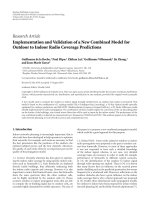
As illustrated in Figure 3, the discrete version of (11)is
defined for θ
= 2πp/N and p = 0, , N − 1, where N is the
number of discrete values of the angle θ (expression (12)).
φ
(
K
)
(
t
)
=
K!
Nτ
K
N
−1


p=0
φ

t + τe
j
(
2πp/N
)

e
−j
(
2πpK/N
)
+ ε, (12)
where ε is the discretization error.
Using the property of the unitary roots ω
N,p
= e
j2πp/N
and the variable change τ ←
K

τ(K!/N), the expression (12)
becomes (cf. Appendix A)
N−1

p=0
φ

⎛
⎝
t + ω
N,p
K

τ
K!
N
⎞
⎠
ω
N−K
N,p
= φ
(
K
)
(
t
)
τ + Q
(
t, τ
)
, (13)
where Q is the spread function defined as [9]:
Q
(
t, τ

)
= N
+∞

r=1
φ
(
Nr+K
)
(
t
)
τ
Nr/K+1
(
Nr + K
)
!

K!
N

Nr/K+1
. (14)
As indicated by (13)and(14), the sum of the phase
samples defined in the complex coordinates (left side of
(13)) is linear depending on τ if the φ’s derivates of orders
greater than N + K are0.Inordertoexploitthispropertywe
4 EURASIP Journal on Advances in Signal Processing
define the generalized complex-lag moment (GCM) of s as

the operation leading to (13):
GCM
K
N
[
s
]
(
t, τ
)
=
N−1

p=0
s
ω
N−K
N,p
⎛
⎝
t + ω
N,p
K

τ
K!
N
⎞
⎠
=

e
jφ
(K)
(t)τ+jQ(t,τ)
.
(15)
The computation of GCMs implies the evaluation of signal
samples at complex coordinates. This is achieved using the
analytical continuation of a signal defined as [9]
s

t + jm

=

+∞
−∞
S

f

e
−2πmf
e
j2πft
df , (16)
where S( f ) is the Fourier transform of signal s. Taking the
Fourier transform of GCM with respect to τ, we define the
generalized complex-lag distribution (GCD):
GCD

K
N
[
s
]
(
t, ω
)
= F
τ

GCM
K
N
[
s
]
(
t, τ
)

=
δ

ω −φ
(
K
)
(
t

)

∗
ω
F
τ

e
jQ
(
t,τ
)

.
(17)
As stated by this definition, the Kth order distribution of the
signal, obtained for N complex-lags, highly concentrates the
energy around the Kth order derivate of the phase law. This
concentration is optimal if the φ’sderivatesofordersgreater
than N +K are 0, exactly like in the case of chirps represented
by Wigner distribution.
The general definition (17)leadstoalargenumberof
TF Representations (TFRs), part of them well known in
literature. For example, for K
= 1; N = 2 the WVD
is obtained (Section 2.1), whereas the case K
= 1; N =
4 corresponds to the complex-time distribution (CTD)
(Section 2.2). In [5], we have shown that increasing the
number of complex lags leads to an attenuation of inner

interferences due to the time-frequency nonlinearity. This is
illustrated by the example in Figure 4 for the following test
signal having a transient-behavior TF structure:
s
1
(
t
)
= e
j
(
3cos
(
πt
)
+cos
(
3πt
)
+
(
2/3
)
cos
(
6πt
)
+
(
1/3

)
cos
(
9πt
))
. (18)
We remark the better concentration of time-frequency
energy in the case of GCD
1
6
than in the case of the other TFRs.
This is analytically proved by the spread function expression
(14) and illustrated by the example in Figure 4.
The next example (Figure 5) points out the derivability
property of GCD. The signal s
2
used in this example is a
train of three frequency modulations (FM) corrupted by
some additive noise (SNR
= 35dB). The three FM have short
duration (two linear FM s
2−1
and s
2−3
in phase opposition
defined on 128 samples and one parabolic FM s
2−2
defined
on 64 samples) compared to the analysis time frame (1510
samples). Their analytical expressions are given by:

s
2−1
(
t
)
= e
jφ
2−1
(
t
)
= e
j
(
c
0
+c
1
t+c
2
t
2
)
,
s
2−2
(
t
)
= e

jφ
2−2
(
t
)
= e
j
(
d
0
+d
1
t+d
2
t
2
+d
3
t
3
)
,
s
2−3
(
t
)
= s
∗
2−1

(
t
)
= e
jφ
2−3
(
t
)
= e
−j
(
c
0
+c
1
t+c
2
t
2
)
.
(19)
Table 1: Expressions of the first and second phase derivatives.
First φ’s derivative Second φ’s derivative
φ

2−1
(t) = c
1

+2c
2
tφ
(2)
2
−1
(t) = 2c
2
φ

2−2
(t) = d
1
+2d
2
t +3d
3
t
2
φ
(2)
2
−2
(t) = 2d
2
+6d
3
t
φ


2−3
(t) =−c
1
−2c
2
tφ
(2)
2
−3
(t) =−2c
2
Such signal could correspond to a received signal from
two different radars using linear and parabolic FM wave-
forms, respectively (Figure 5(a)). The derivability capability
of GCD is used here to enable the characterization of tran-
sient natures which would be more difficult using just time-
frequency representation because of confusing TF signatures.
As shown in Figure 5(b) and expressed in Tabl e 1, the two
linear FM have their well-expected TF structure whereas the
transient parabolic FM looks like a chirp in the TF plane.
This is because of the short duration effect on the large frame
of analysis. We can observe that the linear and parabolic
shapes of the FM are not easily distinguishable. The parabolic
shape appears to be linear. Without a priori knowledge about
the signal, the TF representation alone leads to consider three
transients of chirp nature which is actually wrong. To point
out the true nature of the parabolic FM, the GCD
2
6
is used. As

analytically proved by the equations in Tab l e 1 , considering
the second-order phase derivative allows to stationarize the
linear FM and gives a linear signature for the parabolic FM
(Figure 5(c)).
The TF rate representation plane avoids the previous
confusion.
3. Transients Detection by Wavelets and
Higher-Order Statistics, Spectrogram and
Complex-Lag Distribution
In this section, we compare the phase derivative capabilities
of GCD, in the context of transients detection, with the
wavelet transform and time-frequency based methods. The
signal used in this section comes from a reflectometry
study using a Gaussian pulse emission in electric cables.
Reflectometry is used to analyze and control anomalies
in electric cables. A signal is emitted at one extremity of
the cable and during its propagation when there is a fault
at some point of the cable, a part of the emitted signal,
amplitude is reflected due to the impedance discontinuity
at this point. The reflected part of the signal comes back to
the cable extremity point. The aim of the reflectometry study
is to detect and localize the faults by analyzing the signal
at the emission point after its propagation and reflections.
In our case, a Gaussian pulse is used as emission signal
at the entry point of a cable network. The cable network
corresponds here to two different cables separated by a
junction (Figure 6). During the propagation in the line “cable
1-junction-cable 2”, the pulse is reflected at junction points
P2 and P5, faults points if there are some, and end of line
point P6. As illustrated in Figure 7, the overall analyzed signal

is composed by the original emitted pulse and the reflected
pulses affected by some delays, amplitude attenuation, and
EURASIP Journal on Advances in Signal Processing 5
−50
−40
−30
−20
−10
0
10
20
30
40
50
Frequency (bins)
0 50 100 150 200 250
Time (samples)
WVD
(a)
−50
−40
−30
−20
−10
0
10
20
30
40
50

Frequency (bins)
0 50 100 150 200 250
Time (samples)
CTD
(b)
−50
−40
−30
−20
−10
0
10
20
30
40
50
Frequency (bins)
0 50 100 150 200 250
Time (samples)
GCD
1
6
(c)
Figure 4: Inner interferences reduction property of GCD.
−2.5
−2
−1.5
−1
−0.5
0

0.5
1
1.5
2
2.5
0 500 1000 1500
(a) Real part of signal
−1.5
−1
−0.5
0
0.5
1
1.5
Frequency
0 500 1000 1500
Time
(b) GCD
1
2
−3
−2
−1
0
1
2
3
Frequency rate
0 500 1000 1500
Time

Parabolic FM
(c) GCD
2
6
Figure 5: (a) Signal s
2
composed of two linear FM, one parabolic FM and additive noise (SNR = 35 dB); (b) GCD
1
2
of s
2
;(c)GCD
2
6
of s
2
.
6 EURASIP Journal on Advances in Signal Processing
P1 P2 P3 P4 P5 P6
Cable 1 Junction Cable 2
Figure 6: Configuration scheme with two cables separated by one
junction.
−0.2
0
0.2
0.4
0.6
0.8
1
1.2

0 200 400 600 800 1000 1200 1400 1600 1800 2000
Samples
Figure 7: Total signal obtained at the cable entry point P1.
phase shifts. Figure 8 explains more precisely how the
different transients composing the signal are matched to
the propagation of the emitted pulse in the cable network
physical system.
3.1. Method of Higher-Order Statistics and Wavelets. Higher-
order statistics measure the non-Gaussianity of a compo-
nent. Therefore, for a signal composed of transients with
additive white Gaussian noise, HOS allow to detect them by
giving high values for transient components that are over-
Gaussian and putting to zero the rest of the signal corre-
sponding with Gaussian noise. The fourth-order cumulant
and the Kurtosis (normalized version of 4th-order cumulant)
are the HOS usually considered in time or in frequency. The
4th-order cumulant and time Kurtosis use the signal in time
domain and are obtained via estimators calculated from the
signal samples and affected by bias and variance [4]. Their
frequency versions use estimators calculated with the signal
samples in frequency domain, that is, X(ν)
= TF[x(t)].
The wavelet transform is widely used for transients
detection. Using Discrete Wavelet Transform, the signal is
decomposed in a time-scale plane segmented in blocks and
representing a wavelets basis. Each block is a basis vector and
corresponds to the main wavelet affected by some delay and
scale factor. The representation obtained by DWT is formed
by wavelet coefficients which are the projections of the signal
on each basis vector. DWT proves its efficiency in transients

detection in so far as wavelets signals are usually very similar
to transient signals. Consequently, the DWT distribution
gives higher inner products between transients and wavelet
basis vectors. Transients are then detected and located where
higher energetical wavelet coefficients are obtained in the
distribution.
In 1996, an efficient method blending the advantages
of both HOS and wavelets was proposed to detect and
localize transient signals with improved performances [5, 13,
14]. This method is based on the adapted segmentation of
the time-frequency plane by Malvar wavelets. The criteria
used to fit the wavelets for the TF plane segmentation
are based on HOS, especially the 4th-order cumulant. The
final detection curve corresponds to this 4th-order cumulant
calculated at each time-delay regions resulted from the
final wavelet distribution optimally segmented in terms of
Gaussian and non-Gaussian signal components. This curve
will be then normalized for the performance analysis by ROC
curves.
Figures 9 and 10 show the good performances of this
method to detect efficiently transient components embedded
in white Gaussian noise with very low SNR. The two
strongest transients of the signal noised at SNR
= −8dbare
as well detected as in the case SNR
= 30 db. However, the
limitation of this method, in terms of simultaneous detection
of all the transitions contained in the signal, is illustrated as
well. With a signal to noise ratio of 30 db, the four transients
of the signal are all well visible but, as well as the case

SNR
= −8 db for which the transients are highly drowned
in the noise, they cannot be detected in the same time in
an efficient way. This is because of the amplitude difference
between the two highest pulses (from emission and end of
line reflection in the cable network) and the two lowest ones.
From Figure 8, we know that the two lowest pulses result
from the presence of a junction separating the two cables.
As shown in Figure 9, the detection curve gives for the two
low pulses HOS quasi equal to zero relatively with the highest
HOS from the other pulses. Consequently, such a detection
result leads to consider that we have only the emitted pulse
and its reflection at the end of the line but with no presence of
a junction. The physical system is therefore badly interpreted.
As illustrated in Figure 11, in terms of ROC curves (cf.
Appendix B), for a threshold equal to zero the detection
and false alarm probabilities (Pd and Pfa) are equal to one,
but for a threshold higher than zero of just one calculation
step equal to 0.01, the Pd cannot be more than 50%.
However, the Pfa is always quasi equal to zero, even when
SNR is
−8db.
3.2. Method of Spectrogram. In order to eliminate the limita-
tions of the Fourier Transform when analyzing nonstationary
signals, the idea is to consider the signal as locally stationary
on an adapted time frame. The principle is to make the
Fourier analysis of successive time blocks of the signal
weighted by a time frame (Uniform, Hanning, Hamming
). This is equivalent to express the signal by a set of basis
functions localized both in time and frequency [11]:

STFT
(
h
)
x

t, f

=

R
x
(
θ
)
h
∗
t, f
(
θ
)
dθ
=

R
x
(
θ
)
h

∗
(
θ
−t
)
e
−j2πfθ
dθ.
(20)
The above expression corresponds to the inner
product between signal x(t) and the basis functions
h
t, f
(θ) = h(θ − t)e
−j2πfθ
. The representation resulting
from relation (20)isnamedtheShortTimeFourier
Transform—STFT. According to its definition, the STFT
EURASIP Journal on Advances in Signal Processing 7
P1 P2 P3 P4 P5 P6
Cable 1 Junction Cable 2
T
1
T
2
T
3
T
4
Emitted signal at P1

Total signal obtained at P1 after propagation and reflections
Figure 8: T
1
= emitted pulse at P1; T
2
= pulse resulting from the reflection at junction point P2 (cable1/junction) of T
1
; T
3
= pulse resulting
from the reflection at end of line point P6 of T
1
−T
2
; T
4
= pulse resulting from the reflection at P6 of the part of T
3
coming from its reflection
at junction point P5 (cable2/junction).
0
1
2
3
4
5
6
7
00.05 0.10.15 0.20.25 0.3
Time (s)

(a) Analyzed signal
0
1
2
3
4
5
6
7
00.05 0.10.15 0.20.25 0.3
Time (s)
(b) Adapted segmentation
0.5
1
1.5
2
2.5
3
Frequency (kHz)
00.05 0.10.15 0.20.25 0.3
Time (s)
(c) Malvar wavelets decomposition
0
0.5
1
1.5
2
2.5
3
3.5

×10
4
00.05 0.10.15 0.20.25 0.3
Time (s)
(d) Detection curve
Figure 9: Detection of transient components by adapted wavelet analysis; SNR = 30 db.
of a signal is a complex values representation. For this
reason, its square modulus is generally represented and
used as a traditional Time-Frequency (TF) distribution.
This distribution is named the Spectrogram [11]. The
spectrogram as well as the STFT considers actually the whole
nonstationary signal as a succession of short quasi-stationary
signals defined on the time domain of the weighting frame
h(u). These TF representations are limited by the Heisenberg
uncertainty principle [11]:
Δt
·Δ f ≥
1
4π
,
(
Δt
)
2
=

+∞
−∞
t
2

|x
(
t
)
|
2
dt

+∞
−∞
|x
(
t
)
|
2
dt
,

Δ f

2
=

+∞
−∞
f
2
|X( f )|
2

df

+∞
−∞


X

f



2
df
,
(21)
8 EURASIP Journal on Advances in Signal Processing
−3
−2
−1
0
1
2
3
4
00.05 0.10.15 0.20.25 0.3
Time (s)
(a) Analyzed signal
−3
−2

−1
0
1
2
3
4
00.05 0.10.15 0.20.25 0.3
Time (s)
(b) Adapted segmentation
0.5
1
1.5
2
2.5
3
Frequency (kHz)
00.05 0.10.15 0.20.25 0.3
Time (s)
(c) Malvar wavelets decomposition
0
100
200
300
400
00.05 0.10.15 0.20.25 0.3
Time (s)
(d) Detection curve
Figure 10: Detection of transient components by adapted wavelet analysis; SNR = −8db.
0
0.2

0.4
0.5
0.6
0.8
1
Pd
00.20.40.60.81
Pfa
ROC curve
Figure 11: ROC curve for detection based on Malvar wavelet
adapted segmentation.
where Δt and Δ f are respectively the distribution resolution
in time and frequency. This uncertainty principle means
that the distribution cannot have in the same time good
resolution in time and frequency. These two parameters are
antagonistic and there is always a trade-off to do between
time and frequency resolutions.
The methodology of detection based on spectrogram
consists in calculating the spectrogram distribution of
the reflectometry signal (Figure 7). Our study focuses on
detection and localization of transient signals which are,
by definition, short in time and large band in frequency.
The spectrogram is consequently calculated using a very
short frame h(u) in order to have a good resolution in
time resulting in a limited resolution in frequency which
is not actually problematic (Figure 12). A good resolution
in time is moreover suitable and necessary in so far as two
transient components of the signal can be very close. The
final detection curve DC
Spectro

(t) corresponds to the curve
of maxima of each column of the obtained distribution.
This curve will be then normalized for the performance
analysis by ROC curves. As illustrated in Figure 12(a), the
spectrogram of the reflectometry signal gives high energetical
values where transients occur, and we can note that the
energy signatures of the two small energy transients (samples
600 and 1450) are not visible. Thus, for SNR
= 30 db
(the signal is the same as Figure 9(a)) the detection curve
represented in Figure 12(b) shows that the two strongest
pulses are well detected whereas the two lowest ones are
not significantly detected. Only the low transient at sample
600 gives a very weak detection signature. As well as in
Section 3.1 , the two low pulses, associated with the presence
of a junction in the system, have an amplitude much weaker
than the other pulses. Their energy is consequently masked in
the distribution by the higher energy of the other transients.
This detection based on spectrogram, as well as the
adapted wavelets analysis (Section 3.1) , has the advantage to
EURASIP Journal on Advances in Signal Processing 9
500
1000
1500
2000
Frequency (bins)
200 400 600 800 1000 1200 1400 1600 1800 2000
Time (samples)
(a)
0

1
2
3
4
5
6
0 200 400 600 800 1000 1200 1400 1600 1800 2000
Time (samples)
(b)
Figure 12: (a) Spectrogram of the reflectometry signal noised at
SNR
= 30 db; (b) associated detection curve.
500
1000
1500
2000
Frequency (bins)
0 200 400 600 800 1000 1200 1400 1600 1800 2000
Time (samples)
(a)
0
2
4
6
8
10
12
14
0 200 400 600 800 1000 1200 1400 1600 1800 2000
Time (samples)

(b)
Figure 13: (a) Spectrogram of the reflectometry signal noised at
SNR
= −8 db; (b) associated detection curve.
be robust to noise. For SNR = −8 db, the signal in time (the
same as Figure 10(a)) is highly corrupted and the transients
contained in the signal are strongly drowned in the noise.
As illustrated in Figure 13(a), the distribution obtained by
spectrogram still gives well visible high energetical signatures
for the two strongest pulses. The energy of the two low pulses
remains masked in the distribution and the noise is spread on
the whole TF plane. The noisy detection curve represented
in Figure 13(b) leads to a good detection of the two main
transients, whereas the two weak pulses are totally drowned
in the noise. This second method has the same efficiency
limitations as the one presented in Section 3.1 in terms of
simultaneous detection of all the transitions contained in the
signal. As illustrated in Figure 14,intermsofROCcurves
(cf. Appendix B), for a threshold equal to zero the Pd and the
Pfa are equal to one. For a threshold higher than zero of just
one calculation step equal to 0.01, the two main pulses and
0
0.2
0.4
0.5
0.6
0.75
0.8
1
Pd

00.20.40.60.81
Pfa
ROC curve
Figure 14: ROC curve for detection by spectrogram for SNR =
30 db.
−0.5
0
0.5
1
1.5
0 200 400 600 800 1000 1200 1400 1600 1800 2000
Time (samples)
(a) Reflectometry signal s
−2
0
2
4
0 200 400 600 800 1000 1200 1400 1600 1800 2000
Time (samples)
(b) instantaneous phase law
Figure 15: (a) Reflectometry signal s; (b) instantaneous phase law
of the analytic signal associated to s.
the first small one are detected. The Pd is consequently of
75%. However, for higher threshold the Pd cannot be more
than 50% because only the two main pulses can be detected.
3.3. Method of Complex-Lag Distribution. The Generalized
Complex-time Distribution (GCD) presented in Section 2.3
represents an efficient phase analysis tool. Using directly the
signal samples, enables to give highly concentrated repre-
sentations of any instantaneous phase derivatives, indepen-

dently of the signal amplitude. Using this concept, another
methodology of transients detection and localization can be
defined. This methodology is based on the analysis of the
signal instantaneous phase. It allows to detect efficiently and
in the same time one or several transients contained in a
signal. The transients are detected via the phase discontinuity
they cause in the instantaneous phase and consequently with
no regard to their amplitude.
In this section, the explained methodology is applied on
the same reflectometry signal as before. Let us analyze the
theoretical phase law of this signal.
10 EURASIP Journal on Advances in Signal Processing
−0.15
−0.05
0.05
Frequency
0 200 400 600 800 1000 1200 1400 1600 1800 2000
Time (samples)
(a)
−1
0
1
Frequency
0 200 400 600 800 1000 1200 1400 1600 1800 2000
Time (samples)
(b)
0
2
4
6

Frequency
0 200 400 600 800 1000 1200 1400 1600 1800 2000
Time (samples)
(c)
Figure 16: (a) Theoretical instantaneous frequency law (IFL) of s;
(b) IFL obtained by GCD for SNR
= 30db; (c) associated detection
curve.
As shown in Figure 15(a), signal s is composed of four
transients with two of them having a very low amplitude
comparing to the others. This disparity “strong amplitude—
weak amplitude” between the transients of the signal makes
difficult the simultaneous detection of all of them, as
explained in Sections 3.1 and 3.2 . The two weakest pulses do
not give significant signatures and are missed in detection by
classical tools (HOS, wavelets, spectrogram). This limitation
in detection leads to a bad interpretation of the system which
will be considered as a cable line without junction. According
to Figure 15(b), analyzing the phase of the signal proves its
interest in so far as the four phase breaks due to the four
transients have the same importance. The analytic signal
associated to the real values signal s is used here.
Figure 16(a) represents the theoretical instantaneous
frequency law (IFL) of s obtained by first derivation of
the theoretical instantaneous phase law. As illustrated in
Figure 16(b), the GCD calculates, using directly the signal
samples, the representation of the IFL. This representation
is very well concentrated around the theoretical law to
analyze. The final detection curve DC
GCD

(t) used in this
methodology comes from the curve of positions in frequency
of the maximum value of each column of the obtained
distribution. As the distribution obtained by GCD is well
concentrated around the IFL, the argmax curve obtained
is also very close to the theoretical law. The modulus of
the argmax curve defines the detection curve represented
in Figure 16(c). On this curve (22), all the transients are
well detected with the same importance via pulse signatures
resulting from the derivation of the phase discontinuities.
This curve will be normalized for the performance analysis
by ROC curves.
DC
GCD
(
t
)
=



Arg max
f


GCD

t, f







. (22)
−2
2
6
0 200 400 600 800 1000 1200 1400 1600 1800 2000
Time (samples)
(a)
−1.5
−0.5
0.5
1.5
Frequency
0 200 400 600 800 1000 1200 1400 1600 1800 2000
Time (samples)
(b)
0
2
4
6
Frequency
0 200 400 600 800 1000 1200 1400 1600 1800 2000
Time (samples)
(c)
Figure 17: (a) Signal s noised at SNR = 20 db; (b) IFL obtained by
GCD; (c) associated detection curve.
Unlikely to adapted wavelets and spectrogram analysis,

phase analysis is sensitive to noise. Adapted wavelets and
spectrogram can detect only the two main pulses giving
consequently probability of detection not more than 50% but
a false alarm rate always quasi equal to zero even for very
low SNR. On the opposite, detection by phase analysis allows
to detect, on the same signal realization, all the transients
of the signal in spite of their differences. But, as shown
by Figures 17 and 18, for decreasing SNR, the sensitivity
to noise of the phase analysis involves an increasing false
alarm rate. However, in terms of detection performances
illustrated by ROC curves Figure 19, this method allows to
reach probabilities of detection which remain equal to one
until very high threshold and for very low false alarm rates
(cf. Appendix B).
4. Conclusion
In this paper, three methods for transients detection and
localization have been presented in the case of an analyzed
signal composed of several transients. All the transients
contained in the signal result from a common physical
phenomenon but are marked by strong differences between
one another, in terms of difference of amplitude or phase
shift. In such a context, a method by phase analysis using
the tool of Generalized Complex-time Distribution proves
its advantages. In terms of phase, the transient signatures by
phase breaks remain all in the same way more significant
than the ones obtained by consideration of energetical or
statistical criteria. ROC curves illustrating and comparing the
performances of the different methods lead to consider the
phase analysis method as more suitable, as long as the SNR
is reasonable. For very low SNR, spectrogram, wavelets, and

EURASIP Journal on Advances in Signal Processing 11
−2
2
6
0 200 400 600 800 1000 1200 1400 1600 1800 2000
Time (samples)
(a)
−1.5
−0.5
0.5
1.5
Frequency
0 200 400 600 800 1000 1200 1400 1600 1800 2000
Time (samples)
(b)
0
2
4
Frequency
0 200 400 600 800 1000 1200 1400 1600 1800 2000
Time (samples)
(c)
Figure 18: (a) Signal s noised at SNR = 10 db; (b) IFL obtained by
GCD; (c) associated detection curve.
0
0.2
0.4
0.6
0.8
1

Pd
00.20.40.60.81
Pfa
ROC curves
GCD 30 dB
GCD 20 dB
GCD 10 dB
Figure 19: ROC curves for detection by GCD for decreasing SNR.
HOS methods remain preferable in spite of their efficiency
limitation to detect all the transients of the signal.
This work about detection and localization performances
represents the first step of a more complete study concerning
the analysis of transients. A next step would be to characterize
the transient signal. It means to be able to match a transient
and its characteristics to a particular phenomenon. The
Generalized Complex-time Distribution tool offers access
to any derivative order of the phase law of a signal. Using
this derivability property could lead to characterization
via analysis of the successive phase derivates of a signal
composed of several transients of different nature.
Appendices
A. Derivation of the Spread
Function Expression
The final spread function expression is obtained as follows.
We start by considering the discrete version of Cauchy’s
integral formula expressed in Section 2.3 equation (12). By
using the unitary roots notation ω
N,p
= e
j2πp/N

, this equation
becomes
φ
(
K
)
(
t
)
Nτ
K
K!
=
N−1

p=0
φ

t + ω
N,p
τ

ω
−K
N,p
+ ε
Nτ
K
K!
. (A.1)

The unitary roots ω
N,p
verify the following property:
N−1

p=0
ω
k
N,p
=
⎧
⎨
⎩
N,ifk = 0
(
mod N
)
0, otherwise.
(A.2)
Using the Taylor series expansion of φ and the property
expressed in (A.2), we obtain
N−1

p=0
φ

t + ω
N,p
τ


ω
−K
N,p
=
N−1

p=0
⎛
⎝
+∞

u=0
φ
(u)
(
t
)
τ
u
ω
u
N,p
u!
⎞
⎠
ω
−K
N,p
=
+∞


u=0
cf.
(
A.2
)
  
⎛
⎝
N−1

p=0
ω
u−K
N,p
⎞
⎠
φ
(
u
)
(
t
)
τ
u
u!
=
+∞


r=0
Nφ
(
Nr+K
)
(
t
)
τ
Nr+K
(
Nr + K
)
!
= φ
(
K
)
(
t
)
Nτ
K
K!
+ Q
(
t, τ
)
.
(A.3)

As a result of (A.1)and(A.3), it follows that the error
term expression is
Q
(
t, τ
)
=−ε
Nτ
K
K!
= N
+∞

r=1
φ
(
Nr+K
)
(
t
)
τ
Nr+K
(
Nr + K
)
!
. (A.4)
Applying the variable change τ
←

K

τ(K!/N) makes lin-
ear, comparing to variable τ, the Kth order phase derivative
term. As a result of this variable change inserted in expression
(A.4), the final expression of the spread function is obtained
as
Q
(
t, τ
)
= N
+∞

r=1
φ
(
Nr+K
)
(
t
)
τ
Nr/K+1
(
Nr + K
)
!

K!

N

Nr/K+1
. (A.5)
B. ROC Curves Calculation
The detection and false alarm probabilities Pd and Pfa
are calculated through a statistical estimation based on a
significant set of realizations of the noised signal. Let N be
the number of realizations, it is equal to 100 for our study.
12 EURASIP Journal on Advances in Signal Processing
(i) Detection probability P
d
: each realization of the
signal with additive random noise is composed of
T transients at known instants. On the detection
curve resulted from the chosen method, we calculate
q
i
corresponding to the number of good detections
for each realization i and for a set threshold η.The
detection criteria (i.e., statistic of detection >η)are
checked on each block of the T transients, which
enables a number of maximum T good detections per
realization. The Detection Probability is estimated as

P
d
=

N

i=1
q
i
T × N
. (B.6)
(ii) False alarm probability P
fa
: for each realization i,
we calculate r
i
the number of detection curve samples
(transients blocks excluded), where the detection cri-
teria are checked. Let L be the length of the detection
curve and L
Block
the length of each T transients time
domain block. The False alarm Probability for a set
threshold η is estimated as

P
fa
=

N
i
=1
r
i
(
L

−T ×L
Block
)
×N
. (B.7)
Each point (P
d
; P
fa
) of the ROC curves is obtained for a
set threshold value. The final ROC curves must be calculated
on a significant number of points. The threshold value η is
varyingherefrom0to1perstepof0.01, which involves ROC
curves composed of 101 calculation points (P
d
; P
fa
).
C. GCD Calculation Cost
The GCD complexity depends on the time and frequency
resolutions of the distribution, that is, the length of the signal
and the range of lag τ. As expressed in equation (15), the
GCM is obtained by calculating, for each τ,aproductofN
complex-lagged signals. Each of these signals is obtained by
the analytical continuation (16) and involves the calculation
cost of an Inverse Fast Fourier Transform (IFFT matlab
algorithm). Once the GCM is obtained, the GCD is obtained
by Fast Fourier Transform (FFT matlab algorithm) with
respect to τ at each time sample (cf. equation (17)). The
GCD calculation cost is the one of multiple FFT and IFFT.

It remains fast.
Acknowledgments
This work was supported by the French project PHC Pelikan.
The signals of reflectometry come from a software simulating
the propagation of Gaussian pulses in power cables, work
realized by the Research and Development site of EDF in
Paris with the participation of Guy D’Urso and Thierry
Espilit.
References
[1] Z H. Michalopoulou, “Underwater transient signal process-
ing: marine mammal identification, localization, and source
signal deconvolution,” in Proceedings of the IEEE Interna-
tional Conference on Acoustics, Speech, and Signal Processing
(ICASSP ’97), vol. 1, pp. 503–506, Munich, Germany, April
1997.
[2]C.Duxbury,M.Davies,andM.Sandler,“Separationof
transient information in musical audio using multiresolution
analysis techniques,” in Proceedings of the COST G-6 Con-
ference on Digital Audio E ffects, Limerick, Ireland, December
2001.
[3] F. Leonard, D. Fournier, and B. Cantin, “On-line location of
partial discharges in an electrical accessory of an underground
power distribution network,” in Proceedings of the Interna-
tional Conference on Insulated Powe r Cables (JICABLE ’07),
Paris, France, 2007.
[4]J.L.Lacoume,P.O.Amblard,andP.Comon,Higher Order
Statistics for Signal Processing, Masson, Paris, France, 1997.
[5] P. Ravier and P O. Amblard, “Combining an adapted wavelet
analysis with fourth-order statistics for transient detection,”
IEEE Transaction on Signal Processing, vol. 70, no. 2, pp. 115–

128, 1998.
[6] A. Papandreou-Suppappola, Ed., Applications in Time-
Frequency Signal Processing, CRC Press, Boca Raton, Fla, USA,
2003.
[7] A. Quinquis, “A few practical applications of wavelet packets,”
DigitalSignalProcessing, vol. 8, no. 1, pp. 49–60, 1998.
[8] Lj. Stankovi
´
c, “Time-frequency distributions with complex
argument,” IEEE Transactions on Signal Processing, vol. 50, no.
3, pp. 475–486, 2002.
[9]C.Cornu,S.Stankovi
´
c, C. Ioana, A. Quinquis, and Lj.
Stankovi
´
c, “Time-frequency distributions with generalized
complex lag argument,” IEEE Transactions on Signal Processing,
vol. 55, no. 10, pp. 4831–4838, 2007.
[10] N. Ravot, J. Cohen, P. Chambaud, and CEA, “Method
and device for analyzing electric cable networks,” World
Organization of Intellectual Property, WO 2008/009566 A2,
January 2008.
[11] L. Cohen, Time-Frequency Analysis, Pretince-Hall, Englewood
Cliffs, NJ, USA, 1995.
[12] W. Rudin, Real and Complex Analysis, McGraw Hill, Boston,
Mass, USA, 1987.
[13] P. Ravier and P. O. Amblard, “Using Malvar wavelets for tran-
sient detection,” in Proceedings of the IEEE-SP International
Symposium on Time-Frequency and Time-Scale Analysis,pp.

229–232, Paris, France, June 1996.
[14] P. Ravier and P O. Amblard, “Wavelet packets and de-noising
based on higher-order-statistics for transient detection,” Signal
Processing, vol. 81, no. 9, pp. 1909–1926, 2001.