Báo cáo hóa học: "Research Article A Joint Time-Frequency and Matrix Decomposition Feature Extraction Methodology for Pathological Voice Classification" doc

Hindawi Publishing Corporation
EURASIP Journal on Advances in Signal Processing
Volume 2009, Article ID 928974, 11 pages
doi:10.1155/2009/928974
Research Article
A Joint Time-Frequency and Matrix Decomposition Feature
Extraction Methodology for Pathological Voice Classification
Behnaz Ghoraani and Sridhar Krishnan
Signal Analysis Re search Lab, Department of Electrical and Computer Engineering, Ryerson University,
Toronto, ON, Canada M5B 2K3
Correspondence should be addressed to Sridhar Krishnan,
Received 1 November 2008; Revised 28 April 2009; Accepted 21 July 2009
Recommended by Juan I. Godino-Llorente
The number of people affected by speech problems is increasing as the modern world places increasing demands on the human
voice via mobile telephones, voice recognition software, and interpersonal verbal communications. In this paper, we propose a
novel methodology for automatic pattern classification of pathological voices. The main contribution of this paper is extraction of
meaningful and unique features using Adaptive time-frequency distribution (TFD) and nonnegative matrix factorization (NMF).
We construct Adaptive TFD as an effective signal analysis domain to dynamically track the nonstationarity in the speech and utilize
NMF as a matrix decomposition (MD) technique to quantify the constructed TFD. The proposed method extracts meaningful
and unique features from the joint TFD of the speech, and automatically identifies and measures the abnormality of the signal.
Depending on the abnormality measure of each signal, we classify the signal into normal or pathological. The proposed method
is applied on the Massachusetts Eye and Ear Infirmary (MEEI) voice disorders database which consists of 161 pathological and 51
normal speakers, and an overall classification accuracy of 98.6% was achieved.
Copyright © 2009 B. Ghoraani and S. Krishnan. This is an open access article distributed under the Creative Commons
Attribution License, which permits unrestricted use, distribution, and reproduction in any medium, provided the original work is
properly cited.
1. Introduction
Dysphonia or pathological voice refers to speech problems
resulting from damage to or malformation of the speech
organs. Dysphonia is more common in people who use
their voice professionally, for example, teachers, lawyers,

salespeople, actors, and singers [1, 2], and it dramatically
effects these professional groups’s lives both financially and
psychosocially [2]. In the past 20 years, a significant attention
has been paid to the science of voice pathology diagnostic
and monitoring. The purpose of this work is to help patients
with pathological problems for monitoring their progress
over the course of voice therapy. Currently, patients are
required to routinely visit a specialist to follow up their
progress. Moreover, the traditional ways to diagnose voice
pathology are subjective, and depending on the experience
of the specialist, different evaluations can be resulted.
Developing an automated technique saves time for both the
patients and the specialist and can improve the accuracy of
the assessments.
Our purpose of developing an automatic pathological
voice classification is training a classification system which
enables us to automatically categorize any input voice as
either normal or pathological. The same as any other signal
classification methods, before applying any classifier, we are
required to reduce the dimension of the data by extracting
some discriminative and representative features from the
signal. Once the signal features are extracted, if the extracted
features are well defined, even simple classification methods
will be good enough for classification of the data. There have
been some attempts in literature to extract the most proper
features. Temporal features, such as, amplitude perturbation
and pitch perturbation [3, 4] have been used for pathological
speech classification; however, the temporal features alone
are not enough for pathological voice analysis. Spectral
and cepstral domains have also been used for pathological

voice feature extraction; for example, mean fundamental
frequency and standard deviation of the frequency [4],
energy spectrum of a speech signal [5], mel-frequency cep-
stral coefficients (MFCCs) [6], and linear prediction cepstral
2 EURASIP Journal on Advances in Signal Processing
coefficients (LPCCs) [7] have been used as pathological
voice features. Gelzinis et al. [8]andS
´
aenz-Lech
´
on et al. [9]
provide a comprehensive review of the current pathological
feature extraction methods and their outcomes. We mention
only few of the techniques which reported a high accuracy;
for example, Parsa and Jamieson in [10] achieves 96.5%
classification using four fundamental frequency dependent
features and two independent features based on the linear
prediction (LP) modeling of vowel samples. In [7], Godino-
Llorente et al. feed MFCC coefficients of the vowel /ah/
from both normal and pathological speakers into a neural-
network classifier, and achieve 96% classification rate. In
[11], Umapathy et al. present a new feature extraction
methodology. In this paper, the authors propose a segment
free approach to extract features such as octave max and
mean, energy ratio and length, and frequency ratio from
the speech signals. This method was applied on continuous
speech samples, and it resulted in 93.4% classification
accuracy.
In this paper, we study feature extraction for pathological
voice classification and propose a novel set of meaningful

features which are interpretable in terms of spectral and
temporal characteristics of the normal and pathological
signals. In Section 2, we explain the proposed methodology.
Section 3 provides an overview of the desired characteristics
of the selected signal analysis domain and chooses a signal
representation which satisfies the criteria. Section 4 describes
nonnegative matrix factorization (NMF) as a part-based
matrix decomposition (MD). In Section 5, we propose a
novel temporal and spectral feature set and apply a simple
classifier to train the pattern classifier. Results are given in
Section 6, and conclusion is described in Section 7.
2. Methodology
In this paper, we propose a novel approach for automatic
pathological voice feature extraction and classification. The
majority of the current methods apply a short time spectrum
analysis to the signal frames, and extract the spectral and
temporal features from each frame. In other words, these
methods assume the stationarity of the pathological speech
over 10–30 milliseconds intervals and represent each frame
withonefeaturevector;however,toourknowledge,the
stationarity of the pathological speech over 10–30 millisec-
onds has not been confirmed yet, and as a matter of fact,
our observation from the TFD of abnormal speech evident
that there are more transients in the abnormal signals, and
the formants in pathological speech are more spread and
are less structured. Another shortcoming of the current
approaches is that they require to segment the signal into
short intervals. Using an appropriate signal segmentation
has always been a controversial topic in windowed TF
approaches. Since the real world signals have nonstationary

dynamics, segmentation at nonstationarity parts of the signal
could loose the useful information of the signal. To overcome
these limitations, we propose a novel approach to extract the
TF features from the speech in a way that it captures the
dynamic changes of the pathological speech.
Figure 1 is a schematic of the proposed pathological
speech classification approach. As shown in this figure, a
joint TF representation of the pathological and normal
signals is estimated. It has been shown that TF analysis
is effective for revealing non-stationary aspects of signals
such as trends, discontinuities, and repeated patterns where
other signal processing approaches fail or are not as effective.
However, most of the TF analyses have been utilized for visu-
alization purpose, and quantification and parametrization of
TFD for feature extraction and automatic classification have
not been explicitly studied so far. In this paper, we explore TF
feature extraction for pathological signal classification. As we
mention in Section 3, not every TF signal analysis is suitable
for our purpose. In Section 3, we explain the criteria for a
suitable TFD and propose Adaptive TFD as a method which
successfully captures the temporal and spectral localization
of the signals components.
Once the signal is transformed to the TF plane, we
interpret the TFD as a matrix V
M×N
and apply a matrix
decomposition (MD) technique to the TF matrix as given
below
V
M×N

= W
M×r
H
r×N
=
r

i=1
w
i
h
i
(1)
where N is the length of the signal, M is the frequency
resolution of the constructed TFD, and r is the order of
MD. Applying an MD on the TF matrix V, we derive the TF
matrices W and H, which are defined as follows:
W
M×r
=
[
w
1
w
2
···w
r
]
,
H

r×N
=
⎡
⎢
⎢
⎢
⎢
⎢
⎢
⎢
⎣
h
1
h
2
.
.
.
h
r
⎤
⎥
⎥
⎥
⎥
⎥
⎥
⎥
⎦
.

(2)
In (1), MD reduces the TF matrix (V) to the base and
coefficient vectors (
{w
i
}
i=1, ,r
and {h
i
}
i=1, ,r
,resp.)inaway
that the former represents the bases components in the TF
signal structure, and the latter indicates the location of the
corresponding base vectors in time. The estimated base and
coefficient vectors are used in Section 5 to extract novel
joint time and frequency features. Despite the window-based
feature extraction approaches, the proposed method does
not take any assumption about the stationarity of the signal,
and MD automatically decides at which interval the signal
is stationarity. In this paper, we choose nonnegative matrix
factorization (NMF) as the MD technique. NMF and the
optimization method are explained in Section 4.
Finally, the extracted features are used to train a classifier.
The classification and the evaluation are explained in
Section 5.3.
3. Signal Representation Domain
The TFD, V(t, f ), that could extract meaningful features
should preserve joint temporal and spectral localization of
EURASIP Journal on Advances in Signal Processing 3

Normal speech
Pathological speech
Test speech
TFD
TFD
TFD
V
M×N
V
M×N
V
M×N
MD
MD
MD
W
M×r
H
r×N
W
M×r
H
r×N
W
M×r
H
r×N
Feature
extraction
Feature

extraction
Feature
extraction
{f
Ni
}
{
f
Pi
}
K-means
clustering
Nearest
cluster
{C
k
}
Tr ai n
Abnormality
clusters
{C
abn
k
}
Classification
Te s t
Figure 1: The schematic of the proposed pathological feature extraction and classification methodology.
the signal. As shown in [12], the TFD that preserves the
time and frequency localized components has the following
properties:

(1) There are nonnegative values.
V

t, f

≥
0.
(3)
In order to produce meaningful features, the value of the
TFD should be positive at each point; otherwise the extracted
features may not be interpretable, for example, Wigner-Ville
distribution (WVD) always gives the derivative of the phase
for the instantaneous frequency which is always positive, but
it also gives that the expectation value of the square of the
frequency, for a fixed time, can become negative which does
not make sense [13]. Moreover, it is very difficult to explain
negative probabilities.
(2) There are correct time and frequency marginals.

+∞
−∞
V

t, f

df =|x(t)|
2
,
(4)


+∞
−∞
V

t, f

dt =


X( f )


2
,
(5)
where V(t, f )istheTFDofsignalx(t)withFourier
transform of X(f ). The TFD which satisfies the above
criteria is called positive TFD [13]. A positive TFD with
correct marginals estimates a cross-term free distribution
of the true joint TF distribution of the signal. Such a
TFD provides a high TF localization of the signal energy,
and it is therefore a suitable TF representations for feature
extraction from non-stationary signals. In this study, we use
a TFD that satisfies the criteria in (5)and(3). This TFD
is called Adaptive TFD as it is constructed according to
the properties of the signal being analyzed. Adaptive TFD
has been used for instantaneous feature extraction from
Vibroarthrographic (VAG) signals in knee joint problems to
classify the pathological conditions of the articular cartilage
[14].

3.1. Adaptive TFD. Adaptive TFD method [14] uses the
matching pursuit TFD (MP-TFD) as an initial TFD estimate
to construct a positive, high resolution, and cross-term free
TFD. As explained in Appendix A, MP-TFD decomposes the
signal into Gabor atoms with a wide variety of modulated
frequency and phase, time shift and duration, and adds
up the Wigner distribution of each component. MP-TFD
eliminates the cross-term problem with bilinear TFDs and
provides a better representation for multicomponent signals.
However, the shortcoming of MP-TFD is that it does not
necessarily satisfy the marginal properties.
As described by Krishnan et al. [14], we apply a cross-
entropy minimization to the matching pursuit TFD (MP-
TFD) denoted by

V(t, f ), as a prior estimate of the true
TFD, and construct an optimal estimate of TFD, denoted by
V(t, f ) in a way that the estimated TFD satisfies the time and
frequency marginals, m
0
(t)andm
0
( f ), respectively.
The Adaptive TFD is iteratively estimated from the MP-
TFD as given below.
(1) The time marginal is satisfied by multiplying and
then dividing the TFD by the desired and the current
time marginal:
V
(

0
)

t, f

=

V

t, f

m
0
(
t
)

p
(
t
)
,
(6)
where

p(t) is the time marginal of

V(t, f ). At this
stage, V
(0)

(t, f ) has the correct time marginal.
(2) The frequency marginal is satisfied by multiplying
and then dividing the TFD by the desired and the
current frequency marginal:
V
(
1
)

t, f

=
V
(
0
)

t, f

m
0

f

p
(
0
)

f


,
(7)
where p
(0)
( f ) is the frequency marginal of V
(0)
(t, f ).
At this stage V
(1)
(t, f ) satisfies the frequency
marginal condition, but the time marginal could be
disrupted.
(3) It is shown that repeating the above steps makes the
estimated TFD closer to the true TF representation of
the signal.
4 EURASIP Journal on Advances in Signal Processing
4. Matrix Decomposition
We consider the TFD, V(t, f ), as a matrix, V
M×N
,whereN is
the number of samples, and M is the frequency resolution of
the constructed TFD, for example, given an 81.92 ms frame
with sampling frequency of 25 kHz, N is 2048 and the highest
possible frequency resolution, M, is 1024, which is half of the
frame length. Next, we apply an MD technique to decompose
the TF matrix to the components, W
M×r
and H
r×N

,ina
way that V
≈ WH. W and H matrices are called basis and
encoding, matrices respectively, and r<Nis the number of
the decomposition.
Depending on the utilized matrix decomposition tech-
nique, the estimated components satisfy different criteria and
offer variant properties. The MD techniques that is suitable
for TF quantification has to estimate the encoding and base
components with a high TF localization. Three well-known
MD techniques are Principal Component Analysis (PCA),
Independent Component Analysis (ICA), and Nonnegative
Matrix Factorization (NMF). PCA finds a set of orthogonal
components that minimizes the mean squared error of the
reconstructed data. The PCA algorithm decomposes the
data into a set of eigenvectors W corresponding to the
first r largest eigenvalues of the covariance matrix of the
data, and H, the projection of the data on this space.
ICA is a statistical technique for decomposing a complex
dataset into components that are as independent as possible.
If r independent components w
1
···w
r
compose r linear
mixtures v
1
···v
n
as V = WH, the goal of ICA is estimating

H, while our observation is only the random matrix V.Once
the matrix H is estimated, the independent components can
be obtained as W
= VH
−1
. NMF technique is applied
to a nonnegative matrix and constraints the matrix factors
W and H to be nonnegative. In a previous study [15],
we demonstrated that NMF decomposed factors promise
a higher TF representation and localization compared to
ICA and PCA factors. In addition, as it was mentioned in
Section 3, the negative TF distributions do not result in
interpretable features, and they are not suitable for feature
extraction. Therefore, in this paper, we use NMF for TF
matrix decomposition.
NMF algorithm starts with an initial estimate for W and
H and performs an iterative optimization to minimize a
given cost function. In [16], Lee and Seung introduce two
updating algorithms using the least square error and the
Kullback-Leibler (KL) divergence as the cost functions:
Least square error
W
←− W ·
VH
T
WHH
T
, H ←− H ·
W
T

V
W
T
WH
,
KL divergence
W
←− W ·
(
V/W H
)
H
T
1 ·H
, H
←− H ·
W
T
(
V/W H
)
W · 1
.
(8)
In these equations, A
· B and A/B are term by term
multiplication and division of the matrices A and B.
Various alternative minimization strategies have been
proposed [17]. In this work, we use a projected gradient
bound-constrained optimization method which is proposed

by Lin [18]. The optimization method is performed on
function f
= V − WH and is consisted of three steps.
(1) Updating the Matrix. W In this stage, the optimization
of f
H
(W)issolvedwithrespecttoW,where f
H
(W) is the
function f
= V −WH,inwhichmatrixH is assumed to be
constant. In every iteration, matrix W is updated as
W
t+1
= max

W
t
−α
t
∇f
H

W
t

,0

,(9)
where t is the iteration order,

∇f
H
(W) is the projected
gradient of the function f , while H is constant, and α
t
is
the step size to update the matrix. The step size is found as
α
t
= β
K
t
.Whereβ
1
, β
2
, β
3
, are the possible step sizes, and
K
t
is the first nonnegative integer for which
f

W
t+1

− f

W

t

≤ σ

∇f
H

W
t

, W
t+1
−W
t

, (10)
where the operator
·, · is the inner product between two
matrices as defined
A, B=

i

j
a
ij
b
ij
.
(11)

In [18], values of σ and β are suggested to be 0.01 and 0.1,
respectively. Once the step size, α
t
, is found, the stationarity
condition of function f
H
(W) at the updated matrix is
checked as



∇
P
f
H

W
t+1




≤ 


∇f
H

W
1




, (12)
where
∇f
H
(W
1
) is the the projected gradient of the
function f
H
(W)atfirstiteration(t = 1),  is a very small
tolerance, and
∇
P
f
H
(W) is the projected gradient defined as
∇
P
f
H
(
W
)
=
⎧
⎨
⎩

∇
f
H
(
W
)
, w
mr
> 0,
min

0, ∇f
H
(
W
)

, w
mr
= 0.
(13)
If the stationary condition is met, the procedure stops, if not,
the optimization is repeated until the point W
t+1
becomes a
stationary point of f
H
.
(2) Updating the Matrix. H: This stage solves the optimiza-
tion problem respect to H assuming W is constant. A similar

procedure to what we did in stage 1 is repeated in here. The
only difference is that in the previous stage, H is constant,
but here W is constant.
(3) The Convergence Test. Once the above sub-optimum
problems are solved, we check for the stationarity of the W
and H solutions together:


∇
f
H

W
t



+


∇
f
W

H
t



≤ 




∇
f
H

W
1



+


∇
f
W

H
1




.
(14)
EURASIP Journal on Advances in Signal Processing 5
Base vectors
w

i
LF energy
≥
HF energy
Ye s
No
w
LF
i
w
HF
i
Feature
extraction
Feature
extraction
f
LF
:
[S
h
i
, D
h
i
, MO
(1)
w
i
, MO

(2)
w
i
, MO
(3)
w
i
]
f
HF
:
[S
h
i
, D
h
i
, S
w
i
, SH
w
i
]
Figure 2: Block diagram of the proposed feature extraction technique.
The optimization is complete if the global convergence rule
(14) is satisfied; otherwise, the steps 1 and 2 are iteratively
repeated until the optimization is complete.
The gradient-based NMF is computationally competitive
and offers better convergence properties than the standard

approach, and it is, therefore, used in the present study.
5. Feature Extraction and Classification
In this section, we extract a novel feature set from the
decomposed TF base and coefficient vectors (W and H).
Our observations evident that the abnormal speech behaves
differently for voiced (vowel) and unvoiced (constant)
components. Therefore, prior to feature extraction, we divide
the base vectors into two groups: (a) Low Frequency (LF): the
bases with dominant energy in the frequencies lower than
4 kHz, and (b) High Frequency (HF): the bases with major
energy concentration in the higher frequencies.
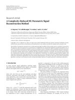
Next, as depicted in Figure 2, we extract four features
from each LF base and five features from each HF base while
only two of these two feature sets are the same. In order to
derive the discriminative features of normal and abnormal
signals, we investigate the TFD difference of the two groups.
To do so, we choose one normal and one pathological speech
and construct the Adaptive TFD of each 80 ms frame of the
signals. The sum of the TF matrices for each speech is shown
in Figure 3. We observed two major differences between the
pathological and the normal speech: (1) the pathological
signal has more transient components compared to the
normal signal, and (2) the pathological voice presents weaker
formants compared to the normal signal.
Base on the above observations, we extract the following
features from the coefficient and base vectors.
5.1. Coefficient Vectors. It is observed that the pathological
voice can be characterized by its noisy structure. The more
transients and discontinuities are present in the signal, the
more abnormality is observed in the speech. Two features are

proposed to represent this characteristic of the pathological
speech.
5.1.1. Sparsity. Sparsity of the coefficient vector distinguishes
the nonfrequent transient components of the abnormal
signals from the natural frequent components. Several
sparseness measures have been proposed in the literature. In
this paper, we use the function defined as
S
h
i
=
√
N −


N
n=1
h
i
(
n
)

/


N
n=1
h
2

i
√
N − 1
.
(15)
The above function is unity if and only if h
i
contains a
single nonzero component and is zero if and only if all the
components are equal. The sparsity measure in (15)hasbeen
used for applications such as NMF matrix decomposition
with more part-based properties [19]; however, it has never
been used for feature extraction application.
The next proposed feature differentiates the discontinu-
ity characteristics of the pathological speech from the normal
signal.
5.1.2. Sum of Derivative. We h ave
D
h
i
=
N−1

n=1
h

i
(
n
)

2
, (16)
where
h

i
(
n
)
= h
i
(
n +1
)
−h
i
(
n
)
, n
= 1, , N −1. (17)
D
h
i
captures the discontinuities and abrupt changes, which
are typical in pathological voice samples.
5.2. Base Vectors. The base vectors represent the frequency
components present in the signal. The dynamics of the voice
abnormality varies between HF and LF-bases groups. Hence,
we extracted different frequency features for each group.

5.2.1. Moments. Our observation showed that in the patho-
logical speech, the HF bases tend to have bases with energy
concentration at higher frequencies compared to the normal
signals. To discriminate this abnormality property, we extract
the first three moments of the base vectors as the features:
MO
(o)
w
i
=
M

m=1
f
o
w
i
(
m
)
, o
= 1, 2, 3 (18)
where MO
1
, MO
2
,andMO
3
are the three moments, and
M is the frequency resolution. The moment features are

extracted from HF bases; the higher are the frequency
energies, the larger will the feature values be. Although these
features are useful for distinguishing the abnormalities of
6 EURASIP Journal on Advances in Signal Processing
0.05
0.1
0.15
0.2
0.25
0.3
0.35
0.4
0.45
0.5
Normalized frequency
10 20 30 40 50 60 70 80
Time (ms)
(a) TF distribution of a normal voice with a male speaker
0.05
0.1
0.15
0.2
0.25
0.3
0.35
0.4
0.45
0.5
Normalized frequency
10 20 30 40 50 60 70 80

Time (ms)
(b) TF distribution of a pathological voice with a male speaker
Figure 3: TFD of a normal (a) and an abnormal signal (b) is constructed using adaptive TFD with Gabor atoms, 100 MP iterations and 5
MCE iterations. As evident in theses figures, the pathological signal has more transient components specially at high frequencies. In addition,
the TF of the pathological signal presents weak formants, while the normal signal has more periodicity in low frequencies, and introduces
stronger formants.
the HF components, there are not useful for representing
the abnormalities of the LF bases. The reason is that the
major frequency changes in the LF components is dominated
by the difference in pitch frequency of speech from one
speaker to another speaker, and it does not provide any
discrimination between normality or abnormality of the
speech. Two features are proposed for LF bases.
5.2.2. Sparsity. As is known in literature, it is expected to
observe periodic structures in the low frequency components
of the normal speech. Therefore, when a large amount of
scattered energy is observed in the low frequency compo-
nents, we conclude that a level of abnormality is present in
the signal. To measure this property, we propose the sparsity
of the base vectors
{w
i
}
i=1, ,M
as given below:
S
w
i
=
√

M −


M
m
=1
w
i
(
m
)

/


M
m
=1
w
2
i
√
M −1
.
(19)
For normal signals we expect to have higher sparsity fea-
tures, while pathological speech signals have lower sparsity
values.
5.2.3. Sharpness. S
w

i
measures the spread of the components
in low frequencies. In addition, we need another feature
to provide an information on the energy distribution in
frequency. Comparing the LF bases of the normal and the
pathological signals, we notice that normal signals have
strong formants; however, the pathological signals have weak
and less structured formants.
For each base vector, first we calculate the Fourier
transform as given
W
i
(
ν
)
=






M

f =1
e
−j
(
2πmν/M
)

w
i
(
m
)






.
(20)
where M is length of the base vector, and W
i
(ν) is the Fourier
transform of the base vector w
i
. Next, we perform a second
Fourier transform on the base vector, and obtain W
i
(κ)as
follows:
W
i
(
κ
)
=







M/2

ν=1
e
−j
(
2πνκ/
(
M/2
))
W
i
(
ν
)






. (21)
Finally, we sum up all the values of
|W(κ)| for κ more than
m

0
,wherem
0
is a small number:
SH
w
i
=
M/4

κ=m
0
|W
i
(
κ
)
|. (22)
In Appendix B, we demonstrate that SH
w
i
is a large value
for bases representing strong formants, such as in normal
speech, but is a small value for distorted formants, such as
in pathological speech.
5.3. Classification. As it is shown in Figure 1, once the
features are extracted, we feed them into a pattern classifier,
which consists of a training and a testing stage.
5.3.1. Training Stage. Various classifiers were used for patho-
logical voice classification [8], such as, the linear discrimi-

nant analysis, hidden Markov models, and neural networks.
In the proposed technique, we use K-means clustering as a
simple classifier.
EURASIP Journal on Advances in Signal Processing 7
f
HF
test
={f
HF
t
}
t=1, ,
T
HF
C
HF
test
={C
HF
i
}
t=1, ,
T
HF
if C
HF
t
 C
HF
abn

if C
LF
t
 C
LF
abn
min




5

i=1
( f
HF
i
(i) −C
HF
k
(i))
2
min




4

i=1

( f
LF
i
(i) −C
LF
k
(i))
2
k = 1, , K
k
= 1, , K
f
LF
test
={f
LF
t
}
t=1, ,
T
LF
C
LF
test
={C
LF
t
}
t=1, ,
T

LF
abn
HF
test
= abn
HF
test
+1
abn
LF
test
= abn
LF
test
+1
abn
HF
test
T
HF
+
abn
LF
test
T
LF
abn
>
<
norm

Th
patho
Figure 4:Theblockdiagramoftheteststage.
K-means clustering is one of the simplest unsupervised
learning algorithms. The method starts with an initial
random centroids, and it iteratively classifies a given data
set into a certain number of clusters (K) by minimizing the
squared Euclidean distance of the samples in each cluster to
the centroid of that cluster. For each cluster, the centroid is
the mean of the points in that cluster C
i
.
Since separate features are extracted for LF and HF
components, we have to train a separate classifier for each
group: C
LF
and C
HF
for LF and HF components, respectively.
Once the clusters are estimated, we count the number of
abnormality feature vectors in each cluster, and the cluster
with a majority of abnormal points is labeled as abnormal
clusters; otherwise, the cluster is labeled as normal
C
k
∈
⎧
⎪
⎨
⎪

⎩
Abnormality, if

f
C
k
abn
>α

f
C
k
n
,
Normality, if

f
C
k
abn
<α

f
C
k
n
,
(23)
where


f
C
k
abn
and

f
C
k
n
are the total number of abnormality
and normality features in the cluster C
k
,respectively.We
found the value of α equal to 1.2tobeaproperchoicefor
this threshold.
In (23), we choose the classes that represent the abnor-
mality in the speech. The equation distinguishes a cluster as
abnormal if the number of the features estimated from the
pathological voice is more than features derived from the
normal speech. The abnormality clusters are denoted as C
LF
abn
and C
HF
abn
for LF and HF groups, respectively.
5.3.2. Testing Stage. In this stage, we test the trained classifier.
For a voice sample, we find the nearest cluster to each of
its feature vectors using Euclidean distance criterion. If the

number of the feature vectors that belong to the abnormality
clusters is dominant, the voice sample is classified as a
pathological voice; otherwise, it is classified as a normal
speech.
Figure 4 demonstrates the testing stage. f
LF
Te s t
and f
HF
Te s t
feature vectors are derived from the base and coefficient
vectors in LF and HF groups, respectively. For each feature
vector, we find the closest cluster, C
k
0
,asgivenin
f
LF
t
∈ C
LF
k
0
if k
0
= min
k=1, ,K






4

i=1

f
LF
t
(
i
)
−C
LF
k
(
i
)

2
,
t
=1, , T
LF
,
f
HF
t
∈ C
HF

k
0
if k
0
= min
k=1, ,K





5

i=1

f
HF
t
(
i
)
−C
HF
k
(
i
)

2
,

t
=1, , T
HF
,
(24)
where f
LF
t
and f
HF
t
are the input feature vectors, and T
HF
and
T
LF
are the total numbers of test feature vectors for HF and
LF components, respectively.
Next, the number of all the features that belong to
abnormal and normal clusters is calculated
if C
LF
k
0
∈ C
LF
abn
=⇒ abn
LF
test

= abn
LF
test
+1,
if C
HF
k
0
∈ C
HF
abn
=⇒ abn
HF
test
= abn
HF
test
+1,
(25)
where abn
LF
test
and abn
HF
test
are the numbers of all the feature
vectors of LF and HF groups that belong to an abnormal
cluster.Thesignalisclassifiedasnormalif
L
abnormality

<Th
patho
,
(26)
where Th
patho
is the abnormality threshold, and L
abnormality
is
the number of the abnormality features in the voice sample:
L
abnormality
=

abn
LF
test
T
LF
+
abn
HF
test
T
HF

. (27)
If the criterion in (26) is not satisfied, the signal is classified
as a pathological speech.
8 EURASIP Journal on Advances in Signal Processing

5
10
15
NPE
50 100 150 200
Iteration
(a)
5
10
15
NPE
50 100 150 200
Iteration
(b)
Figure 5: The normalized projected energy (NPE) at each iteration
is plotted for one normal (a) and one pathological signal (b). As it
can be observed in this figure, most of the coherent structure of the
signal is projected before 100 iterations, and the remaining energy
is negligible.
6. Results
The proposed methodology was applied to the Massachusetts
Eye and Ear Infirmary (MEEI) voice disorders database, dis-
tributed by Kay Elemetrics Corporation [20]. The database
consists of 51 normal and 161 pathological speakers whose
disorders spanned a variety of organic, neurological, trau-
matic, and psychogenic factors. The speech signal is sampled
at 25 kHz and quantized at a resolution of 16 bits/sample. In
this paper, 25 abnormal and 25 normal signals were used to
train the classifier.
MP-TFD with Gabor atoms is estimated for each 80 ms

of the signal. Gabor atoms provide optimal TF resolution
in the TF plane and have been commonly used in MP-
TFD. To acquire the required iterations (I) in the MP
decomposition, we calculate the energy of the projected
signal at each iteration,
R
i
x, g
γ
i
 in (A.2). Figure 5 illustrates
the mean of the projected energy per iteration for one
normal and one pathological signal. As evident in this figure,
most of the coherent structure of the signal is projected
before 100 iterations. Therefore, in this paper, MP-TFD is
constructed using the first 100 iterations and the remaining
energy is ignored. As explained in Section 3.1, the Adaptive
TFD is constructed by performing MCE iterations to the
estimated MP-TFD. It can be shown that after 5 iterations,
the constructed TFD satisfies the marginal criteria in (5).
Next, we apply NMF-MD with base number of r
= 15
to each TF matrix and estimate the base and coefficient
matrices, W and H, respectively. Each base vector is catego-
rized into either LF or HF group a base vector is grouped
as LF component if its energy is concentrated more in the
frequency range of 4 kHz or less; otherwise, it is grouped
as HF component. We extract 4 features (S
h
, D

h
, S
w
, SH
w
)
from each LF base vector w and its coefficient vector h,and
5features(S
h
, D
h
, MO
(1)
w
, MO
(2)
w
, MO
(3)
w
)fromeachHFbase
S
h
D
h
S
w
SH
w
S

h
D
h
MO
(1)
w
MO
(2)
w
MO
(3)
w
LF features HF features
Feature importance
Figure 6: The relative height of each feature represents the relative
importance of the feature compared to the other features.
vector and its coefficient vector. In order to obtain the role
of each feature in the classification accuracy, we calculate the
P-value of each feature using the Student’s t-test. The feature
with the smallest P-value plays the most important role in
the classification accuracy. Figure 6 demonstrates the relative
importance of each 9 features. As shown in this figure, D
h
and SH
w
from LF features, and S
h
, MO
(2)
w

and MO
(3)
w
from
HF features play the most significant role in the classification
accuracy.
Finally, we apply the K-means clustering to the logarithm
of the derived feature vectors, and define the abnormality
clusters. Figures 7 illustrates the application of the proposed
methodology for a pathological voice sample which is shown
in Figure 7(a). As explained in Section 5.3, the test procedure
determines the feature vectors that belong to the abnor-
mality clusters. We use the base and coefficient matrices,
W
abn
and H
abn
, corresponding to the abnormality feature
vectors to reconstruct the abnormality TF matrix, V
abn
,as
V
abn
= W
abn
H
abn
. Figure 7(b) depicts the reconstructed TF
matrix. As it is expected, the proposed method successfully
distinguishes transients, high frequency components, and

week formants as abnormality.
In the test stage, the trained classifier is used to calculate
the measure of abnormality (L
abnormality
in (27)) for each
voice sample. Figure 8 shows the abnormality measure for
51 normal and 161 pathological speech signals in MEEI
database. As evident in this figure, the pathological samples
have higher abnormality measure compared to the normal
samples. Each signal is classified as normal if its abnormality
measure is smaller than a threshold (Th
patho
in (26));
otherwise it is classified as pathological. In order to find
the abnormality threshold, receiver operating curves (ROCs)
of L
abnormality
are computed with the area under the curve
indicating relative abnormality detection (Figure 9). Based
on the ROC, the cut point of 0.59 is chosen as the
abnormality threshold (Th
patho
= 0.59). Ta bl e 1 shows the
accuracy of the classifier. From the table, it can be observed
that out of 51 normal signals, 50 were classified as normal,
and only 1 was misclassified as pathological. Also, the table
shows that out of 161 pathological signals, 159 were classified
EURASIP Journal on Advances in Signal Processing 9
0.05
0.1

0.15
0.2
0.25
0.3
0.35
0.4
0.45
0.5
Normalized frequency
10 20 30 40 50 60 70 80
Time (ms)
(a) TFD of a pathological speech
0.05
0.1
0.15
0.2
0.25
0.3
0.35
0.4
0.45
0.5
Normalized frequency
0.01 0.02 0.03 0.04 0.05 0.06 0.07 0.08
Time (ms)
(b) TFD of the estimated abnormality
Figure 7: The classifier of Figure 4 is applied to the TF matrix of a
pathological speech shown in (a), and the estimated abnormality TF
matrix is shown in (b) . As evident in this figure, the abnormality
components are mainly transients, high frequency components, and

week formants.
as pathological and only 2 were misclassified as normal.
The total classification accuracy is 98.6%. As it can be
concluded from the result, the extracted features successfully
discriminate the abnormality region in the speech.
In Figure 9 and Tab l e 1, we utilized MD with decomposi-
tion order (r) of 15. We repeated the proposed method using
different decomposition orders. Our experiment showed
that the decomposition order of 5 and higher is suitable
for our application. Ta bl e 2 shows the P-values of three
decomposition orders obtained with the Student’s t-test.
As explained in Section 2, our proposed feature extrac-
tion methodology performs a longer term modeling com-
pared to the current methods. The pathological speech
classification is conventionally performed on 10–30 ms of
signal. At sampling frequency of 8 kHz, the number of
sample is 80–240 samples per segment. In this paper, we
0
2
4
6
8
Abnormality measure
50 100 150
Voice sample
Pathological
Normal
Figure 8: For each voice sample, the number of the feature
vectors that belong to an abnormality cluster is calculated, and the
abnormality measure is calculated as the ratio of the total number of

the abnormal feature vectors to the total number of feature vectors
in the voice sample.
0
0.2
0.4
0.6
0.8
1
Senstivity
00.20.40.60.81
1-Specificity
ROC curve
Figure 9: Receiver operating curve for the pathological voice classi-
fication is plotted. In this analysis, pathological speech is considered
negative, and normal is considered positive. The area under the
ROC is 0.999, and the maximum sensitivity for pathological speech
detection while preserving 100% specificity is 98.1%.
use 80 ms of speech at sampling frequency of 25 kHz. As
a result, we are working with 2048 samples/frame which
is 10 times the conventional length. The results shown in
this section demonstrate that the proposed methodology
successfully discriminates the pathological characteristics
of the speech. In addition to the high accuracy rate, the
advantage of our proposed methodology can be concluded
in 3 points. (1) By performing MP on the speech signal,
we project the most coherent structure of the signal. The
10 EURASIP Journal on Advances in Signal Processing
Table 1: Classification result.
Classes Normal Abnormal Total
Normal 50 1 51

Pathological 2 159 161
Normal 98.0% 2.0% 100%
Pathological 1.2% 98.8% 100%
Table 2: P -value of the classifiers obtained with three different
decomposition orders.
Decomposition order (r) 5 10 15
P-value 3 ×10
−10
1 ×10
−11
1 ×10
−13
remaining part represents the random noise presented in the
signal. Hence, we perform an automatically denoising on
the signal which allows the technique to be practical in the
low SNR speech signals. (2) In this method, we reconstruct
the TF matrix of the abnormality part of the signal, and we
estimate the amount of abnormality in the speech signal.
The reconstructed TF matrix and the abnormality measure
have potential to be used as a patients’ progress measure
over the course of voice therapy. (3) In this work, we use a
very simple classifier rather than a complex classifier, such as
hidden Markov models or neural networks.
7. Conclusion
TF analysis are effective for revealing non-stationary aspects
of signals such as trends, discontinuities, and repeated
patterns where other signal processing approaches fail or
are not as effective;however,mostoftheTFanalysis
are restricted to visualization of TFDs and do not focus
on quantification or parametrization that are essential for

feature analysis and pattern classification.
In this paper, we presented a joint TF and MD feature
extraction approach for pathological voice classification. The
proposed methodology extracts meaningful speech features
that are difficult to be captured by other means. TF features
are extracted from a positive TFD that satisfies the marginal
conditions and can be considered as a true joint distribution
oftimeandfrequency.TheutilizedTFDisasegmentfreeTF
approach, and it provides a high-resolution and cross-term
free TFD.
The TF matrix was decomposed into its base (spectral)
and coefficient (temporal) vectors using nonnegative matrix
factorization (NMF) method. Four features were extracted
from the components with low frequency structure, and five
features were derived from the bases with high frequency
composition. The features were extracted from the decom-
posed vectors based on the spectral and temporal character-
istics of the normal and pathological signals. In this study,
we performed K-means clustering to the proposed feature
vectors, and we achieved an accuracy rate of 98.6% for the
MEEI voice disorders database, including 161 pathological
and 51 normal speakers.
Appendices
A. Matching Pursuit TFD
Matching pursuit (MP) was proposed by Mallat and Zhang
[21] in 1993 to decompose a signal into Gabor atoms, g
γ
i
,
with a wide variety of modulated frequency ( f

i
)andphase
(φ
i
), time shift (p
i
)andduration(s
i
) as shown in
g
γ
i
(
t
)
=
1
√
s
i
g

t − p
i
s
i

exp

j


2

πf
i
t + φ
i

,
(A.1)
where γ
i
represents the set of parameters (s
i
, p
i
, f
i
, φ
i
). The
MP dictionary is consisted of Gabor atoms with durations
(s
i
) varying from 2 samples to N (length of the signal x(t)),
and it therefore is a very flexible technique for non-stationary
signal representation. At each iteration, the MP algorithm
chooses the Gabor atom that best fits to the input signal.
Therefore, after I iterations, MP procedure chooses the
Gabor atoms that best fit to the signal structure without any

preassumption about the signal’s stationarity. Components
with long stationarity properties will be represented by long
Gabor atoms, and transients will be characterized by short
Gabor atoms.
At each iteration, MP projects the signal into a set of TF
atomsasfollows:
x
(
t
)
=
I−1

i=0

R
i
x
, g
γ
i

g
γ
i
(
t
)
+ R
I

x
,(A.2)
where
R
i
x
, g
γ
i
 is the expansion coefficient on atom g
γ
i
(t),
and R
I
x
is the decomposition residue after I decomposition.
At this stage, the selected components represent coherent
structures and the residue represents incoherent structures
in the signal. The residue may be assumed to be due to
random noise, since it does not show any TF localization.
Therefore, the decomposition residue in (A.2)isignored,and
the Wigner-Ville distribution (WVD) of each I components
is added in the following:

V

t, f

=

I−1

i=0




R
i
x
, g
γ
i




2
Wg
γ
i

t, f

,(A.3)
where Wg
γ
i
(t, f ) is the WVD of the Gabor atom g
γ

i
(t),
and

V(t, f ) is called the MP-TFD. Wigner distribution is a
powerful TF representation; however when more than one
component is present in the signal, the TF resolution will be
confounded by cross-terms. Nevertheless, when we apply the
Wigner distribution to single components and add them up,
the summation will be a cross-term free TFD.
EURASIP Journal on Advances in Signal Processing 11
B. Analysis of sharpness feature
In order to demonstrate the behavior of feature SH
w
,we
assume that the base vector, w
i
, has two components at
frequencies samples m
1
and m
2
with energies of α and β,
respectively
w
i
(
m
)
= αδ

(
m − m
1
)
+ βδ
(
m
−m
2
)
,
(B.1)
|W(ν)|(21) is calculated as
|W
(
ν
)
|=

α
2
+ β
2
+2αβ cos
(
2π
(
m
1
−m

2
)
ν
)
. (B.2)
|W(ν)| is independent to the parameter ν only when m
1
≈
m
2
, or when the energy ratio of the components in (B.1)is
too small (either β/α
≈ 0orα/β ≈ 0). In this case, when we
calculate the Fourier transform of
|W(ν)| as shown in (21),
|W(κ)| is non-zero only at small values of κ (say κ<m
0
,
where m
0
is a small number). Hence, SH
w
i
as it is calculated
in (22) results in a small feature. From the other side,
|W(ν)|
is dependent on the parameter ν when both the components
in (B.1) are strong (β/α
≈ R, R
/

=0). In this case, the Fourier
transform of
|W(ν)| is not negligible at κ>m
0
,andSH
w
i
results in lager values.
From the above explanation, we conclude that the small
values of SH
w
i
represent pathological formants, in which the
components’ energies are very small compared to the energy
of the main frequency (β/α
≈ 0orα/β ≈ 0), and the large
values of SH
w
i
show the strong formants in speech (β/α ≈
R, R
/
=0).
References
[1] R. T. Sataloff, Professional Voice: The Science and Art of Clinical
Care, Raven Press, New York, NY, USA, 1991.
[2] P. Carding and A. Wade, “Managing dysphonia caused by
misuse and abuse,” British Medical Journal, vol. 321, pp. 1544–
1545, 2000.
[3] E. J. Wallen and J. H. L. Hansen, “A screening test for speech

pathology assessment using objective quality measures,” in
Proceedings of International Conference on Spoken Language
Processing (ICSLP ’96) , vol. 2, pp. 776–779, Philadelphia, Pa,
USA, October 1996.
[4]R.J.Moran,R.B.Reilly,P.deChazal,andP.D.Lacy,
“Telephony-based voice pathology assessment using auto-
mated speech analysis,” IEEE Transactions on Biomedical
Engineering, vol. 53, no. 3, pp. 468–477, 2006.
[5] T. Ananthakrishna, K. Shama, and U. C. Niranjan, “k-means
nearest neighbor classifier for voice pathology,” in Proceedings
of the IEEE India Conference INDICON, pp. 352–354, Indian
Institute of Technology, Kharagpur, India, 2004.
[6] A. A. Dibazar, S. Narayanan, and T. W. Berger, “Feature
analysis for automatic detection of pathological speech,” in
Proceedings of Annual International Conference of the IEEE
Engineering in Medicine and Biology (EMBS ’02), vol. 1, pp.
182–183, Houston, Tex, USA, 2002.
[7] J. I. Godino-Llorente and P. G
´
omez-Vilda, “Automatic detec-
tion of voice impairments by means of short-term cepstral
parameters and neural network based detectors,” IEEE Trans-
actions on Biomedical Engineering, vol. 51, no. 2, pp. 380–384,
2004.
[8] A. Gelzinis, A. Verikas, and M. Bacauskiene, “Automated
speech analysis applied to laryngeal disease categorization,”
Computer Methods and Programs in Biomedicine, vol. 91, no.
1, pp. 36–47, 2008.
[9] N. S
´

aenz-Lech
´
on, J. I. Godino-Llorente, V. Osma-Ruiz, and P.
G
´
omez-Vilda, “Methodological issues in the development of
automatic systems for voice pathology detection,” Biomedical
Signal Processing and Control, vol. 1, no. 2, pp. 120–128, 2006.
[10] V. Parsa and D. G. Jamieson, “Identification of pathological
voices using glottal noise measures,” Journal of Speech, Lan-
guage, and Hearing Research, vol. 43, no. 2, pp. 469–485, 2000.
[11] K. Umapathy, S. Krishnan, V. Parsa, and D. G. Jamieson,
“Discrimination of pathological voices using a time-frequency
approach,” IEEE Transactions on Biomedical Engineering, vol.
52, no. 3, pp. 421–430, 2005.
[12] F. Auger and P. Flandrin, “Improving the readability of time-
frequency and time-scale representations by the reassignment
method,” IEEE Transactions on Signal Processing, vol. 43, no. 5,
pp. 1068–1089, 1995.
[13] L. Cohen and T. E. Posch, “Positive time-frequency distribu-
tion functions,” IEEE Transactions on Acoustics, Speech, and
Signal Processing, vol. 33, no. 1, pp. 31–38, 1985.
[14] S. Krishnan, R. M. Rangayyan, G. D. Bell, and C. B. Frank,
“Adaptive time-frequency analysis of knee joint vibroarthro-
graphic signals for noninvasive screening of articular cartilage
pathology,” IEEE Transactions on Biomedical Engineering, vol.
47, no. 6, pp. 773–783, 2000.
[15] B. Ghoraani and S. Krishnan, “Quantification and localiza-
tion of features in time-frequency plane,” in Proceedings of
Canadian Conference on Electrical and Computer Engineering

(CCECE ’08), pp. 1207–1210, May 2008.
[16] D. D. Lee and H. S. Seung, “Algorithms for non-negative
matrix factorization,” in Proceedings of the Conference on
Advances in Neural Information Processing Systems (NIPS ’01),
pp. 556–562, 2001.
[17] M.W.Berry,M.Browne,A.N.Langville,V.P.Pauca,andR.
J. Plemmons, “Algorithms and applications for approximate
nonnegative matrix factorization,” Computational Statistics
and Data Analysis, vol. 52, no. 1, pp. 155–173, 2007.
[18] C J. Lin, “Projected gradient methods for nonnegative matrix
factorization,” Neural Computation, vol. 19, no. 10, pp. 2756–
2779, 2007.
[19] P. O. Hoyer, “Non-negative matrix factorization with sparse-
ness constraints,” Journal of Machine Learning Research, vol. 5,
pp. 1457–1469, 2004.
[20] M. Eye and E. Infirmary, Voice Disorders Database, Version
1.03, Kay Elemetrics Corporation, Lincoln Park, NJ, USA,
1994.
[21] S. G. Mallat and Z. Zhang, “Matching pursuits with time-
frequency dictionaries,” IEEE Transactions on Signal Process-
ing, vol. 41, no. 12, pp. 3397–3415, 1993.