Báo cáo hóa học: "Research Article A Rules-Based Approach for Configuring Chains of Classifiers in Real-Time Stream Mining Systems Brian Foo and Mihaela van der Schaar" pot

Hindawi Publishing Corporation
EURASIP Journal on Advances in Signal Processing
Volume 2009, Article ID 975640, 17 pages
doi:10.1155/2009/975640
Research Article
A Rules-Based Approach for Configuring Chains of Classifiers in
Real-Time Stream Mining Systems
Brian Foo and Mihaela van der Schaar
Department of Electrical Engineering, University of California Los Angeles (UCLA), 66-147E Engineering IV Building,
420 Westwood Plaza, Los Angeles, CA 90095, USA
Correspondence should be addressed to Brian Foo,
Received 20 November 2008; Revised 8 April 2009; Accepted 9 June 2009
Recommended by Gloria Menegaz
Networks of classifiers can offer improved accuracy and scalability over single classifiers by utilizing distributed processing
resources and analytics. However, they also pose a unique combination of challenges. First, classifiers may be located across
different sites that are willing to cooperate to provide services, but are unwilling to reveal proprietary information about their
analytics, or are unable to exchange their analytics due to the high transmission overheads involved. Furthermore, processing
of voluminous stream data across sites often requires load shedding approaches, which can lead to suboptimal classification
performance. Finally, real stream mining systems often exhibit dynamic behavior and thus necessitate frequent reconfiguration of
classifier elements to ensure acceptable end-to-end performance and delay under resource constraints. Under such informational
constraints, resource constraints, and unpredictable dynamics, utilizing a single, fixed algorithm for reconfiguring classifiers can
often lead to poor performance. In this paper, we propose a new optimization framework aimed at developing rules for choosing
algorithms to reconfigure the classifier system under such conditions. We provide an adaptive, Markov model-based solution for
learning the optimal rule when stream dynamics are initially unknown. Furthermore, we discuss how rules can be decomposed
across multiple sites and propose a method for evolving new rules from a set of existing rules. Simulation results are presented for
a speech classification system to highlight the advantages of using the rules-based framework to cope with stream dynamics.
Copyright © 2009 B. Foo and M. van der Schaar. This is an open access article distributed under the Creative Commons
Attribution License, which permits unrestricted use, distribution, and reproduction in any medium, provided the original work is
properly cited.
1. Introduction
A variety of real-time applications require complex topolo-

gies of operators to perform classification, filtering, aggre-
gation, and correlation over high-volume, continuous data
streams [1–7]. Due to the high computational burden of
analyzing such streams, distributed stream mining systems
have been recently developed. It has been shown that
distributed stream mining systems transcend the scalability,
reliability, and performance objectives of large-scale, real-
time stream mining systems [5, 7–9]. In particular, many
mining applications implement topologies of classifiers to
jointly accomplish a complex classification task [10, 11].
Such structures enable the application to leverage computa-
tional resources and analytics across different sites to provide
dynamic filtering and successive identification of stream
data.
Nevertheless, several key challenges remain for config-
uring networks of classifiers in distributed stream mining
systems. First, real-time stream mining applications must
cope effectively with system overload due to large data
volumes, or limited system resources, while maintain-
ing high classification performance (i.e., utility). A novel
methodology was introduced recently for configuring the
operating point (e.g., threshold) of each classifier based on
its performance, as well as its output data rate, such that
the joint configurations meet the resource constraints at all
downstream classifiers in the topology while maximizing
detection rate [11]. In general, such operation points exist for
a majority of classification schemes, such as support vector
machines, k-Nearest neighbors, Maximum Likelihood, and
Random Decision Trees. While this methodology performs
well when the relationships between classifier analytics are

known (e.g., the exclusivity principle for filtering subset data
2 EURASIP Journal on Advances in Signal Processing
Proposed framework
Goal:
maximize current
performance
Goal:
maximize expected
performance under
dynamics
Input stream Filtered stream
Classifiers
Single algorithm
Reconfiguration
Estimation
Prior approaches
Input stream
Filtered stream
Classifiers
Choosing from
multiple algorithms
Adapting and
evolving rules
Reconfiguration
Constructing
system states
Estimation
Modelin
g
of dynamics

Decision
making
Stream APP π,utilityQ
Stream APP π,utilityQ
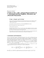
Figure 1: Comparison of prior approaches and the proposed rules-based framework.
from the previous classifier [11]), joint optimization between
autonomous sites can be a very difficult problem, since the
analytics used to perform successive classification/filtering
may be physically distributed across sites owned by different
companies [7, 12]. These analytics may have complex rela-
tionships and often cannot be unified into a single repository
due to legal, proprietary or technical restrictions [13, 14].
Second, data streams often have time-varying rates and char-
acteristics, and thus, they require frequent reconfiguration to
ensure acceptable classification performance. In particular,
many existing algorithms optimally configure classifiers
under fixed stream characteristics [13, 15]. However, some
algorithms can perform poorly when stream characteristics
are highly time-varying. Hence, it becomes important to
design rules or guidelines to determine for each classifier the
best algorithm to use for reconfiguration at any given time,
based on its short-term as well as long-term effects on future
performance.
Inthispaper,weintroduceanovelrules-based framework
for configuring networks of classifiers in informationally
distributed and dynamic environments. A rule acts as an
instruction that determines for different stream characteris-
tics, the proper algorithm to use, for classifier reconfigura-
tion. We focus on a chain of binary classifiers as our main
application [4], since chains of classifiers are easier to analyze,

while offering flexibility in terms of configurations that can
affect both the overall quality of classification as well as the
end-to-end processing delay. Figure 1 depicts the proposed
framework compared to prior approaches for reconfiguring
chains of classifiers. The main features are highlighted as
follows.
(i) Estimation. Important local information, such as the
estimated a priori probabilities (APP) of positive data from
the input stream at each classifier and processing resource
constraints, is gathered to determine the utility of the stream
processing system. In our prior work, we introduced a
method for distributed information gathering, where each
classifier summarizes its local observations using several
scalar values [13]. The values can be exchanged between
nodes in order to obtain an accurate estimate of the overall
stream processing utility, while keeping the communications
overhead low and maintaining a high level of information
privacy across sites.
(ii) Reconfiguration. Classifier reconfiguration can be per-
formed by using an algorithm that analytically maximizes the
stream processing utility based on the processing rate, accu-
racy, and delay. Note that while, in some cases, a centralized
scheme can be used to determine the optimal configuration
[11], in informationally distributed environments, it is often
impossible to determine the performance of an algorithm
until sufficient time is given to estimate the accuracy/delay
of the processed data [13]. Such environments require the
use of randomized or iterative algorithms that converge to
the optimal configuration over time. However, when the
stream is dynamic, it often does not make sense to use an

algorithm that configures for the current time interval, since
stream characteristics may have changed during the next
time interval. Hence, having multiple algorithms available
enables us to choose the optimal algorithm based on the
expected stream behavior in future time intervals.
(iii) Modeling of Dynamics. To determine the optimal algo-
rithm for reconfiguration, it is necessary to have a model of
EURASIP Journal on Advances in Signal Processing 3
stream dynamics. Stream dynamics affect the APP of positive
data arriving at each classifier, which in turn affects each
classifier’s local utility function. In our work, we define a
system state to be a quantized value over each classifier’s
local utility values as well as the overall stream processing
utility. We propose a Markov-based approach to model
state transitions over time as a function of the previous
state visited and algorithm used. This model enables us to
choose the algorithm that leads to the best expected system
performance in each system state.
(iv) Rules-Based Decision-Making. We introduce the concept
of rules, where a rule determines the proper algorithm to
apply for system reconfiguration in each state. We provide an
adaptive solution for using rules when stream characteristics
are initially unknown. Each rule is played with a different
probability, and the probability distribution is adapted to
ensure probabilistic convergence to an optimal steady state
rule. Furthermore, we provide an efficiency bound on the
performance of the convergent rule when a limited number
of iterations are used to estimate stream dynamics (i.e.,
imperfect estimation). As an extension, we also provide an
evolutionary approach, where a new rule is generated from

a set of old rules based on the best expected utility in the
following time interval based on modeled dynamics. Finally,
we discuss conditions under which a large set of rules can be
decomposed into small sets of local rules across individual
classifier sites, which can then make autonomous decisions
about their locally utilized algorithms.
While dynamic, resource-constrained, and distributed
classification is an application that very well highlights
the merits of our approach, we note that the framework
developed in this paper can also be applied to any application
that meets the following two criteria: (a) the utility can be
measured and estimated by the system during any given
time interval, but (b) the system cannot directly reconfig-
ure and reoptimize due to unknown dynamics in system
resource availabilities and application data characteristics.
Importantly, in contrast to existing works that develop
solutions for specific application domains such as optimizing
classifier trees [16] or resource-constrained/delay-sensitive
data processing [17], we are proposing a method that
encapsulates such existing algorithms and determines rules
on when to best apply them based on system and application
dynamics.
This paper is organized as follows. In Section 2,we
review several related works that address various challenges
in distributed, resource-constrained stream mining systems,
and decision-making in dynamic environments. In Section 3,
we introduce the application of interest, which is optimizing
distributed classifier chains, and propose a delay-sensitive
utility function. We also discuss a distributed information
gathering approach to estimate the utility when each site is

unwilling to share proprietary data. In Section 4, we intro-
duce the rules-based framework for choosing algorithms to
apply under different system conditions. Extensions to the
rules-based framework, such as the decomposition of rules
across distributed classifier sites and evolving a new rule
from existing rules, are discussed in Section 5. Simulation
results from a speech classification application are given in
Section 6, and conclusions in Section 7.
2. Review of Existing Works
2.1. Resource-Constrained Classification. Various works in
resource-constrained stream mining deal with both value-
independent and value-dependent load shedding schemes.
Value independent (or probabilistic) load shedding solutions
[17–22] perform well for simple data management jobs
such as aggregation, for which the quality depends only
on the sample size. However, this approach is suboptimal
for applications where the quality is value-dependent, such
as the confidence level of data in classification. A value-
dependent load shedding approach is given in [11, 15]for
chains of binary filtering classifiers, where each classifier
configures its operating point (e.g., threshold) based on the
quality of classification as well as the resource availability
across utilized processing nodes. However, in order to
analytically optimize the quality of joint classification, strong
assumptions about the relations between classifiers are often
required (e.g., exclusivity [11], where each chained classifier
filters out a subset of data from the previous classifier). Such
assumptions about classifier relationships may not be valid
when each classifier is independently trained and placed on
different sites owned by different companies.

A recent work that considers stream dynamics involves
intelligent load shedding for a classifier [23], where the load
shedder attempts to maximize certain Quality of Decision
(QoD) measures based on the predicted distribution of
feature values in future time units. However, this work
focuses mainly on load shedding for a single classifier rather
than a distributed network of classifiers. Without a joint
consideration of resource constraints and effects on feature
values at downstream classifiers, the quality of classification
can suffer, and the end-to-end processing delay can become
intolerable for real-time applications [24, 25].
Finally, in our prior work [13], we proposed a model-
free experimentation solution to maximize the performance
of a delay-sensitive stream mining application using a
chain of resource-constrained classifiers. (We provide a
brief tutorial on delay-sensitive stream mining with a chain
of classifiers in Section 3.) We proved that this solution
converged to the optimal configuration for static streams,
even when the relationships between individual classifier
analytics are unknown. However, the experimentation solu-
tion could not provide any performance guarantees for
dynamic streams. Importantly, in the above works, dynamics
and information-decentralization have been addressed in
isolation for resource-constrained classification, but there has
not been an integrated framework to address these challenges
jointly.
2.2. Markov Decision Process versus Rules-Based Decision
Making. In addition to distributed stream mining, related
works exist for decision-making in dynamic environments.
A widely used framework for optimizing the performance

4 EURASIP Journal on Advances in Signal Processing
of dynamic systems is the Markov decision process (MDP)
[26], where a Markov model is used for state transitions
as a function of the previous state and action (e.g.,
configuration) taken. In an MDP framework, there exists
an optimal policy (i.e., a function mapping states to
actions) that maximizes an expected value function,which
is often given as the sum of discounted future rewards
(e.g., expected utilities at future time intervals). When
state transition probabilities are unknown, reinforcement
learning techniques can be applied to determine the optimal
policy, which involves a delicate balance between exploitation
(playing the action that gives the highest estimated value)
and exploration (playing an action of suboptimal value)
[27].
While our rules-based framework is derived from the
MDP framework (e.g., rules map states to algorithms while
policies map states to actions), there is a key difference
between traditional MDP-based approaches and our pro-
posed rules-based approach. Unlike the MDP framework,
where actions must be specified by quantized (discrete)
configurations, algorithms are explicitly designed to perform
iterative optimization over previous configurations [28].
Hence, their outputs are not limited to a discrete set of
configurations/actions, but rather converge to a locally or
globally optimal configuration over the real (continuous)
space of configurations. Furthermore, algorithms avoid the
complication involving how the configurations (actions)
should be quantized in dynamic environments, for example,
when stream characteristics change over time.

Finally, there have been recent advances in collaborative
multiagent learning between distributed sites related to our
proposed work. For instance, the idea of using a playbook
to select different rules or strategies and reinforcing these
rules/strategies with different weights based on their perfor-
mances, is proposed in [29]. However, while the playbook
proposed in [29] is problem specific, we envision a broader
set of rules capable of selecting optimization algorithms with
inherent analytical properties leading to utility maximization
of not only stream processing but also distributed systems
in general. Furthermore, our aim is to construct a purely
automated framework for both information gathering and
distributed decision making, without requiring supervision,
as supervision may not be possible across autonomous sites
or can lead to high operational costs.
3. Background on Binary Classifier Chains
3.1. Characterizing Binary Classifiers and Classifier Chains. A
binary classifier partitions input data objects into two classes,
a “yes” class H and a “no” class
H. A binary classifier chain is
a special case of a binary classifier tree, where multiple binary
classifiers are used to detect the intersection of multiple
classes of interest. In particular, the outputs stream data
objects (SDOs); the “yes” class of a classifier, are fed as inputs
to the successive classifier in the chain [11], such that the
entire chain acts as a serial concatenation of data filters. For
simplicity of notation, we index each binary classifier in the
chain by v
i
, i = 1, , I, in the order that it processes an input

stream, as shown in Figure 2. Data objects that are classified
as “no” are dropped from the stream.
Given the ground truth X
i
for an input SDO to classifier
v
i
, denote the classification decision on the SDO by

X
i
.The
proportion of correctly forwarded samples is captured by
the probability of detection P
D
i
= Pr{

X
i
∈ H
i
| X
i
∈ H
i
},
and the proportion of incorrectly forwarded samples is
captured by the probability of false alarm P
F

i
= Pr{

X
i
∈
H
i
| X
i
/
∈H
i
}. Each classifier v
i
can be characterized by a
detection-error-tradeoff (DET) curve or a curve that maps
the false alarm configuration P
F
i
to a probability of detection
P
D
i
[30, 31]. For instance, a DET curve can be mapped out by
different thresholds on the output scores of a support vector
machine [32]. A typical DET curve is shown in Figure 3.
Due to the functional mapping from false alarm to detection
probabilities and also to maintain a representation that can
be generalized over many types of classifiers, we denote the

configuration of each classifier by its false alarm probability
P
F
i
. The vector of false alarm configurations for the entire
chain is denoted P
F
.
3.2. A Utility Function for a Chain of Classifiers. The goal
of a stream processing application is to maximize not only
the amount of processed data (the throughput), but also
the amount of data that is correctly processed by each
classifier (the goodput). However, increasing the throughput
also leads to an increased load on the system, which increases
the end-to-end delay for the stream. We can determine
the performance and delay based on the following metrics.
Suppose that the input stream to classifier v
i
has apriori
probability (APP) π
i
of being in the positive class. The
probability of labeling an SDO as positive can be given by

i
= π
i
P
D
i

+
(
1 −π
i
)
P
F
i
. (1)
The probability of correctly labeling an SDO as positive can
be given by
℘
i
= π
i
P
D
i
. (2)
For a chain of classifiers as shown in Figure 2, the end-to-end
cost can be given by
C
=
(
π
−℘
)
+ θ
(


−℘
)
= π −
n

i=1
℘
i
+ θ
⎛
⎝
n

i=1

i
−
n

i=1
℘
i
⎞
⎠
,
(3)
where π indicates the true APP of input data that belongs to
the intersection of all positive classes of the classifiers, and θ
specifies the cost of false positives relative to true positives.
Since π depends only on the stream characteristics, we can

regard it as constant and remove it from the cost function,
invert it, and produce a utility function: F
=

n
i=1
℘
i
−
θ(

n
i
=1

i
−

n
i
=1
℘
i
)[13, 15]. Note that

n
i
=1

i

is simply the
total fraction of stream data forwarded across the entire
chain.

n
i=1
℘
i
=

n
i=1
π
i
P
D
i
, on the other hand, is the fraction
of data out of the entire stream that is correctly forwarded
across the entire chain, which is calculated by the probability
EURASIP Journal on Advances in Signal Processing 5
Table 1: Summary of parameter types and a few examples.
Type of parameter for v
i
Description Examples
Static parameters Fixed parameters, exchanged during initialization π
Observed parameters Can be measured by the last classifier v
n
D
Exchanged parameters Traded with other classifiers

℘
i
, 
i
Configurable parameters Configured by classifier v
i
P
F
i
Forwarded Forwarded
Forwarded
Dropped Dropped Dropped
Source
stream
Processed
stream
v
1
π
1
P
D
1
(1 − π
1
)P
F
1
v
2

π
2
P
D
2
(1 − π
2
)P
F
2
v
n
π
n
P
D
n
(1 −π
n
)P
F
n
Figure 2: Classifier chain with probabilities labeled on each edge.
of detection by each classifier, times the conditional APP of
positive data at the input of each classifier v
i
.
To factor in the delay, we consider an end-to-end
processing delay penalty G(D)
= e

−ϕD
,whereϕ reflects the
application’s delay sensitivity [24, 25], with large ϕ indicating
that the application is highly delay sensitive, and small ϕ
indicating that the delay on processed data is unimportant.
Note that this function not only has an important meaning
as a discount factor in game theoretic literature [26] but also
can also be analytically derived by modeling each classifier
as an M/M/1 queuing facility often used for networks and
distributed stream processing systems [33, 34]. Denote the
total SDO input rate and the processing rate for each
classifier v
i
,byλ
i
and μ
i
, respectively. Note furthermore from
(1) that each classifier acts as a filter that drops each SDO
with i.i.d. probability 1
−
i
, and forwards the SDO with i.i.d.
probability 
i
to the next-hop classifier, based on its operating
point on the DET curve. The resulting output to each next-
hop classifier is also given by a Poisson process [35], where
the arrival rate of input data to classifier v
i

is given by
λ
i
= λ
0

i−1
j
=1

j
. Because the output of an M/M/1system
has i.i.d. interarrival times, the delays for each classifier in
a classifier system, given the arrival and service rates, are
also independent [36]. Hence, the expected delay penalty
G(D) for the entire chain can be calculated from the moment
generating function [37]:
E
[
G
(
D
)
]
= Φ
D

−
ϕ


=
n

i=1

μ
i
−λ
i
μ
i
−λ
i
+ ϕ

. (4)
In order to combine the two different objectives (accuracy
and delay), we construct a single objective function F
·
G(D), based on the concept of fairness implemented by
the Nash product [38]. (The generalized Nash product
provides a tradeoff between misclassification cost [15, 39]
and delay depending on the exponent attached to each term
F
α
and H(D)
(
1
−α
)

,respectively.Inpractice,weobserved
through simulations that, for the considered applications, an
equal weight α
= 0.5 provided the best tradeoff between
classification accuracy and delay.) The overall utility of real-
time stream processing is therefore
max
P
F
∀v
i
∈V
Q

P
F

=
max
P
F
G
(
D
)
⎛
⎝
n

i=1

℘
i
−θ
⎛
⎝
n

i=1

i
−
n

i=1
℘
i
⎞
⎠
⎞
⎠
s.t. 0 ≤ P
F
≤ 1.
(5)
3.3. Information-Distributed Estimation of Stream Processing
Utility. Note that while classifiers may be willing to provide
information about P
F
i
and P

D
i
, the conditional APP π
i
at
every classifier v
i
is, in general, a complicated function of
the false alarm probabilities of all previous classifiers, that is,
π
i
= π
i
(P
F
j
)
j<i
. This is because setting different thresholds for
the false alarm probabilities at previous classifiers will affect
the incoming source distribution to classifier v
i
.Onewayto
visualize this effect is to consider a Gaussian mixture model
operated on by a chain of 2 linear classifiers, where changing
the threshold of the first classifier will affect the positive and
negative data distribution of the second classifier. However,
because analytics trained across different sites may not
obey simple relationships (e.g., subsets), constructing a joint
classification model is very difficult if sites do not share

their analytics. Due to legal and proprietary restrictions, it
can be assumed that, in practice, the joint model cannot
be constructed, and hence the objective function Q(P
F
)is
unknown.
While the precise form of Q(P
F
) is unknown and is
most likely changing due to stream dynamics, the utility
can still be estimated over a short time interval if classifier
configurations are held fixed over the length of the interval.
This is discussed in more detail in our prior work and
summarized in Figure 4. First, the average service rate μ
i
is fixed (static ) for each classifier and can be exchanged
with other classifiers upon system initialization. Second,
the arrival rate into classifier v
i
, λ
i
, can be obtained by
simply measuring (or observing) the number of SDOs in the
input stream. Finally, the goodput and throughput ratios
℘
i
and 
i
are functions of the configuration P
F

i
and the
6 EURASIP Journal on Advances in Signal Processing
0
0.2
0.4
0.6
0.8
1
P
d
00.20.40.60.81
P
f
DET curve for a basketball image classifier
Figure 3: The DET curve for an image classifier used to detect
basketball images [40].
APP. The APP can be estimated from the input stream
using maximum a priori (MAP) schemes. Consequently,
every parameter in (5) can be easily estimated based on
some locally observable data. By exchanging these locally
obtained parameters and configurations across all classifiers,
each classifier can then estimate the overall stream processing
utility. Tab le 1 summarizes the various parameter types, their
descriptions, and examples in our problem.
4. A Rules-Based Framework for
Choosing Algorithms
4.1. States, Algorithms, and Rules. Now that we have dis-
cussed the estimation portion of our framework (Figure 1),
we move to discuss the proposed decision-making process

in dynamic environments. We introduce the rules-based
framework for choosing algorithms as follows.
(i) A set of statesS
={S
1
, , S
M
} that capture infor-
mation about the environment (e.g., APPs of input
streams to each classifier) or the stream processing
utility (local or global) and can be represented by
quantized bins over these parameters.
(ii) The expected utility derived in each state S
m
, Q(S
m
).
(iii) A set of algorithmsA
={A
1
, , A
K
} that can be used
to reconfigure the system, where an algorithm deter-
mines the configuration at time t, P
F
t
,basedonprior
configurations, for example, P
F

t
= A
k
(P
F
t
−1
, , P
F
t
−τ
).
Note that an algorithm differs from an action in
the MDP framework [26] in that an action simply
corresponds to a (discrete) fixed configuration. In
fact, algorithms are generalizations of actions, since
an action can be interpreted as an algorithm that
always returns the same configuration regardless of
the prior configurations, that is, A
k
(P
F
t
−1
, , P
F
t
−τ
) =
c

k
,wherec
k
is some constant configuration.
(iv) A set of pure rulesR
={R
1
, , R
H
}.Eachrule
R
h
: S → A is a deterministic mapping from a
state to an algorithm, where the expression R
h
(S) =
A ∈ A indicates that algorithm A should be used
if the current system state is S. Additionally, we
introduce the concept of a mixed ruleR,whichis
a random rule with a probability distribution over
the set of pure rules R,givenbyaprobability
vector r
= [p(R
1
), , p(R
H
)]
T
. For convenience,
we denote a mixed rule by the dot product between

the probability vector and the (ordered) set of pure
rules, r
· R =

H
h
=1
r
h
R
h
,wherer
h
is the hth
element of r. As will be shown later, mixed rules are
powerful for both proving convergence results and
for designing solutions to find the optimal rule for
algorithm selection when stream characteristics are
initially unknown.
4.2. State Spaces and Markov Modeling for Algorithms.
Markov processes have been used extensively to model the
behavior of dynamic streams (such as multimedia) due to
their ability to capture temporal correlations of varying
orders [23, 41].Inthissection,weextendMarkovmodeling
to the space of algorithms and rules. (Though a Markov
model may not be entirely accurate for relating stream
dynamics to algorithms, we provide evidence in our simula-
tions that, for temporally-correlated stream data, the Markov
model approximates the real process closely.) Importantly,
based on Markov assumptions about algorithms and states,

we can apply results from the MDP framework to show that
the optimal rule for selecting algorithms in steady state is
always pure. While this result is a simple consequence of
the MDP framework, we provide a short proof below to
guide us (in the following section) on how to construct a
solution for learning the optimal pure rule under unknown
stream dynamics. Moreover, the details in the proof will also
enable us to prove efficiency bounds when stream parameters
cannot be perfectly estimated.
Definition 1. Define a first-order algorithmic Markov process
(or algorithmic Markov system) for a set of algorithms A
and discrete state space quantization S as follows: the state
and algorithm used at time t,(s
t
, a
t
) ∈ S × A,isa
sufficient statistic for s
t+1
.Hence,s
t+1
can be described
by a probability transition function p(s
t+1
| s
t
, a
t
) =
p(s

t+1
| s
t
, a
t
(P
F
t
−1
, , P
F
t
−τ
)) for any past configurations
(P
F
t
−1
, , P
F
t
−τ
).
Note that Definition 1 implies that in the algorithmic
Markov system model, the state transitions are not depen-
dent on the precise configurations used in previous time
intervals, but only on the algorithm and state visited during
the last time interval.
Definition 2. Thetransition matrix for a pure ruleR
h

over the
set of states S is defined as a matrix P(R
h
) with entries
[P(R
h
)]
ij
= p(s
t+1
= S
i
| s
t
= S
j
, a
t
= R(s
t
)). The
transition matrix for a mixed rule r
· R is given by a matrix
EURASIP Journal on Advances in Signal Processing 7
Exchanged Exchanged
℘
j
, l
j
, j<i

Observed

λ
i
, π
i
Configurable
P
F
i
Static
π
i
v
i
v
N
···
℘
j
, l
j
, j>i
Figure 4: The various parameters in relation to v
i
.
P(r · R) with entries: [P(r · R)]
ij
=


H
h=1
r
h
p(s
t+1
= S
i
|
s
t
= S
j
, a
t
= R
h
(s
t
)), where the subscript h indicates the
hth component of r. Consequently, the transition matrix
for a mixed rule can also be written as P(r
· R) =

H
h=1
r
h
P(R
h

).
Definition 3. The steady state distribution for being in each
state S
m
,givenaruleR
h
,isgivenbyp(s
∞
= S
m
|
R
h
) = lim
t →∞
[P
t
(R
h
) ·e]
m
,wheree = [1, 0, ,0]
T
.
(Note that the steady state distribution can be efficiently
calculated by finding the eigenvector corresponding to the
largest eigenvalue (e.g., 1) of transition matrix P(R
h
).) This
can be conveniently expressed as a steady state distribution

vectorp
ss
(R
h
) = lim
t →∞
P
t
(R
h
) ·e.
Likewise, denote the utility vector for each state by
q(S)
= [Q(S
1
), , Q(S
M
)]
T
.Thesteady-state average utility
is given by
Q

p
ss
(
R
h
)
·S


 p
ss
(
R
h
)
T
q
(
S
)
. (6)
Lemma 1. The steady state distribution for a mixed rule can
be given as a linear function of the steady state distribution
of pure rules, p
ss
(r · R) =

H
h
=1
r
h
p
ss
(R
h
). Likewise, the
steady state average utility for a mixed rule can be given by

Q(p
ss
(r ·R) ·S) =

H
h=1
r
h
p
ss
(R
h
)
T
q(S).
Proof. The steady state distribution vector for being in each
state can be derived by the following sequence of equations:
p
ss
(
r
·R
)
= lim
t →∞
P
t
(
r
·R

)
·e
= lim
t →∞
H

h=1
r
h
P
t
(
R
h
)
·e
=
H

h=1
r
h
lim
t →∞

P
t
(
R
h

)
·e

=
H

h=1
r
h
p
ss
(
R
h
)
.
(7)
Likewise, the steady state average utility for a mixed rule can
be given by
Q

p
ss
(
r
·R
)
·S

=

M

m=1
⎡
⎣
H

h=1
r
h
p
ss
(
s
| R
h
)
⎤
⎦
Q
(
S
m
)
=
H

h=1
r
h

M

m=1
p
ss
(
S
m
| R
h
)
Q
(
S
m
)
=
H

h=1
r
h
p
ss
(
R
h
)
T
q

(
S
)
.
(8)
Proposition 1. Given an algorithmic Markov system, a set of
pure rules R and the option to play any mixed rule r
· R,
the optimal rule in steady state is always pure. (Note that this
propositionisprovenin[26]forMDPs.)
Proof. The optimal mixed rule r
·R in steady state maximizes
the expected utility, which is obtained by solving the
following problem:
max
r
Q

p
ss
(
r
·R
)
·S

s.t.
H

h=1

r
h
= 1, r ≥ 0.
(9)
From Lemma 1, Q(p
ss
(r · R) · S) =

H
h
=1
r
h
p
ss
(R
h
)
T
q(S),
which is a linear transformation on the pure rule steady state
distributions. Hence, the problem in (9)canbereducedto
the following linear programming problem:
max
r
H

h=1
r
h

p
ss
(
R
h
)
T
q
(
S
)
H

h=1
r
h
= 1, r ≥ 0.
(10)
Note that the extrema of the feasible set are given by
points where only one component of r is 1, and all other
components are 0, which correspond to pure rules. Since
an optimal linear programming solution always exists at an
extremum, there always exists an optimal pure rule in steady
state.
8 EURASIP Journal on Advances in Signal Processing
4.3. An Adaptive Solut ion for Finding the Optimal Pure Rule.
We have shown in the previous section that an optimal rule
is always pure under the Markov assumption. However, a
mixed rule is often useful for estimating stream dynamics
when the distribution of stream data values is initially

unknown. For example, when a new application is run on
a distributed stream mining system, there may not be any
prior transmitted information about its stream statistics
(e.g., average data rate, APPs for each classifier). In this
section, we propose a solution called Simultaneous Parameter
Estimation and Rule Optimization (SPERO). SPERO attempts
to accomplish two important objectives. First, SPERO
accurately estimates the state utilities and state transition
probabilities, such that it can determine the optimal steady
state pure rule from (10). Secondly, SPERO utilizes a mixed
rule that not only approaches the optimal rule in the limit
but also provides high performance during any finite time
interval.
The description of the SPERO algorithm is as follows
(highlighted in Figure 5). First each rule is initialized to
be played with equal probability (this is the initial state
of the top right box in Figure 5). After a rule is selected,
the rule is used to choose an algorithm in the current
system state, and the algorithm is applied to reconfigure
the system. The result can be measured during the next
time interval, and the system can then determine its next
state as well as the resulting state utility. This information is
updated in the Markov state space modeling box in Figure 5.
After the state transition probabilities and state utilities
are updated, expected utility in steady state is updated for
each rule, and the optimal rule is chosen andreinforced.
Reinforcement is simply increasing the probability of playing
a rule that is expected to lead to the highest steady state
utility, given the current estimation of state utilities and
transition probabilities.

Algorithm 1 uses a slow reinforcement rate (increasing
the probability that the optimal rule is played by the mth
root of the number of times it has been chosen as optimal),
in order to guarantee steady state convergence to the optimal
rule (Proof is given in the appendix). For visualization, in
Figure 6 we plotted the mixed rules distribution chosen by
SPERO for a set of 8 rules used in our simulations (see
Section 6, Approach B for more details).
4.4. Tradeoff between Accuracy and Convergence Rate. In
this section, we discuss the tradeoff between the estimation
accuracy and the convergence rate of SPERO. In particular,
SPERO uses a slow reinforcement rate to guarantee perfect
estimation of parameters as t
→∞.Inpracticehowever,
it is often important to discover a good rule within a finite
number of iterations, without continuing to sample rules
that lead to states with poor performances. However, choos-
ing a rule under finite observations can prevent the system
from obtaining a perfect estimation of state utilities and
transition probabilities, thereby converging to a suboptimal
pure rule. In this section, we provide a probabilistic bound
on the inefficiency of the convergent pure rule with respect to
imperfect estimation caused by limited observations of each
system state.
Consider when the real expected utility in a state is given
by Q(S
m
), and the estimation based on time averaging of
observations is given by


Q(S
m
). Depending on the variance
of utility observations in that state σ
2
m
,wecanprovidea
probabilistic bound on achieving an estimation error of
σ with probability at least 1
− σ
2
m
/σ
2
using Chebyshev’s
inequality, that is, Pr
{|Q(S
m
) −

Q(S
m
)|≥σ}≤σ
2
m
/σ
2
.
Likewise, a similar probability estimation bound exists for
the state transition probabilities, that is, Pr

{|P
ij
(R
h
) −

P
ij
(R
h
)|≥δ}≤η. Both of these bounds enable us
to estimate the number of visits required in each state to
discover an efficient rule within high probability. We provide
the following proposition and corollary to determine an
upper bound on the expected number of iterations required
by SPERO to discover a near optimal rule.
Proposition 2. Suppose that
|Q(S
m
) −

Q(S
m
)|≤σ and
|P
ij
(R
h
) −


P
ij
(R
h
)|≤δ. Then the steady state utility of the
convergent rule deviates from the utility of the optimal rule by
no more than approximately 2Mδ(U
Q
+2Mσ),whereU
Q
is the
average system utility of the highest utility state.
Proof. From [42], it is shown that if the entry wise error
of the probability transition matrices is δ, then the steady
state probabilities for the estimated and real transition
probabilities obey the following relation:


p
ss
(
S
m
| R
h
)
−

p
ss

(
S
m
| R
h
)


p
ss
(
S
m
| R
h
)
≤

1+δ
1 −δ

M
−1
= 2Mδ + O

δ
2

.
(11)

Furthermore, since p
ss
(S
m
| R
h
) ≤ 1, a looser bound for
the element wise estimation error of p
ss
(S
m
| R
h
)canbe
given by
|p
ss
(S
m
| R
h
) −

p
ss
(S
m
|R
h
)|≤((1 + δ)/(1 −δ))

M
−
1 ≈ 2Mδ, where the O(δ
2
)termcanbedroppedfor
small δ. Maximizing

H
h=1
r
h
p
ss
(R
h
)
T
q (S)in(10)basedon
estimation leads to a pure rule R
h
(by Proposition 1)with
estimated steady state utility that differs from the real steady
state utility by no more than



p
ss
(
R

h
)
T
q
(
S
)
− p
ss
(
R
h
)
T
q
(
S
)



≤
M

h=1



p
ss

(
S
m
| R
h
)
Q
(
S
m
)
−

p
ss
(
S
m
| R
h
)

Q
(
S
m
)




≤
M

h=1


p
ss
(
S
m
| R
h
)
−

p
ss
(
S
m
| R
h
)


max

Q
(

S
m
)
,

Q
(
S
m
)

+ p
ss
(
S
m
| R
h
)



Q
(
S
m
)
−

Q

(
S
m
)



≤
MU
Q
δ +2M
2
δσ
= Mδ

U
Q
+2Mσ

.
(12)
Hence, the true optimal rule R
∗
will have estimated average
steady state utility with an error of Mδ(U
Q
+2Mσ). The
EURASIP Journal on Advances in Signal Processing 9
(1) Initialize state transition count, mixed rule count, and utilities for each state.
For all states and actions s, s


, a,
If there exists R
h
∈ R such that R
h
(s) = a,
Set state transition count C(s

, s, a) = 1.
Else
Set state transition count C(s

, s, a) = 0.
Set rule count c
h
:= 1 for all R
h
∈ R.
For all states s
∈ S, set state utilities Q
(
0
)
(s):= 0.
Set state visit counts (v
1
, , v
m
)=(0, ,0).

Set initial iteration t :
= 0.
Determine initial state s
0
.
(2) Choose a rule.
Select mixed rule R
(
t
)
= r · R, where r = [
M
√
c
1
, ,
M
√
c
H
]
T
/

H
h
=1
M
√
c

h
.
Calculate a
t
= R
(
t
)
(s) for current state s.
(3) Update state transition probability and utility based on observed new state.
Process stream for given interval, and update time t :
= t +1.
For new state s
t
= S
h
, measure utility

Q.
Set: Q
(
t
)
(S
h
):= v
h
Q
(
t

−1
)
(S
h
)/(v
h
+1)+

Q/(v
h
+1).
Set: v
h
= v
h
+1.
Update: C(s
t
, s
t−1
, R
(
t
−1
)
(s
t−1
)) := C(s
t
, s

t−1
, R
(
t
−1
)
(s
t−1
))+1.
For all s, s

∈ S,set: p(s

| s,a) = C(s

, s, a)/

s

∈S
C(s

, s, a).
(4) Calculate utilities that would be achieved by each rule, and choose best pure rule.
Calculate steady-state state probabilities p
ss
(R
h
) for pure rules.
Set h

∗
:= arg max
h|R
h
∈R
q
T
p
ss
(R
h
), where q = [Q
(
t
)
(S
1
), , Q
(
t
)
(S
M
)]
T
.
Update c
h
∗
:= c

h
∗
+1.
(5) Return to step2.
Algorithm 1: (SPERO)
Markov state
space modeling
Find optimal
steady state
pure rule R
Update state
transition prob.
Update state
utility vector
q
Perform stream
processing
Determine
new state
s
t
h
Update mixed
rule distribution
r
t := t + 1
p(s
t
|s
t−1

, a
t−1
)
Stream utility

Q
Select algorithm
a
t
= R
(t)
(s
t
)
Figure 5: Flow diagram for updating parameters in Algorithm 1.
estimated rule

R
∗
will have at least the same estimated average
utility of the true optimal rule and a true average utility
within Mδ(U
Q
+2Mσ) of that value. Hence, combining the
two maximum errors, we have the bound 2Mδ(U
Q
+2Mσ)
for differences between the performances of the convergent
rule and the optimal rule.
Corollary 1. In the worst case, the expected number of

iterations required for SPERO to determine a pure rule
that has average utility within Mδ(U
Q
+2Mσ) of the
optimal pure rule with probability at least (1
− ε)(1 − η) is
O(max
m=1, ,M
(1/(4nδ
2
), v
2
m
/(εσ
2
))) .
Proof. max
m=1, ,M
(1/(4nδ
2
), v
2
m
/(εσ
2
)) is the greater value
between the number of visits to each state required for
Pr
{|Q(S
m

) −

Q(S
m
)|≥σ}≤ε, and the number of state
transition occurrences required for Pr
{|P
ij
(R
h
) −

P
ij
(R
h
)|≥
δ}≤η. The number of iterations required to visit each
state once is bounded below by the sojourn time of each
state, which is, for recurrent states, a positive number τ.
Multiplying τ by the number of state visits required to meet
the two Chebyshev bounds gives us the expected number of
iterations required by SPERO.
Note that we use big-O notation, since the sojourn time
τ for each recurrent state is finite, but this can also vary
depending on the system dynamics and the convergent rule.
5. Extensions of the Rules-Based Framework
5.1. Evolving a New Rule from Existing Rules. Recall that
SPERO determines the optimal rule out of a predefined set
of rules. However, suppose that we lack the intuition to

prescribe rules that perform well under any system state due
10 EURASIP Journal on Advances in Signal Processing
1
0.5
0
1
0.5
0
12345678
t
= 0
12345678
t = 1
1
0.5
0
12345678
t = 2
1
0.5
0
12345678
t = 10000
···
Figure 6: Rule distribution update in SPERO for 8 pure rules (see Section 6).
Forwarded
Forwarded
Dropped
Dropped
Dropped

Source
stream
Processed
stream
Car Mountain
Forwarded
Sports
π
1
P
D
1
(1 −π
1
)P
F
1
π
2
P
D
2
(1 −π
2
)P
F
2
π
3
P

D
3
(1 − π
3
)P
F
3
Figure 7: Chain of classifiers for car images that do not include mountains, nor are related to sports.
0
0.05
0.1
0.15
0.2
0.25
0.3
0.35
0.4
0.45
0.5
Utility
0 100 200 300 400 500 600 700 800 900 1000
Iterations
Safe experimentation with local search
Figure 8: Convergence of safe experimentation.
to unknown stream dynamics. In this subsection, we propose
a solution that evolves a new rule out of a set of existing rules.
Consider for each state S
m
asetofpreferred algorithms
A

S
m
, given by the algorithms that can be played in the
state by the set of existing rules R. Instead of changing the
probability density of mixed rule r
· R through reinforcing
each existing rule, we propose a solution called Evolution
From Existing Rules (EFER), which reinforces the probability
of playing each preferred algorithm in each state based on
its expected performance (utility) in the next time interval.
Since EFER determines an algorithm for each state that may
be prescribed by several different rules, the resulting scheme
is not simply a mixed rule over the original set of pure rules
R, but rather an evolved rule over a larger set of pure rules
R

.
Next, we present an interpretation on the evolved rule
space. The rule space R

can be interpreted by labeling each
mixed rule R over the original rule space R as an M
× K
matrix R, with entries R(m, k)
= p(A
k
| S
m
) =


H
h
=1
r
h
·
I(R
h
(S
m
) = A
k
), and I() is the indicator function. Note that
for pure rules R
h
, exactly 1 entry in each row m is 1, and all
other entries are 0, and any mixed rule r
·R lies in the convex
hull of all pure rule matrices R
1
, R
2
, , R
H
(See Figure 12
for a simple graphical representation.). An evolved ruleR

,on
the other hand, is a mixed rule over a larger set R


⊃ R,
which has the following necessary and sufficient condition:
each row of rule R

is in the convex hull of each rowof pure
rule matrices R
1
, R
2
, , R
H
.
An important feature to note about EFER is that the
evolved rule is not designed to maximize the steady state
expected utility. SPERO can determine the steady state utility
for each rule based on its estimated transition matrix.
However, no such transition matrix exists for EFER, since,
in the evolution of a new rule, there is no predefined rule
to map each state to an algorithm, that is, no transition
matrix for an evolving rule (until it converges). Hence,
EFER focuses instead on finding the algorithm that gives the
best expected utility during the next time interval (similar
to best response play [43]). In the simulations section, we
will discuss the performance tradeoffsbetweenSPEROand
EFER, where steady state optimization and best response
optimization lead to different performance guarantees for
stream processing.
5.2. A Decomposition Approach for Complex Sets of Rules.
While using a larger state and rule space can improve
the performance of the system, the complexity of finding

the optimal rule in Solution 1 in Algorithm 1 increases
significantly with the size of the state space, as it requires
calculating the eigenvalues of H different M
× M matrices
(one for each rule) during each time interval. Moreover, the
convergence time to the optimal rule grows exponentially
with the number of states M in the worst case! Hence, for a
finite number of time intervals, a larger state space can even
EURASIP Journal on Advances in Signal Processing 11
(1) Initialize state transition count, prescribed algorithm probabilities, and utilities for each state.
For all states and actions s, s

, a, set state transition count C(s

, s, a) = 1.
Initialize algorithm probability count
c(S
m
, A
k
):=

H
h
=1
I(R
h
(S
m
) = A) foreach S

m
and A
k
.
For all states s
∈ S, set state utilities Q
(
0
)
(s):= 0.
Set state visit counts (v
1
, , v
m
) = (0, ,0).
Set initial iteration t :
= 0.
Determine initial state s
0
.
(2) Choose an algorithm.
Select algorithm A
k
with probability p(A
k
) = c(s
t
, A
k
)/


K
κ
=1
c(s
t
, A
κ
).
(3) Update state transition probability and utility based on observed new state.
Process stream for given interval, and update time t :
= t +1.
For new state s
t
= S
m
, measure utility

Q.
Set: Q
(
t
)
(S
h
):= v
h
Q
(
t

−1
)
(S
h
)/(v
h
+1)+

Q/(v
h
+1).
Set: v
h
= v
h
+1.
Update: C(s
t
, s
t−1
, R
(
t
−1
)
(s
t−1
)):=C(s
t
, s

t−1
,R
(
t
−1
)
(s
t−1
)) + 1.
For all s, s

∈ S, set: p(s

| s,a) = C(s

, s, a)/

s

∈S
C(s

, s, a).
(4) Calculate the expected utility in the next time interval, and increment frequency of the best algorithm in the last state.
If Q
(
t
)
(S
m

) = max{Q
(
t
)
(S
η
) | η = 1, , H},
Set k
∗
:= arg max
k|A
k
∈R

K
k
=1

s

∈S
p(s

| s,A
k
)Q(s

), where:
q
= [Q(S

1
), , Q(S
M
)]
T
.
Increment c
h
∗
:= c
h
∗
+1.
(5) Return to step 2 and repeat.
Algorithm 2: (EFER)
perform more poorly than a smaller state space (as we will
show in our simulations).
To overcome the complexity issue, we propose a decom-
position method that omits a subset of rules in order to
reduce a large rule space into a collection of simple rules
that can be decided autonomously by each classifier site. We
define the decomposition methods below.
Definition 4. Consider a centralized state space model S for a
system of n different sites. S is said to be decomposable if S
=
S
1
×S
2
×···×S

n
,whereS
i
is a local state space model at site
i. Likewise, S is partially decomposable if S
= S
1
×S
2
×···×
S
n
×S

,whereS

is a shared state space model that is contained
in all local models. In other words, all local state space models
are of the form S
i
×S

. Similarly, an algorithm space model is
said to be decomposable if A
= A
1
×A
2
×···×A
n

,where
the algorithm space A
i
is the set of algorithms that can be
used to reconfigure system parameters at site i.
Definition 5. A decomposable rule space modelR
= R
1
×R
2
×
···×
R
n
is given over a decomposablealgorithm space model
A
= A
1
×A
2
×···×A
n
and a partially decomposable state
space model S
= S
1
× S
2
×···×S
n

× S

, where each local
rule in R
i
maps a local state in S
i
×S

to a local algorithm in
A
i
.
Note that, in a decomposed rule space model, each
site has its own set of local rules and algorithms that
it plays independently based on partial information (or
a state space model using partial information) about the
entire system. The notion of partial information has several
strong implications. For example, a centralized rule space
is not always decomposable, even when it is played over a
decomposable algorithm and state space (See Example 1.).
Hence, there always exist centralized rules that cannot be
simulated by a decomposed approach. Furthermore, when
the local state space models are not identical between each
classifier, the classifiers converge to a Nash equilibrium [43]
when running SPERO locally and independently, even when
their payoffs are identical. While proof of convergence is
a straightforward extension of Proposition 3,itisdifficult
to prove conditions under which the convergence point is
optimal or suboptimal, since multiple Nash equilibria may

exist [43]. In general, the convergent rule depends highly on
the initial rules used in SPERO (see Example 2). However, as
we demonstrate in Example 2, the probability of converging
to a suboptimal rule is also correlated with its efficiency, such
that poor equilibria are reached with low probability.
Example 1 (when a rule cannot be decomposed). Consider
a centralized state space given by 4 states consisting of
quantized local utilities of a 2 classifier system. Each classifier
has a “bad” state S
1,i
corresponding to

Q
i
(P
F
i
) <Q
thresh
,and
a “good” state S
2,i
corresponding to

Q
i
(P
F
i
) ≥ Q

thresh
.Each
classifier can perform a local algorithm A
1,i
given by ran-
domly choosing a new configuration (experimentation) or
performing a local search A
2,i
around the last configuration,
and to memorize the new configuration if it outperforms the
old (See [13] for details.). A centralized rule space can consist
of all rules R : S
1
× S
2
→ A
1
× A
2
, while a localized rule
space can only consist of rules of the form R
= (R
(
1
)
, R
(
2
)
),

12 EURASIP Journal on Advances in Signal Processing
where R
(
1
)
: S
1
→ A
1
,andR
(
2
)
: S
2
→ A
2
.Adecomposable
rule is for each classifier to use experimentation in state
S
1,i
and local search in state S
2,i
. A nondecomposable rule
is for each classifier to use experimentation in all states,
unless both classifiers are in state S
2,i
. As can be seen, to use
nondecomposable rules, each classifier needs information
about the states of both classifiers.

Example 2 (convergence to a suboptimal equilibrium).
Consider a simple scenario involving two classifiers i
=
1, 2, and two algorithms for each classifier, A
1,i
and A
2,i
.
The centralized model contains four states given by the
combinations of algorithms used in the previous time
interval. Suppose that when both classifiers perform action
A
1,i
, the utility of the system in the following time interval
is 2. When both classifiers perform action A
2,i
, the utility
of the system is 1. Otherwise, the utility is 0. In the
local model, each classifier measures only two states, where
each state is given by the algorithm that it performed
during the last interval, that is, S
1,i
= A
1,i
, S
2,i
= A
2,i
.
Suppose that during the first 100 iterations, the following

actions happen to be played: (A
1,1
, A
1,2
)withprobability
1/100, (A
2,1
, A
1,2
) with probability 9/100, (A
1,1
, A
2,2
)with
probability 9/100, and (A
2,1
, A
2,2
) with probability 81/100.
(Note that these classifiers are probabilistically choosing
algorithms independently.) Then for each classifier, the
estimated utility of using algorithm A
1,i
is 1/10 ∗ 2 = 1/5,
while the utility of using algorithm A
2,i
is 9/10. Each classifier
will thus continue to reinforce its own algorithm A
2,i
, leading

to a convergent suboptimal rule of using (A
2,1
, A
2,2
)with
probability 1 (unless the state/action (A
1,1
, A
1,2
)isplayeda
significant fraction of time to update the local utilities). Note
that (A
2,1
, A
2,2
) is a Nash equilibrium as well as the optimal
(A
1,1
, A
1,2
).
Note that while, in Example 2,suboptimalconvergence
is possible, the likelihood of suboptimal convergence to
(A
2,1
, A
2,2
) is dependent on the utilities achieved in the two
Nash equilibria. The greater the difference between the utili-
ties of the Nash equilibria, the more unlikely the distributed

approach is to converge to a suboptimal rule. For example,
suppose that Q(A
1,1
, A
1,2
) = α>1, and Q(A
2,1
, A
2,2
) = 1,
and the utility is zero otherwise. Then algorithm A
2,i
must
be played with probability of at least 1
− 1/(α +1)inorder
for both classifiers to reinforce the suboptimal combination
of algorithms (A
2,1
, A
2,2
). Hence, for large α,suboptimal
convergence is unlikely to occur unless initial conditions are
heavily weighted towards (A
2,1
, A
2,2
).
6. Simulation Results
6.1. Application: Classification of TV Video Data. Our pro-
posed algorithm is tested using classifiers and videos pro-

vided by IBM’s TRECVID 2007 project [44]. By extracting
features such as color histogram, color correlogram, and
co-occurrence texture, the classifiers are trained to detect
high-level features, such as whether the video shot takes
place outdoors, or in an office building, or whether there
is an animal or a car in the video. The classifiers are SVM-
based and can therefore dynamically set detection thresholds
for the output scores for each image without changing the
underlying implementation. We chose this dataset due to
the wide range of high-level features detected, which best
models classifiers trained across different sites. We chose
to construct a chain out of classifiers to detect images that
contained cars but did not include mountains and were not
sports related, as this includes a sizable fraction of images
from the total set (113 images from a total of 18000) and
also requires heavy filtering of images at each classifier. The
arrangement of classifiers is shown in Figure 7. The resource
available across each classifier constitutes approximately 1/10
of the resource required by the classifiers to process the true
fraction of positive data. The application delay sensitivity is
set to a DPF ϕ
= 50.
6.2. Motivation for Using Rules: an Experimentation Algo-
rithm. To motivate the need for rules, consider first the safe
experimentation algorithm introduced in our prior work
[13]. We applied the algorithm to the existing dataset and
discovered that the algorithm converged to the optimal
performance (i.e., optimal fusion of decision thresholds
for the classifier chain) when excess processing resources
were available and delay sensitivity was low (See Tab l e 2).

Furthermore, compared to the optimal fusion of classifier
scores without considering resource constraints, our algo-
rithm boosted the detection rate by an order of magnitude
while reducing the processing delay when resource con-
straints were scarce (only about 10% of the stream could
be processed from end-to-end!), and delay sensitivity was
high. This was achieved by jointly choosing the operating
points based on both the load at downstream classifiers
as well as the overall classification performance/cost, thus
leading to intelligent load shedding of low-confidence
data. However, note from Figure 8 that convergence of
the experimentation algorithm is slow and requires several
hundred iterations before reaching the optimal configu-
ration. Consequently, if the stream characteristics (e.g., a
priori probability) change significantly within a hundred
iterations, the performance of this algorithm will not be
able to adapt quickly enough to optimize the system.
In fact, as we will show later, the performance can be
significantly improved by using a decomposed rule space,
where each classifier individually chooses from a small set of
algorithms.
6.3. State Space, Algorithms, and Rules Used in Simulations.
In our experiments, we use the following state space
quantizations and algorithms listed hereinafter.
(i) State Space. In our experiments, we associate four states
S
1
, S
2
, S

3
, S
4
with different levels of “minimum” utility given
by 0, 0.1, 0.2, and 0.3, respectively. Note that the utilities
are small due to the delay penalty factor as well as the low
a priori probability of the class of interest. The “minimum”
utility levels merely determine bounds for being in each state
and are not regarded as the average utilities estimated in each
EURASIP Journal on Advances in Signal Processing 13
Table 2: Detection and false alarm tradeoff for the entire chain after global convergence of algorithms
Safe Exp Safe Exp with local search
Optimal classifier configuration
with “random load shedding”
High resources (pd, pf)
0.8053, 0.3376 0.8053, 0.3291 0.8053, 0.3291
Low resources (pd, pf)
0.1062, 0.0024 0.1062, 0.0024 0.0060, 0.0025
Low resources (delay [secs], Pr
{D>5})
3.98, 0.2847 3.98, 0.2847 6.06, 0.4382
state. Furthermore, the state space can be divided into local
states for each classifier that capture different ranges of local
utilities. We used a low state 0 and a high state 0.1 for the
local utilities of each classifier.
(ii) Algorithms. The algorithm space consists of 4 algorithms
modified from the solution proposed in [13]. Algorithm A
1
randomly chooses a new configuration for the classifier. A
2

samples a random configuration near its current best (or
baseline) configuration, and if the utility increases with the
new configuration, set the new baseline configuration to
the new configuration. Additionally, we use two algorithms
A
3
, A
4
to perform random experimentation in low P
F
(below
the equal error rate configuration) and high P
F
(above the
equal error rate configuration) regions of each classifier.
We wi ll com pa re 3 di fferent types of rules-based
approaches.
(i) The first approach (Experimentation) involves a sin-
gle fixed (but fairly efficient) rule, which performs
algorithm A
1
when the system utility is below a
threshold (0.2), and algorithm A
2
otherwise. This
approach is very similar to the algorithm proposed
in [13]. This approach has the lowest complexity of
all the approaches.
(ii) The second approach (Small R ule Space) uses a state
space consisting of the 4 different levels of minimum

utility and a centralized algorithm that allocates
identically to each and every classifier, one of the
4 algorithms. To map each state to an algorithm, 8
heuristic rules are used. SPERO is used to determine
the optimal steady state rule.
(iii) The third approach (Distributed/Large Rule Space)
uses a large state space with 4 levels of utility as
well as 2 levels of local utilities for each classifier,
totaling 32 states. Due to the high complexity and
long convergence time of the centralized approach,
we use decomposition by configuring each classifier
independently using the 4 algorithms, leading to a
total of 4
3
= 64 possible algorithms. Finally, we
consider 512 decomposable pure rules, where the
rule space is a cross product between 8 local rules
at each classifier. Note that the actual rule space at
each classifier is similar to the second approach (8
states, 4 algorithms, 8 rules), although the combined
centralized rule space is huge. SPERO is used at each
classifier independently to learn the optimal local
rule.
6.4. Comparison of Algorithms under Different Levels of
Dynamics. In Figure 9, we display the average utilities
achieved over the first 10 000 time intervals of SPERO under
different rates of change (given in Section 6.1). We discovered
that the average performance of the first approach (experi-
mentation) decreases as the rate of change increases, since
changing stream characteristics requires the experimentation

approach to randomly sample different points frequently
when the utility level drops below the fixed threshold. In
a highly dynamic case (e.g., rate of change equal to 12),
the experimentation approach obtains an average utility
that outperformed the small rule space by approximately
20%. The poor performance can be attributed to the poor
choice of rules, where, out of the 8 rules, the rule that
corresponds to the first approach actually outperforms all
other rules. However, because SPERO performs random
selection out of all 8 rules and requires many iterations
to converge, the average performance is poorer during the
first 10 000 iterations. Finally, we discovered that in the
third approach (large rules-space), which we implemented
in a distributed fashion across classifiers due to its high
complexity, the rule space contained a convergent rule that
significantly outperformed the optimal rule in the first two
approaches. The average utility for the first 10 000 iterations
was about 27% higher than the experimentation approach.
This is because the decomposed rule enables each classifier
to model better the dynamics in its own local environment,
which has a greater effect on its individual performance and
delay.
On the other hand, for static or near static environments,
we discovered that approaches 2 and 3 usually performed
worse than experimentation. This is because, in slowly time-
varying environments, the optimal rule in both the small
and large rule spaces is in fact the experimentation rule.
However, because of their slower learning rates, approaches
2 and 3 tend to perform more poorly during the first
10 000 iterations while trying to discover (and reinforce) the

experimentation rule.
To provide better intuition about the utilities achieved
by each approach, we constructed a table of the confusion
matrices and delays (see Tab le 3 and Figure 10)undera
very dynamic environment (the volume of video images
in each of the 8 possible intersection of classes varied by
12 per every interval, with each class size averaging 2500
images). Note that the “labeled no” class refers to data that
has been dropped (i.e., misses and true negatives) and is
significantly greater than the detected images due to system
load shedding. The misses can be attributed to both classifier
inaccuracy as well as discarding of low-confidence data to
14 EURASIP Journal on Advances in Signal Processing
ensure that correctly classified data is received with low
delay. From Ta bl e 3 , it can be seen that the experimentation
approach performs very poorly, since whenever it obtains a
configuration with high utility, the stream dynamics change
within the next few time intervals, forcing the solution to
perform random experimentation again. On the other hand,
the small rule space had a better confusion matrix, but the
utility suffered from the long end-to-end processing delay
and high-delay variance. This is due to periodically choosing
suboptimal rules that operate at high false alarm regions even
when the APP is high. Hence, the experimentation approach
achieved a higher delay-sensitive utility than the small rule
space. Finally, the large/distributed rule space provided the
best performance as well as the lowest average delay and delay
variance. As indicated by Tab le 4 , each classifier converges
toward a different local rule that is highly dependent on
its accuracy and resource constraints. (In Tabl e 4 ,rule2

corresponds to approach 1, while other rules are mixtures
of local search and random configurations in low and high
false alarm regions.) Importantly, Ta bl e 4 shows that by
decomposing 512 rules into 8 local rules at each classifier,
SPERO converges quickly to a rule that performs well under
the given dynamics.
6.5. Evaluation of the Markov Assumption for Algorithms.
An important consideration is whether system dynamics
are accurately modeled by the algorithmic Markov process
given in Definition 1. To determine the sufficiency of infor-
mation captured by the last state, we calculated the state
transition probabilities for each algorithm conditioned on
only the last state, versus the state transition probabilities
conditioned on the last 2 states. The similarity between
distributions obtained based on the last state, and the last
two states, was evaluated for each algorithm using the average
absolute difference between the estimated state transition
probabilities. In other words, we evaluated a distance metric
(1/M)

s
t
∈S
|Pr{s
t
| s
t−1
, a
t−1
}−Pr{s

t
| s
t−1
, a
t−1
, s
t−2
}| for
each a
t−1
and s
t−2
. We discovered that, for the centralized
state space partitioned into 4 bins based on utilities, the
(first-order) Markov model and the second-order Markov
model had transition probabilities that differed element wise
by no more than 0.04. This shows that the first-order Markov
model is sufficient in capturing most of the information
about the past two states, which provides higher confidence
in the accuracy of Markov modeling for algorithms for the
distributed classification system.
6.6. Evolution of a New Rule. In this section, we used EFER
to evolve a new rule from the large/distributed rule space.
We compared the performance of our evolved rule with
the convergent distributed rule in the previous section and
discovered that the average performance of the evolved rule
was about 10% worse than that of the best prescribed rule
in the large/distributed rule space. However, as shown in
Figure 11 for a highly dynamic environment, EFER provides
smaller utility fluctuations and guarantees a better minimum

utility with high probability.
5
10
15
20
25
30
Utility
024681012
Rate of change in stream APP
Experimentation
Small rule space
Large/distributed rule space
Figure 9: Comparison of utilities (×0.01) achieved by different rule
spaces under different levels of dynamics.
2
4
6
8
10
12
14
Delay (seconds)
0 102030405060708090100
×10
2
Iterations
Experimentation
Small rule space
Large/distributed rule space

Average delays
Figure 10: Comparison of delays for the 3 approaches. Each point
is an average delay over 100 intervals.
This phenomenon can be explained by how SPERO and
EFER updates rules. Recall that, in SPERO, the mixed rule
was updated by reinforcing the pure rule with the highest
steady state performance. Such a rule may perform well in
certain states, but poorly in other states, since transients
are ignored in this approach for the sake of maximizing
the average performance. However, the evolved rule, which
chooses an algorithm based on the expected performance in
the next time interval, is more likely to discover a rule that
performs well in each state, although not necessarily the rule
that provides the optimal steady state performance.
Finally, note that the complexity of EFER is much less
than SPERO, since EFER is not required to compute the
eigenvalues for every pure rule matrix. Rather, it performs
a single matrix-vector multiplication per algorithm and
chooses the best algorithm for the next time interval.
From our experiments, the running time for determining
the rule to reinforce during each iteration in SPERO was
approximately 14.0 milliseconds, while the running time to
determine the algorithm to reinforce in EFER was only
5.1 milliseconds. The savings become even more significant
when the number of rules in SPERO becomes larger.
EURASIP Journal on Advances in Signal Processing 15
Table 3: Average confusion matrices per time interval for a dynamic stream of images.
Approach
Experimentation Small rule space Large rule space
Lbled Yes Lbled No Lbled Yes Lbled No Lbled Yes Lbled No

Yes 740 1003 751 587 885 453
No 815 11382 2220 9349 710 10860
Average delay 3.98 secs. 6.50 secs. 3.65 secs.
Table 4: Probabilities of using local rules by each classifier for the distributed large rule space.
Classifier Rule 1 Rule 2 Rule 3 Rule 4 Rule 5 Rule 6 Rule 7 Rule 8
1 0.05% 88.6% 0.01% 0.49% 8.71% 0.96% 0.02% 1.11%
2 0.64% 0.06% 4.29% 3.80% 0.07% 91.0% 0.01% 0.18%
3 85.6% 0.01% 0.32% 12.0% 1.69% 0.12% 0.06% 0.28%
Table 5: Average distance between a first-order and second-order
Markov model.
State visited 2
intervals ago
Avg. absolute distance compared to
1st-order Markov model
1 0.0032
2 0.0373
3 0.0353
4 0.0362
0
0.5
1
1.5
2
2.5
×10
−3
Utility
0 102030405060708090100
×10
2

Iteration
Orig. best rule
Evolved rule
Figure 11: Comparison of utility achieved by the best rule in the
original space, and the evolved rule.
7. Conclusions
In this paper, we proposed a rules-based framework for
reconfiguring distributed classifiers for a delay-sensitive
stream mining application with dynamic stream character-
istics. By gathering information locally at each classifier and
estimating local utility metrics, the framework employs rules
based on models of the global system utility and transition
probabilities between different states. We showed that the
optimal rule can be chosen from a set of prescribed rules
while accurately measuring parameters related to stream
dynamics. Furthermore, we proposed a decomposition
approach for reducing the complexity of the framework.
Finally, we proposed a method to evolve a new rule based
on prescribed rules. Using a chain of speech classifiers, we
validated that large gains could be achieved by the proposed
rules-based framework.
Note that while we used the classifier chain configuration
problem as a key application to show the advantages of using
rules to choose algorithms, the rules-based framework is not
specific to the distributed stream mining problem and can
be applied to various other dynamic and informationally
distributed systems. Importantly, when system dynamics
are unknown and intuition is insufficient for choosing the
best algorithm to use for reconfiguration, the proposed
methodology enables the system to adapt by learning the best

algorithms to deploy under different system conditions.
The proposed framework is the first to capture a
challenging problem described by distributed information,
severe restrictions on information exchange, resource con-
straints, and dynamics. We see as a major avenue for future
work, improving its application toward challenges that arise
in other areas of research, such as autonomic computing and
intelligent distributed systems. While not all of the above
challenges may be present in a specific problem, questions
regarding what type of distributed algorithms to use as part
of the rules-based approach, and furthermore, how to best
quantize these algorithms over the space of all algorithms (if
such is possible), can lead to major breakthroughs for real-
time systems and applications. A theoretical area of interest
is also how to best combine different algorithms and make
use of their properties to improve the overall performance.
Appendix
Proof of Convergence of SPERO
Proposition 3. ForanalgorithmicMarkovsystem,SPERO
convergestotheoptimalruleinsteadystate.
Proof. Note that the average utility in each state Q(S
m
), and
the unknown state transition probabilities, must be perfectly
estimated for each rule and state to determine the optimal
rule. Since performing each state transition infinitely many
times when t
→∞implies that each state is visited (and
hence the utility is measured) infinitely many times, we need
only prove perfect estimation for state transitions.

16 EURASIP Journal on Advances in Signal Processing
Rule
R
1
1
1
1
1
All other rules
1
1
S
2
S
M
S
2
p
3
S
1
S
2
S
M
S
3
S
1
3

p
4
p
M
p
···
···
1 − p
2
1 − p
3
1 − p
M−1
1 − p
M
Figure 12: Worst case Markov chain for updating Q(S
1
), random
walk on a line.
We use the worst-case lower bound for the number of
times each rule is played in each state to prove that each
feasible state transition occurs infinitely many times as t
→
∞
. Consider the Markov chain given in Figure 12, where,
for a pure rule R
1
, there exists a random walk from state
S
m

to S
m+1
and S
m−1
with nonzero probabilities (except for
S
1
and S
M
). For all other pure rules, algorithms are chosen
such that state transitions always lead from S
m
to S
m+1
, until
the state reaches S
M
. Furthermore, we assume the relation
Q(S
1
) <Q(S
2
) < ··· <Q(S
M
), such that the solution
reinforces rules leading away from S
1
. This is the worst case
scenario for updating the transition probabilities of S
1

.
Let H be the total number of pure rules. Suppose that at
time t, all other rules have been reinforced a total of t times,
but R
1
has not been reinforced, that is, c
1
= 1. The worst
case probability of playing R
1
at time t is if all other rules
have been reinforced equally, that is, c
2
= c
3
=···=c
H
=
t/(H −1). In this case, rule R
1
is played with probability r
1
=
1/(1 + (H − 1)
M

t/(H −1)). The probability of transitioning
from S
m
to S

1
in M −1 steps, and playing rule R
1
in state S
1
(hence playing R
1
M consecutive times), can be bounded by
p
(
S
M
−→ S
1
, R
1
| t
)
= r
1
(
t
)
· p
M
·r
1
(
t +1
)

· p
M−1
···r
1
(
t + M
−2
)
p
2
·r
1
>
M

m=2
p
m
M
−1

m=0
·
1
1+
(
H −1
)
M


(
t + m
)
/
(
H
−1
)
>C
·

1
1+
(
H −1
)
M

(
t + M
−1
)
/
(
H −1
)

M
>C·


1
2
(
H −1
)
M

(
t + M
−1
)
/
(
H −1
)

M
= C ·

1
2
(
H −1
)

M
H −1
t + M −1
>C


1
t + M
,
(A.1)
where C and C

are constants, and the inequality in the
fourth line is due to the fact that (H
−1)
M

(t + m)/(H − 1) >
1. Since from any other starting state transitioning to S
1
in
less than M steps has higher probability than (A.1), we can
also bound the average number of plays of rule R
1
in S
1
for every M time intervals by (A.1). Likewise, the average
number of visits to any other state (e.g., S
2
) starting from
any initial state, times the probability of using any rule in the
final state, is also bounded below by (A.1).
Thus, the total number of updates for transition proba-
bility pairs for any state S
m
and rule R

h
as t →∞can be
bounded by
lim
t →∞
E

N
S
m
(
t
)

>
∞


t=0
C


tM + M
= C


1
M
+
1

2M
+
1
3M
+
···

=∞,
(A.2)
where the right-hand side is given by recalculating the final
inequality of (A.1)everyM time intervals, starting with t
=
0.
References
[1] M. A. Shah, J. M. Hellerstein, S. Chandrasekaran, and M.
J. Franklin, “Flux: an adaptive partitioning operator for
continuous query systems,” in Proceedings of the International
Conference on Data Engineering (ICDE ’03), pp. 25–36, March
2003.
[2] C. Olston, J. Jiang, and J. Widom, “Adaptive filters for continu-
ous queries over distributed data streams,” in Proceedings of the
22nd ACM SIGMOD International Conference on Management
of Data (SIGMOD ’03), pp. 563–574, San Diego, Calif, USA,
June 2003.
[3] L. Amini, H. Andrade, F. Eskesen, et al., “The stream
processing core,” Technical Report RSC 23798, November
2005.
[4] D. Turaga, O. Verscheure, U. Chaudhari, and L. Amini,
“Resource management for chained binary classifiers,” in
Proceedings of the Workshop on Tackling Computer Systems

Problems with Machine Learning Techniques (SysML ’06), 2006.
[5] Y. Schapire, “A brief introduction to boosting,” in Proceedings
of International Conference on Algorithmic Learning Theory,
1999.
[6] Y. Xing, S. Zdonik, and J H. Hwang, “Dynamic load distribu-
tion in the borealis stream processor,” in Proceedings of the 21st
International Conference on Data Engineering (ICDE ’05),pp.
791–802, Tokyo, Japan, April 2005.
[7] M. Cherniack, H. Balakrishnan, M. Balazinska, et al., “Scalable
distributed stream processing,” in Proceedings of Conference on
Innovative Data Systems Research (CIDR ’03), Asilomar, Calif,
USA, January 2003.
[8] A. Garg, V. Pavlovi
´
c,andT.S.Huang,“Bayesiannetworks
as ensemble of classifiers,” in Proceedings of the International
Conference on Pattern Recognition (ICPR ’02), pp. 779–784,
2002.
[9] M. Balazinska, H. Balakrishnan, S. Madden, and M. Stone-
braker, “Fault-tolerance in the borealis distributed stream
processing system,” in Proceedings of the ACM SIGMOD
International Conference on Management of Data (SIGMOD
’05), pp. 13–24, Baltimore, Md, USA, June 2005.
[10] R. Lienhart, L. Liang, and A. Kuranov, “A detector tree for
boosted classifiers for real-time object detection and tracking,”
in Proceedings of the International Conference on Multimedia
and Exp o (ICME ’03), 2003.
[11] D. S. Turaga, O. Verscheure, U. V. Chaudhari, and L. D.
Amini, “Resource management for networked classifiers in
EURASIP Journal on Advances in Signal Processing 17

distributed stream mining systems,” in Proceedings of the IEEE
International Conference on Data Mining (ICDM ’07),pp.
1102–1107, December 2006.
[12] F. Douglis, M. Branson, K. Hildrum, B. Rong, and F. Ye,
“Multi-site cooperative data stream analysis,” ACM SIGOPS
Operating Systems Review, vol. 40, no. 3, pp. 31–37, 2006.
[13] B. Foo and M. van der Schaar, “Distributed classifier chain
optimization for real-time multimedia stream mining sys-
tems,” in Multimedia Content Access: Algorithms and Systems II,
vol. 6820 of Proceedings of SPIE, San Jose, Calif, USA, January
2008.
[14] S. Merugu and J. Ghosh, “Privacy-preserving distributed clus-
tering using generative models,” in Proceedings International
Conference on Data Mining (ICDM ’03), 2003.
[15] F. Fu, D. S. Turaga, O. Verscheure, M. van der Schaar, and L.
Amini, “Configuring competing classifier chains in distributed
stream mining systems,” IEEE Journal on Selected Topics in
Signal Processing, vol. 1, no. 4, pp. 548–563, 2007.
[16] E. M. Rounds, “A combined nonparametric approach to
feature selection and binary decision tree design,” Pattern
Recognition, vol. 12, no. 5, pp. 313–317, 1980.
[17] N. Tatbul, “QoS-driven load shedding on data streams,” in
XML-Based Data Management and Multimedia Engineering,
2002.
[18] B. Babcock, S. Babu, M. Datar, and R. Motwani, “Chain:
operator scheduling for memory minimization in data stream
systems,” in Proceedings of the 22nd ACM SIGMOD Interna-
tional Conference on Management of Data (SIGMOD ’03),pp.
253–264, San Diego, Calif, USA, June 2003.
[19] N. Tatbul, U. Cetintemel, S. Zdonik, M. Cherniack, and M.

Stonebraker, “Load shedding in a data stream manager,” in
Proceedings of the 29th Internat ional Conference on Very Large
Databases (VLDB’03), September 2003.
[20] B. Babcock, M. Datar, and R. Motwani, “Cost-efficient mining
techniques for data streams,” in Proceedings of the Workshop
on Management and Processing of Data Streams (MDPS ’03),
2003.
[21] N. Tatbul and S. Zdonik, “Dealing with overload in distributed
stream processing systems,” in Proceedings of the IEEE Interna-
tional Workshop on Networking Meets Databases (NetDB’06),
2006.
[22] V. S. W. Eide, F. Eliassen, O C. Granmo, and O. Lysne,
“Supporting timeliness and accuracy in distributed real-time
content-based video analysis,” in Proceedings of the ACM
International Multimedia Conference and Exhibition, pp. 21–
32, 2003.
[23] Y. Chi, P. Yu, H. Wang, and R. Muntz, “Loadstar: a load
shedding scheme for classifying data streams,” in Pro ceedings
of the IEEE International Conference on Data Mining (ICDM
’05), October 2005.
[24] V. Kumar, B. F. Cooper, and K. Schwan, “Distributed stream
management using utility-driven self-adaptive middleware,”
in Proceedings of the International Conference on Autonomic
Computing (ICAC ’05), pp. 3–14, 2005.
[25] E. Horvitz and G. Rutledge, “Time-dependent utility and
action under uncertainty,” in Proceedings of the 7th Conference
on Uncertainty in Artificial Intelligence, pp. 151–158, July 1991.
[26] M. Puterman, Markov Decision Processes: Discrete Stochastic
Dynamic Programming, John Wiley & Sons, New York, NY,
USA, 1994.

[27] R. Sutton and A. Barto, Reinforcement Learning: An Introduc-
tion, MIT Press, Cambridge, Mass, USA, 1998.
[28] D. Bertsekas, Nonlinear Programming,Macmillan,NewYork,
NY, USA, 1997.
[29] E. Crawford and M. Veloso, “Learning to select negotiation
strategies in multi-agent meeting scheduling,” in Proceedings
of the Working Notes of the Multiagent Learning Workshop
,pp.
27–33, AAAI, Pittsburgh, Pa, USA, July 2005.
[30] A. O. Hero and J. K. Kim, “Simultaneous signal detection and
classification under a false alarm constraint,” in Proceedings
of the IEEE International Conference on Acoustics, Speech
and Signal Processing (ICASSP ’90), vol. 5, pp. 2759–2762,
Albuquerque, NM, USA, April 1990.
[31] D. S. Turaga and T. Chen, “I/P frame selection using
classification based mode decision,” in Proceedings of the IEEE
International Conference on Image Processing (ICIP ’01), vol. 3,
pp. 550–553, 2001.
[32] N. Cristianini and J. Shawe-Taylor, An Introduction to Support
Vector Machines, Cambridge University Press, Cambridge, UK,
2000.
[33] D. Bertsekas and R. Gallager, Data Networks, Prentice-Hall,
Englewood Cliffs, NJ, USA, 2nd edition, 1991.
[34] S. D. Viglas and J. F. Naughton, “Rate-based query optimiza-
tion for streaming information sources,” in Proceedings of the
ACM SIGMOD International Conference on Management of
Data, pp. 37–48, 2002.
[35] R. G. Gallager, Discrete Stochastic Processes,KluwerAcademic
Publishers, Dordrecht, The Netherlands, 1996.
[36] P. Burke, “The output of a queuing system,” Operations

Research, vol. 4, p. 699, 1956.
[37] D. Gross and C. Harris, Fundamentals of Queueing Theory,
Wiley-Interscience, New York, NY, USA, 1997.
[38] J. Nash, “The bargaining problem,” Econometrica, vol. 18, no.
2, pp. 155–162, 1950.
[39] M. Ciraco, M. Rogalewski, and G. Weiss, “Improving classifier
utility by altering the misclassification cost ratio,” in Proceed-
ings of the 1st International Workshop on Utility-Based Data
Mining, 2005.
[40] J. R. Smith, “IBM multimedia analysis and retrieval system
(MARVEL),” />[41] L. Xie, S F. Chang, A. Divakaran, and H. Sun, “Structure
analysis of soccer video with hidden Markov models,” in
Proceedings of the IEEE International Conference on Acoustics,
Speech, and Signal Processing (ICASSP ’02), vol. 4, pp. 4096–
4099, Orlando, Fla, USA, May 2002.
[42] C. A. O’Cinneide, “Entrywise perturbation theory and error
analysis for Markov chains,” Numerische Mathematik, vol. 65,
no. 1, pp. 109–120, 1993.
[43] D. Fudenberg and J. Tirole, Game Theory, MIT Press, Cam-
bridge, Mass, USA, 1991.
[44] M. Campbell, A. Haubold, M. Liu, et al., “IBM Research
TRECVID-2007 Video Retrieval System”.