Frontiers in Adaptive Control Part 7 pot
Bạn đang xem bản rút gọn của tài liệu. Xem và tải ngay bản đầy đủ của tài liệu tại đây (4.15 MB, 25 trang )
Function Approximation-based Sliding Mode Adaptive Control
for Time-varying Uncertain Nonlinear Systems
141
time(sec)
01020
-10
10
0
SIMOAC
LQR
Figure 16. Adaptive control signal
time(sec)
01020
-0.6
0
-0.2
-0.4
Figure 17. The approximation of uncertainty
()
)(
ˆ
)(
1
1
tuXCB
m
−
−
time(sec)
01020
0
6
4
2
Figure 18. Behavior of sliding function s(t)
4. Conclusions
In this chapter, two sliding mode adaptive control strategies have been proposed for SISO and
SIMO systems with unknown bound time-varying uncertainty respectively. Firstly, for a
typical SISO system of position tracking in DC motor with unknown bound time-varying dead
Frontiers in Adaptive Control
142
zone uncertainty, a novel sliding mode adaptive controller is proposed with the techniques of
sliding mode and function approximation using Laguerre function series. Actual experiments
of the proposed controller are implemented on the DC motor experimental device, and the
experiment results demonstrate that the proposed controller can compensate the error of
nonlinear friction rapidly. Then, we further proposed a new sliding model adaptive control
strategy for the SIMO systems. Only if the uncertainty satisfies piecewise continuous condition
or is square integrable in finite time interval, then it can be transformed into a finite
combination of orthonormal basis functions. The basis function series can be chosen as Fourier
series, Laguerre series or even neural networks. The on-line updating law of coefficient vector
in basis functions series and the concrete expression of approximation error compensation are
obtained using the basic principle of sliding mode control and the Lyapunov direct method.
Finally, the proposed control strategy is applied to the stabilizing control simulating
experiment on a double inverted pendulum in simulink environment in MALTAB. The
comparison of simulation experimental results of SIMOAC with LQR shows the predominant
control performance of the proposed SIMOAC for nonlinear SIMO system with unknown
bound time-varying uncertainty.
5. Acknowledgements
This work was supported by the National Natural Science Fundation of China under Grant
No. 60774098.
6. References
An-Chyau, H, Yeu-Shun, K. (2001). Sliding control of non-linear systems containing time-
varying uncertainties with unknown bounds. International Journal of Control, Vol. 74,
No. 3, pp. 252-264.
An-Chyau, H, & Yuan-Chih, C. (2004). Adaptive sliding control for single-link flexible-joint
robot with mismatched uncertainties. IEEE Transactions on Control Systems
Technology, Vol. 12, No. 5, pp. 770-775.
Barmish B. R., & Leitmann G. (1982). On ultimate boundedness control of uncertain systems
in the absence of matching condition. IEEE Transactions on Automatic Control, Vol.
27, No. 1, pp. 153-158.
Campello, R.J.G.B., Favier, G., and Do Amaral, W.C. (2004). Optimal expansions of discrete-
time Volterra models using Laguerre functions. Automatica, Vol. 40, No. 5, pp. 815-
822.
Chen, P C. & Huang, A C. (2005). Adaptive sliding control of non-autonomous active
suspension systems with time-varying loadings. Journal of Sound and Vibration, Vol.
282, No. 3-5, pp. 1119-1135.
Chen Y. H., & Leitmann G. (1987). Robustness of uncertain systems in the absence of
matching assumptions. International Journal of Control, Vol. 45, No. 5, pp. 1527-1542.
Chiang T. Y., Hung M. L., Yan J. J., Yang Y. S., & Chang J. F. (2007). Sliding mode control for
uncertain unified chaotic systems with input nonlinearity. Chaos, Solitons and
Fractals, No. 34, No. 2, pp. 437-442.
Chu W. H., & Tung P. C. (2005). Development of an automatic arc welding system using a
sliding mode control, International Journal of Machine Tools and Manufacture, Vol. 45,
No. 7-8, pp. 933-939.
Function Approximation-based Sliding Mode Adaptive Control
for Time-varying Uncertain Nonlinear Systems
143
Do K. D., & Jiang Z. P.(2004). Robust adaptive path following of underactuated ships.
Automatica, Vol. 40, No. 6, pp. 929-944.
Fang H., Fan R., Thuilot B., & Martinet P. (2006). Trajectory tracking control of farm vehicles
in presence of sliding. Robotics and Autonomous Systems, Vol. 54, No. 10, pp. 828-839.
Fu Y., & Chai T. (2007). Nonlinear multivariable adaptive control using multiple models and
neural networks. Automatica, Vol. 43, No. 6, pp. 1101-1110.
Gang, T. & Kokotovic, P.V. (1994). Adaptive control of plants with unknown dead-zones.
IEEE Transactions on Automatic Control, Vol. 39, No. 1, pp. 59-68.
Hovakimyan N., Yang B. J., & Calise A. J. (2006). Adaptive output feedback control
methodology applicable to non-minimum phase nonlinear systems. Automatica,
Vol. 42, No. 4, pp. 513-522.
Hsu C. F., & Lin C. M. (2005). Fuzzy-identification-based adaptive controller design via
backstepping approach. Fuzzy Sets and Systems, Vol. 151, No. 1, pp. 43-57.
Huang S. J., & Chen H. Y. (2006). Adaptive sliding controller with self-tuning fuzzy
compensation for vehicle suspension control. Mechatronic, Vol. 16, No. 10, pp. 607-
622.
Huang, A. C., & Chen, Y. C. (2004). Adaptive multiple-surface sliding control for non-
autonomous systems with mismatched uncertainties. Automatica, Vol. 40, No. 11,
pp. 1939-1945.
Huang, A. C., & Chen, Y. C. (2004). Adaptive sliding control for single-link flexible-joint
robot with mismatched uncertainties. IEEE Transactions on Control Systems
Technology, Vol. 12, No. 5, pp. 770-775.
Huang A. C., & Kuo Y. S. (2001). Sliding control of non-linear systems containing time-
varying uncertainties with unknown bounds. International Journal of Control, Vol. 74,
No. 3, pp. 252-264.
Huang A. C., & Liao K. K. (2006). FAT-based adaptive sliding control for flexible arms:
theory and experiments. Journal of Sound and Vibration, Vol. 298, No. 1-2, pp. 194-
205.
Hung J. Y., Gao W., & J. C. Hung. (1993). Variable structure control: a survey. IEEE
Transactions on Industrial Electronics, Vol. 40, No. 1, pp. 2-22.
Hu S., & Liu Y. (2004). Robust
∞
H control of multiple time-delay uncertain nonlinear
system using fuzzy model and adaptive neural network. Fuzzy Sets and Systems,
Vol. 146, No. 3, pp. 403-420.
Hung, J.Y., Gao, W. & Hung J.C. (1993). Variable structure control: a survey. IEEE
Transactions on Industrial Electronics, Vol. 40, No. 1, pp. 2-22.
Hyonyong, Cho & E W, B. (1998). Convergence results for an adaptive dead zone inverse.
International Journal of Adaptive Control and Signal Processing, Vol. 12, No. 5, pp. 451-
466.
Liang Y. Y, Cong S, & Shang W. W. (2008). Function approximation-based sliding mode
adaptive control. Nonlinear Dynamics, DOI 10.1007/s11071-007-9324-0.
Liu Y. J., & Wang W. (2007). Adaptive fuzzy control for a class of uncertain nonaffine
nonlinear systems. Information Sciences, Vol. 117, No. 18, pp. 3901-3917.
Manosa V., Ikhouane F., & Rodellar J. (2005) Control of uncertain non-linear systems via
adaptive backstepping, Journal of Sound and Vibration, Vol. 280, No. 3-5, pp. 657-680.
Olivier, P.D. (1994). Online system identification using Laguerre series. IEE Proceedings-
Control Theory and Applications, 1994. 141(4): p. 249-254.
Frontiers in Adaptive Control
144
Ruan X., Ding M., Gong D., & Qiao J. (2007). On-line adaptive control for inverted
pendulum balancing based on feedback-error-learning, Neurocomputing, Vol. 70,
No. 4-6, pp. 770-776.
Selmic, R. R., Lewis, F.L. (2000). Deadzone compensation in motion control systems using
neuralnetworks. IEEE Transactions on Automatic Control, Vol. 45, No. 4, pp. 602-613.
Slotine, J. J. E., & Li, W. P. (1991). Applied Nonlinear Control, Prentice-Hall, Englewood Cliffs.
Tang Y, Sun F, & Sun Z. (). Neural network control of flexible-link manipulators using
sliding mode. Neurocomputing, Vol. 70, No. 13, pp. 288-295.
Tian-Ping, Z., et al. (2005). Adaptive neural network control of nonlinear systems with
unknown dead-zone model. Proceedings of International Conference on Machine
Learning and Cybernetics, pp. 18-21, Guangzhou, China, August 2005.
Wahlberg, B. (1991). System identification using Laguerre models. IEEE Transactions on
Automatic Control, Vol. 36, No. 5, pp. 551-562.
Wang, L. (2004). Discrete model predictive controller design using Laguerre functions.
Journal of Process Control, Vol. 14, No. 2, pp. 131-142.
Wang, X. S, Hong, H., Su, C. Y. (2004). Adaptive control of flexible beam with unknown
dead-zone in the driving motor. Chinese Journal of Mechanical Engineering, Vol. 17,
No. 3, pp. 327-331.
Wang, X S., Su C Y., & Hong, H. (2004) Robust adaptive control of a class of nonlinear
systems with unknown dead-zone. Automatica, Vol. 40, No. 3, pp. 407-413.
Wu L. G., Wang C. H., Gao H. J., & Zhang L. X. (2006). Sliding mode
∞
H control for a class
of uncertain nonlinear state-delayed systems, Journal of Systems Engineering and
electronics, Vol. 27, No, 3, pp. 576-585.
Wu Z. J., Xie, X. J., & Zhang S. Y., (2007). Adaptive backstepping controller design using
stochastic small-gain theorem. Automatica, Vol. 43, No. 4, pp. 608-620.
Yang B. J., & Calise A. J. (2007). Adaptive Control of a class of nonaffine systems using
neural networks. IEEE Transactions on Neural Networks, Vol. 18, No. 4, pp. 1149-
1159.
Young, K.D., Utkin, V.I., & Ozguner U. (1999). A control engineer's guide to sliding mode
control. IEEE Transactions on Control Systems Technology, Vol. 7, No. 3, pp. 328-342.
Zervos, C.C., & Dumont, G A. (1988). Deterministic adaptive control based on Laguerre
series representation. International Journal of Control, Vol. 48, No. 6, pp. 2333-2359.
Zhou K. (2005). A natural approach to high performance robust control: another look at
Youla parameterization. Annual Conference on Society of Instrument and Control
Engineers, pp. 869-874, Tokyo, Japon,August, 2005.
Zhou J., Er M. J., & Zurada J. M. (2007). Adaptive neural network control of uncertain
nonlinear systems with nonsmooth actuator nonlinearities. Neurocomputing, Vol. 70,
No. 4-6, pp. 1062-1070.
Zhou K., & Ren Z. (2001). A new controller architecture for high performance, robust, and
fault-tolerant control. IEEE Transactions on Automatic Control, Vol. 46, No. 10, pp.
1613-1618.
Zhou, J., Wen, C. & Zhang, Y. (2006). Adaptive output control of nonlinear systems with
uncertain dead-zone nonlinearity. IEEE Transactions on Automatic Control, Vol.
51, No.3: pp. 504-511.
8
Model Reference Adaptive Control for Robotic
Manipulation with Kalman Active Observers
Rui Cortesão
Institute of Systems and Robotics, Electrical and Computer Engineering Department,
University of Coimbra
Portugal
1. Introduction
Nowadays, the presence of robotics in human-oriented applications demands control
paradigms to face partly known, unstructured and time-varying environments. Contact
tasks and compliant motion strategies cannot be neglected in this scenario, enabling safe,
rewarding and pleasant interactions. Force control, in its various forms, requires special
attention, since the task constraints can change abruptly (e.g. free-space to contact
transitions) entailing wide variations in system parameters. Modeling contact/non-contact
states and designing appropriate controllers is yet an open problem, even though several
control solutions have been proposed along the years. Two main directions can be followed,
depending on the presence of force sensors. The perception of forces allows explicit force
control (e.g. hybrid position/force control) to manage the interaction imposed by the
environment, which is in general more accurate than implicit force control schemes (e.g.
impedance control) that do not require force sensing. A major problem of force control
design is the robustness to disturbances present in the robotic setup. In this context,
disturbances include not only system and measurement noises but also parameter
mismatches, nonlinear effects, discretization errors, couplings and so on. If the robot is
interacting with unknown objects, "rigid" model based approaches are seldom efficient and
the quality of interaction can be seriously deteriorated. Model reference adaptive control
(MRAC) schemes can have an important role, imposing a desired closed loop behavior to
the real plant in spite of modeling errors.
This chapter introduces the Active Observer (AOB) algorithm for robotic manipulation. The
AOB reformulates the classical Kalman filter (CKF) to accomplish MRAC based on: 1) A
desired closed loop system. 2) An extra equation to estimate an equivalent disturbance
referred to the system input. An active state is introduced to compensate unmodeled terms,
providing compensation actions. 3) Stochastic design of the Kalman matrices. In the AOB,
MRAC is tuned by stochastic parameters and not by control parameters, which is not the
approach of classical MRAC techniques. Robotic experiments will be presented,
highlighting merits of the approach. The chapter is organized as follows: After the related
work described in Section 3, the AOB concept is analyzed in Sections 4, 5 and 6, where the
general algorithm and main design issues are addressed. Section 7 describes robotic
Frontiers in Adaptive Control
146
experiments. The execution of the peg-in-hole task with tight clearance is discussed. Section
8 concludes the chapter.
2. Keywords
Kalman Filter, State Space Control, Stochastic Estimation, Observers, Disturbances, Robot
Force Control.
3. Related Work
Disturbance sources including external disturbances (e.g. applied external forces) and
internal disturbances (e.g. higher order dynamics, nonlinearities and noise) are always
present in complex control systems, having a key role in system performance. A great
variety of methods and techniques have been proposed to deal with disturbances. De
Schutter [Schutter, 1988] has proposed an extended deterministic observer to estimate the
motion parameters of a moving object in a force control task. In [Chen et al., 2000], model
uncertainties, nonlinearities and external disturbances are merged to one term and then
compensated with a nonlinear disturbance observer based on the variable structure system
theory. Several drawbacks of previous methods are also pointed out in [Chen et al., 2000].
The problem of disturbance decoupling is classical and occupies a central role in modern
control theory. Many control problems including robust control, decentralized control and
model reference control can be recast as an almost disturbance decoupling problem. The
literature is very extensive on this topic. To tackle the disturbance decoupling problem, PID-
based techniques [Estrada & Malabre, 1999], state feedback [Chu & Mehrmann, 2000]
geometric concepts [Commault et al., 1997], tracking schemes [Chen et al., 2002] and
observer techniques [Oda, 2001] have been proposed among others. In [Petersen et al., 2000],
linear quadratic Gaussian (LQG) techniques are applied to uncertain systems described by a
nominal system driven by a stochastic process. Safanov and Athans [Safanov & Athans,
1977] proofed how the multi-variable LQG design can satisfy constraints requiring a system
to be robust against variations in its open loop dynamics. However, LQG techniques have
no guaranteed stability margins [Doyle, 1978], hence Doyle and Stein have used fictitious
noise adjustment to improve relative stability [Doyle & Stein, 1979].
In the AOB, the disturbance estimation is modeled as an auto-regressive (AR) process with
fixed parameters driven by a random source. This process represents stochastic evolutions.
The AOB provides a methodology to achieve model-reference adaptive control through
extra states and stochastic design in the framework of Kalman filters.
It has been applied in several robotic applications, such as autonomous compliant motion of
robotic manipulators [Cortesão et al., 2000], [Cortesão et al., 2001], [Park et al., 2004], haptic
manipulation [Cortesão et al., 2006], humanoids [Park & Khatib, 2005], and mobile systems
[Coelho & Nunes, 2005], [Bajcinca et al., 2005], [Cortesão & Bajcinca, 2004], [Maia et al.,
2003].
4. AOB Structure
Given a discretized system with equations
(1)
Model Reference Adaptive Control for Robotic Manipulation with Kalman Active Observers
147
and
(2)
an observer of the state can be written as
(3)
where
and are respectively the nominal state transition and command matrices
(i.e., the ones used in the design).
and are the real matrices. and are Gaussian
random variables associated to the system and measures, respectively, having a key role in
the AOB design. Defining the estimation error as
(4)
and considering ideal conditions (i.e., the nominal matrices are equal to the real ones and
and are zero), can be computed from (1) and (3). Its value is
(5)
The error dynamics given by the eigenvalues of
is function of the gain.
The Kalman observer computes the best
in a straightforward way, minimizing the mean
square error of the state estimate due to the random sources and . When there are
unmodeled terms, (5) needs to be changed. A deterministic description of is difficult,
particularly when unknown modeling errors exist. Hence, a stochastic approach is
attempted to describe it. If state feedback from the observer is used to control the system, p
k
enters as an additional input
(6)
where L
r
is the state feedback gain. A state space equation should be found to characterize
this undesired input, leading the system to an extended state representation. Figure 1 shows
the AOB.
To be able to track functions with unknown dynamics, a stochastic equation is used to
describe p
k
(7)
in which
is a zero-mean Gaussian random variable
1
. Equation (7) says that the first
derivative (or first-order evolution) of p
k
is randomly distributed. Defining as the N
th
-
order evolution of (or the (N + l)
th
order evolution of p
k
),
(8)
the general form of (7) is
1
The mathematical notation along the paper is for single input systems. For multiple input systems, p
k
,
in (7) is a column vector with dimension equal to the number of inputs.
Frontiers in Adaptive Control
148
(9)
{p
n
} is an AR process
2
of order N with undetermined mean. It has fixed parameters given by
(9) and is driven by the statistics of
. The properties of can change on-line
based on a given strategy. The stochastic equation (7) for the AOB-1 or (9) for the AOB-N is
used to describe p
k
. If = 0, (9) is a deterministic model for any disturbance p
k
that has
its N
th
-derivative equal to zero. In this way, the stochastic information present in
gives more flexibility to p
k
, since its evolutionary model is not rigid. The estimation of
unknown functions using (7) and (9) is discussed in [Cortesão et al., 2004].
Figure 1. Active Observer. The active state
compensates the error input, which is
described by p
k
5 AOB-1 Design
The AOB-1 algorithm is introduced in this section based on a continuous state space
description of the system.
5.1 System Plant
Discretizing the system plant (without considering disturbances)
(10)
with sampling time h and dead-time
(11)
2
p
k
is a random variable and {p
n
} is a random process.
Model Reference Adaptive Control for Robotic Manipulation with Kalman Active Observers
149
the discrete time system
(12)
and
(13)
is obtained
are given by (14) to (16), respectively [Aström & Wittenmark,
1997].
(14)
(15)
and
(16)
The state x
r,k
is
(17)
in which is the system state considering no dead-time. Therefore, the of (6.10)
increases the system order.
5.2 AOB-1 Algorithm
From Figure 1 and knowing (1) and (7), the augmented state space representation (open
loop)
3
is
(18)
where
(19)
3
In this context, open loop means that the state transition matrix does not consider
the influence of state feedback.
Frontiers in Adaptive Control
150
(20)
and
(21)
L
r
is obtained by any control technique applied to (12) to achieve a desired closed loop
behavior. The measurement equation is
(22)
with
4
(23)
The desired closed loop system appears when
i.e.,
(24)
The state x
r,k
in (24) is accurate if most of the modeling errors are merged to p
k
. Hence,
should be small compared to . The state estimation
5
must consider not only the influence
of the uncertainty , but also the deterministic term due to the reference input, the
extended state representation and the desired closed loop response. It is given by
6
(25)
K
k
is
(26)
and
(27)
4
The form of C is maintained for the AOB-N, since the augmented states that describe p
k
are not
measured.
5
The CKF algorithm can be seen in [Bozic, 1979].
6
represent the nominal values of , respectively.
Model Reference Adaptive Control for Robotic Manipulation with Kalman Active Observers
151
with
(28)
is the augmented open loop matrix used in the design,
(29)
is the system noise matrix,
7
(30)
R
k
is the measurement noise matrix, . P
k
is the mean square error matrix. It
should be pointed out that P
1k
given by (6.27) uses . More details can be seen in
[Cortesão, 2007].
6. AOB-N Design
The AOB-N is discussed in this section enabling stronger nonlinearities to be compensated
by
. Section 6.6.1 presents the AOB-N algorithm and Section 6.2 discusses the stochastic
structure of AOB matrices.
6.1 AOB-N Algorithm
The AOB-1 algorithm has to be slightly changed for the AOB-N. Only the equation of the
active state changes, entailing minor modifications in the overall AOB design. Equation (9)
has the following state space representation:
(31)
In compact form, (31) is represented by
(32)
7
Purther analysis of the Q
k
matrix is given in Section 6.2.
Frontiers in Adaptive Control
152
Equation (18) is now re-written as
(33)
where
(34)
is the state transition matrix of (31),
(35)
and
(36)
The desired closed loop of (24) is changed to
(37)
with
(38)
The L
r
components (L
1
, , L
M
) can be obtained by Ackermann's formula, i.e.,
(39)
W
c
is the reachability matrix
(40)
and
is the desired characteristic polynomial. The state estimation is
8
8
is the nominal value of
Model Reference Adaptive Control for Robotic Manipulation with Kalman Active Observers
153
(41)
K
k
is given by (26) to (28), with
(42)
The state feedback gain L is
(43)
with
(44)
6.2 AOB-N Matrices
R
k
is function of sensor characteristics. The form of Q
k
is
(45)
is a diagonal matrix. The uncertainty associated with x
r,k
is low since all system
disturbances should be compensated with
. Hence, should have low values
compared to
, which is defined as
(46)
From (36),
(47)
represents the variance of the .N
th
derivative of p
k
, and is related with . Hence,
the design can be done for (see [Cortesão, 2007]).
6.3 AOB Estimation Strategies
An important property of the Kalman gain is introduced in Proposition 1, enabling to define
different estimation strategies.
Proposition 1 The Kalman gain K
k
obtained from (26) to (28) does not have a unique solution.
Proof: Using (27) and (28), the matrix P
k
can be written in a recursive way as
Frontiers in Adaptive Control
154
(48)
Let's consider one solution
(49)
Another candidate solution
(50)
should be found, giving the same K
k
values. If
(51)
in which
is a scalar
9
, (48) is satisfied if
(52)
Hence, from (27), (51) and (52),
(53)
From (26), the new Kalman gain
is
(54)
To accomplish , it is necessary that . The candidate solution exists and
is
(55)
Corollary 1 What defines the Kalman gain, or the estimation strategy, are only the relations between
the Q
k
values, the R
k
values, and both Q
k
and R
k
values.
Proof: Similar to Proposition 1. •
In the AOB, the relations between the Q
k
values are straightforward. The estimation strategy
is thus based on the relation between Q
k
and R
k
. If model accuracy is very good compared
with measure accuracy, a model based approach (MBA) is followed. The estimation
given by (6.41) is mainly based on the model, giving little importance to measures. The
Kalman gain has low values. On the other hand, if the measures are very accurate with
respect to the model, a sensor based approach (SBA) is followed. The estimates are very
sensitive to measures. The Kalman gain has high values. The hybrid based approach (HBA)
is the general form of the AOB and establishes a trade-off between the SBA and MBA, i.e. it
balances the estimates based on sensory and model information. To keep the same strategy
as the AOB order changes, some adjustments in Q
k
or R
k
may be necessary, since the
extended system matrix
that affects K
k
changes.
9
Physically, it makes no sense a negative value of .
Model Reference Adaptive Control for Robotic Manipulation with Kalman Active Observers
155
Eliminating the active state and redesigning Q (with new values) gives the CKF. In this
situation, the Q design is not straightforward. Nevertheless, the relation between Q and R
defines the control strategy.
For complex control tasks (e.g. compliant motion control), switching between AOB and CKF
may appear dynamically as a function of the task state.
Figure 2. Global control scheme for each force/velocity dimension. K
s
is the system stiffness.
T
p
is the position response time constant, and T
d
is the system time delay due to the signal
processing of the cascade controller
7. Experiments
If a manipulator is working in free space, position or velocity control of the end-effector is
sufficient. For constrained motion, specialized control techniques have to be applied to cope
with natural and artificial constraints. The experiments reported in this section apply AOBs
to design a compliant motion controller (CMC) for the peg-in-hole task, guaranteeing model
reinforcement in critical directions.
7.1 Peg-in-Hole Task
The robotic peg-in-hole insertion is one of the most studied assembly tasks. This
longstanding problem has had many different solutions along the years. If the peg-hole
clearance is big, position controlled robots can perform the task relatively easy. Otherwise,
force control is necessary. The insertion requires position and angular constrained motion,
which is a common situation in automation tasks. Several authors have tackled the peg-in-
hole problem. Yoshimi and Allen [Yoshimi & Allen, 1994] performed the peg-in-hole
alignment using uncalibrated cameras. Broenink and Tiernego [Broenink & Tiernego, 1996]
applied impedance control methods to peg-in-hole assembly. Itabashi and co-authors
[Itabashi et al., 1998] modeled the impedance parameters of a human based peg-in-hole
insertion with hidden Markov models to perform a robotic peg-in-hole task. In [Morel et al.,
1998], the peg-in-hole task is done combining vision and force control, and in [Kim et al.,
2000], stiffness analysis is made for peg-in/out-hole tasks, showing the importance of the
Frontiers in Adaptive Control
156
compliance center location. Newman and co-authors [Newman et al., 2001] used a feature
based technique to interpret sensory data, applying it to the peg-in-hole task.
Parameter Value
T
P
T
d
h
0.032 [s]
0.040 [s]
0.008 [s]
K
w
3 [N/mm] (x lin.)
3 [N/mm] (y lin.)
20 [N/mm] (z lin.)
100 [Nm/rad] (x rot.)
100 [Nm/rad] (y rot.)
Table 1. Technology parameters of the Manutec R2 robot. Stiffness data
In our setup, the robotic peg-in-hole task is performed with an AOB based CMC. Figure 6.2
represents the CMC for each force dimension. The main goal is the human-robot skill
transfer of the peg-in-hole task. The task is previously performed by a human, where the
forces, torques and velocities of the peg are recorded as a function of its pose, using a
teaching device. The robot should be able to perform the same task in a robust way after the
skill transfer [Cortesão et al., 2004]. The CMC is an important part of the system, since it tries
to accomplish a desired compliant motion for a given geometric information. This CMC may
change on-line between full AOB, CKF or "pure" state feedback, based on the task state. If
velocity signals are dominant, the CKF should be used since the full AOB annihilates any
external inputs. If force signals are dominant, the full AOB is a good choice. Hence, the CMC
can easily handle two reference inputs, f
d
(force) and v
d
(velocity). The natural constraints
imply complementarity of the reference signals. When f
d
is different than zero v
d
is almost
zero and vice-versa. In the sequel, the performance of the 6 DOF peg-in-hole task is
analyzed with the AOB and CKF in the loop.
7.2 Experimental Setup
Experimental tests have been done in a robotic testbed at DLR (German Aerospace Center).
The main components of this system are:
• A Manutec R2 industrial robot with a Cartesian position interface running at 8 [ms] and
an input dead-time of 5 samples, equivalent to 40 [ms].
• A DLR end-effector, which consists of a compliant force/torque sensor providing
force/torque measurements every 8 [ms]. The technology data of the robot and the
force sensor stiffness are summarized in Table 6.1. The manipulator compliance is
lumped in the force sensor.
• A multi-processor host computer running UNIX, enabling to compute the controller at
each time step.
• Two cameras for stereo vision are mounted on the end-effector. A pneumatic gripper
holds a steel peg of 30 [mm] length and of 23 [mm] diameter. The peg-hole has a
clearance of 50 [
m], which corresponds to a tolerance with ISO quality 9. The hole is
Model Reference Adaptive Control for Robotic Manipulation with Kalman Active Observers
157
chamferless. The environment is very stiff . Vision and pose sense belong to
the data fusion architecture (see [Cortesão et al., 2004]).
• A picture of the experimental setup is depicted in Figure 3. Figure 3.a represents the
peg-in-hole task with a three point contact. Figure 3.b shows the task execution with
human interference.
(a)
(b)
Figure 3. Experimental setup, (a) Manutec R2 robot ready to perform the peg-in-hole task,
(b) Human interaction during the peg-in-hole task
7.3 AOB Matrices
This section discusses the AOB design for the CMC controller.
System Plant Matrices
For each DOF, the position response of the Manutec R2 robot is
Frontiers in Adaptive Control
158
(56)
Inserting the system stiffness K
s
, the system plant can be written as
(57)
with
(58)
Its equivalent temporal representation is
(59)
where y is the plant output (force) and u is the plant input (velocity). Defining the state
variables as
(60)
the state space description of (59) is given by
(61)
Physically, x
1
represents the force at the robot's end effector and x
2
is the force derivative.
Knowing (61), the AOB design described in Sections 5 and 6 can be applied in
straightforward way.
Stochastic Matrices
For the first dimension f
x
,
(62)
and
(63)
The value of R
k
was obtained experimentally. It is given by
(64)
Model Reference Adaptive Control for Robotic Manipulation with Kalman Active Observers
159
For the second dimension f
y
, Q
k
is
(65)
(66)
with
(67)
Analogous equations are obtained for the other force/torque dimensions.
Figure 4. Peg-on-hole with a three point contact. Cartesian axes in peg coordinates.
Representation of the forces and velocities (6 DOF). w
y
represents the alignment velocity and
v
z
the insertion velocity
Control Matrices
The state feedback gain L
r
is computed for a critically damped response with closed loop
time constant
equal to
(68)
The other poles due to dead-time are mapped in the
-domain at = 0 (discrete poles). The
reachability matrix W
c
and the characteristic polynomial are described in the AOB algorithm
(see Sections 5 and 6).
Frontiers in Adaptive Control
160
7.4 Experimental Results
The execution of the peg-in-hole task starts with the peg-on-hole with a three point contact.
The Cartesian axes and the corresponding forces and velocities are represented in Figure 6.4
in peg coordinates. If the peg is perfectly aligned, the angular velocity w
y
(negative sign)
aligns the peg in vertical position, while f
x
(negative sign) and f
z
(positive sign) guarantee
always a three point contact during the alignment phase. Then, only the velocity v
z
is
needed to put the peg into the hole. Non-zero m
y
and f
x
reinforce contact with the hole inner
surface during insertion. Ideally, the relevant signals for the alignment phase are f
x
, f
z
and
w
y
, and for the insertion phase are v
z
, m
y
and f
x
. Figures 6.5 and 6.6 show force/velocity
data
10
for the peg-in-hole task, applying different control strategies. An artificial neural
network (ANN) trained with human data generates the desired compliant motion signals
(velocity and force) from pose sense. Figures 5 and 6 present results when the AOB-1, HBA
is applied to all directions except the z direction that has the CKF, SBA. The moment m
y
is
only function of the contact forces and of the contact geometry during the alignment phase
[Koeppe, 2001]. Hence, the controller for m
y
is only active during the insertion. fx, fy, m
y
, m
z
,
and the corresponding velocities v
x
, v
y
, w
y
and w
z
follow well the reference signals (Figures
5.a, 5.b, 5.e, 5.f and Figures 6.a, 6.b, 6.e, 6.f, respectively). There is a slight misalignment in
the peg during the alignment phase which originates a moment m
x
(Figure 5.d). The CMC
reacts issuing an angular velocity w
x
represented in Figure 6.d. The insertion velocity v
z
is
slightly biased during the alignment phase (Figure 6.c). These errors come from imperfect
training of the ANN ([Cortesão et al., 2004]). Therefore, the force f
z
is seriously affected by v
z
errors. The stiffness in z direction is high (Table 1), magnifying even more feedforward
errors. An overshoot of almost 20 [N] is reached before insertion creating a barrier to the
task execution speed due to force sensor limits (Figure 5.c). An error of 4 [N] in f
z
(at the
beginning of the alignment phase) is due to feedforward velocity errors (see Figures 5.c and
6.c.). Since no active control actions are done for the z dimension, the degradation of the
control performance is evident, stressing the importance of AOB actions.
8. Conclusions
The first part of the chapter discusses model-reference adaptive control in the framework of
Kalman active observers (AOBs). The second part addresses experiments with an industrial
robot. Compliant motion control with AOBs is analyzed to perform the peg-in-hole task.
The AOB design is based on: 1) A desired closed loop system, corresponding to the
reference model. 2) An extra equation (active state) to estimate an equivalent disturbance
referred to the system input, providing a feedforward compensation action. The active state
is modeled as an auto-regressive process of order N with fixed parameters (evolutions)
driven by a Gaussian random source. 3) The stochastic design of the Kalman matrices (Q
k
and R
k
) for the AOB context. Q
k
has a well defined structure. Most of the modeling errors are
merged in the active state, therefore, the model for the other states is very accurate (the
reference model has low uncertainty). The relation between Q
k
and R
k
defines the estimation
strategy, making the state estimates more or less sensitive to measures.
10
The measured force/velocity signals were filtered off-line by a 6th order low-pass Butterworth filter
with a 2 [Hz] cut-off frequency. The phase distortion was compensated.
Model Reference Adaptive Control for Robotic Manipulation with Kalman Active Observers
161
Experiments with the peg-in-hole with tight clearance have shown the AOB importance in
the control strategy. When there are relevant inconsistencies between force and velocity
signals, non-active control techniques give poor results. For complex compliant motion
tasks, on-line switching between AOB and classical Kalman filter (CKF) is easy, since the
CKF is a particular form of the AOB which does not require extra computational power.
Figure 5. Experimental results for the peg-in-hole task with scale 10 (i.e. ten times slower
than human demonstration). AOB-1, HBA vs. CKF, SBA. Force data. f
z
always with CKF,
SBA
Frontiers in Adaptive Control
162
Figure 6. Experimental results for the peg-in-hole task with scale 10. AOB-1, HBA vs. CKF,
SBA. Velocity data. f
z
always with CKF, SBA
9. Acknowledgments
This work was supported in part by the Portuguese Science and Technology Foundation
(FCT) Project PTDC/EEA-ACR/72253/2006.
10. References
Astrom, K. J. & Wittenmark, B. (1997). Computer Controlled Systems: Theory and Design.
Prentice Hall. [Astrom & Wittenmark, 1997]
Model Reference Adaptive Control for Robotic Manipulation with Kalman Active Observers
163
Bajcinca, N., Cortesão, R. & Hauschild, M. (2005). Autonomous Robots 19, 193-214. [Bajcinca et
al., 2005]
Bozic, S. M. (1979). Digital and Kalman Filtering. Edward Arnold, London. [Bozic, 1979]
Broenink, J. & Tiernego, M. (1996). In Proc. of the European Simulation Symposium pp. 504—
509, Italy. [Broenink & Tiernego, 1996]
Chen, B., Lin, Z. & Liu, K. (2002). Automatica 38, 293-299. [Chen et al., 2002]
Chen, X., Komada, S. & Fukuda, T. (2000). IEEE Transactions on Industrial Electronics 47, 429-
435. [Chen et al., 2000]
Chu, D. & Mehrmann, V. (2000). SIAM J. on Control and Optimization 38, 1830-1858. [Chu &
Mehrmann, 2000]
Coelho, P. & Nunes, U. (2005). IEEE Transactions on Robotics 21, 252-261. [Coelho & Nunes,
2005]
Commault, C., Dion, J. & Hovelaque, V. (1997). Automatica 33, 403-409. [Commault et al.,
1997]
Cortesão, R. (2007). Int. J. of Intelligent and Robotic Systems 48, 131-155. [Cortesão, 2007]
Cortesão, R. & Bajcinca, N. (2004). In Proc. of the Int. Conf. on Intelligent Robots and Systems
(IROS) pp. 1148-1153, Japan. [Cortesão & Bajcinca, 2004]
Cortesão, R., Koeppe, R., Nunes, U. & Hirzinger, G. (2000). Int. J. of Machine Intelligence and
Robotic Control (MIROC). Special Issue on Force Control of Advanced Robotic
Systems 2, 59-68. [Cortesão et al., 2000]
Cortesão, R., Koeppe, R., Nunes, U. & Hirzinger, G. (2001). In Proc. of the Int. Conf. on
Intelligent Robots and Systems (IROS) pp. 1876-1881, USA. [Cortesão et al., 2001]
Cortesão, R., Koeppe, R., Nunes, U. & Hirzinger, G. (2004). IEEE Transactions on Robotics 20,
941-952. [Cortesão et al., 2004]
Cortesão, R., Park, J. & Khatib, O. (2006). IEEE Transactions on Robotics 22, 987-999.
[Cortesão et al., 2006]
Doyle, J. (1978). IEEE Transactions on Automatic Control 23, 756-757. [Doyle, 1978]
Doyle, J. & Stein, G. (1979). IEEE Transactions on Automatic Control 24, 607-611. [Doyle &
Stein, 1979]
Estrada, M. & Malabre, M. (1999). IEEE Transactions on Automatic Control 44, 1311-1315.
[Estrada & Malabre, 1999]
Itabashi, K., Hirana, K., Suzuki, T., Okuma, S. & Fujiwara, F. (1998). In Proc. of the Int. Conf.
on Robotics and Automation (ICRA) pp. 1142-1147, Belgium. [Itabashi et al., 1998]
Kim, B., Yi, B., Suh, I. & Oh, S. (2000). In Proc. of the Int. Conf. on Intelligent Robots and Systems
(IROS) pp. 1229-1236, Japan. [Kim et al., 2000]
Koeppe, R. (2001). Robot Compliant Motion Based on Human Skill. PhD thesis, ETH Zurich.
[Koeppe, 2001]
Maia, R., Cortesão, R., Nunes, U., Silva, V. & Fonseca, F. (2003). In Proc. of the Int. Conf. on
Advanced Robotics pp. 876-882,, Portugal. [Maia et al., 2003]
Morel, G., Malis, E. & Boudet, S. (1998). In Proc. of the Int. Conf. on Robotics and Automation
(ICRA) pp. 1743-1748,, Belgium. [Morel et al., 1998]
Newman, W., Zhao, Y. & Pao, Y. (2001). In Proc. of the Int. Conf. on Robotics and Automation
(ICRA) pp. 571-576,, Belgium. [Newman et al., 2001]
Oda, N. (2001). J
. of Robotics and Mechatronics 13, 464-471. [Oda, 2001]
Park, J., Cortesão, R. & Khatib, O. (2004). In Proc. of the IEEE Int. Conf. on Robotics and
Automation, (ICRA) pp. 4789-4794,, USA. [Park et al., 2004]
Frontiers in Adaptive Control
164
Park, J. & Khatib, O. (2005). In Proc. of the Int. Conf. on Robotics and Automation (ICRA) pp.
3624-3629, Spain. [Park & Khatib, 2005]
Petersen, I., James, M. & Dupuis, P. (2000). IEEE Transactions on Automatic Control 45, 398-
412. [Petersen et al., 2000]
Safanov, M. & Athans, M. (1977). IEEE Transactions on Automatic Control 22, 173-179.
[Safanov & Athans, 1977]
Schutter, J. D. (1988). In Proc. of the Int. Conf. on Robotics and Automation (ICRA) pp. 1497-
1502, USA. [Schutter, 1988]
Yoshimi, B. & Allen, P. (1994). In Proc. of the Int. Conf. on Robotics and Automation (ICRA)
vol. 4, pp. 156-161, USA. [Yoshimi & Allen, 1994]
9
Triggering Adaptive Automation in Naval
Command and Control
Tjerk de Greef
1,2
and Henryk Arciszewski
2
1
Delft University of Technology,
2
TNO Defence, Security and Safety
The Netherlands
1. Introduction
In many control domains (plant control, air traffic control, military command and control)
humans are assisted by computer systems during their assessment of the situation and their
subsequent decision making. As computer power increases and novel algorithms are being
developed, machines move slowly towards capabilities similar to humans, leading in turn to
an increased level of control being delegated to them. This technological push has led to
innovative but at the same time complex systems enabling humans to work more efficiently
and/or effectively. However, in these complex and information-rich environments, task
demands can still exceed the cognitive resources of humans, leading to a state of overload
due to fluctuations in tasks and the environment. Such a state is characterized by excessive
demands on human cognitive capabilities resulting in lowered efficiency, effectiveness,
and/or satisfaction. More specifically, we focus on the human-machine adaptive process
that attempts to cope with varying task and environmental demands.
In the research field of adaptive control an adaptive controller is a controller with adjustable
parameters and a mechanism for adjusting the parameters (Astrom & Wittenmark, 1994, p. 1) as
the parameters of the system being controlled are slowly time-varying or uncertain. The
classic example concerns an airplane where the mass decreases slowly during flight as fuel
is being consumed. More specifically, the controller being adjusted is the process that
regulates the fuel intake resulting in thrust as output. The parameters of this process are
adjusted as the airplane mass decreases resulting in less fuel being injected to yield the same
speed.
In a similar fashion a human-machine ensemble can be considered an adaptive controller. In
this case, human cognition is a slowly time-varying parameter, the adjustable parameters
are the task sets that can be varied between human and machine, and the control
mechanism is an algorithm that ‘has insight’ in the workload of the human operator (i.e., an
algoritm that monitors human workload). Human performance is reasonably optimal when
the human has a workload that falls within certain margins; severe performance reductions
result from a workload that is either too high or (maybe surprisingly) too low. Consider a
situation where the human-machine ensemble works in cooperation in order to control a
process or situation. Both the human and the machine cycle through an information
processing loop, collecting data, interpreting the situation, deciding on actions to achieve
one or more stated goals and acting on the decisions (see for example Coram, 2002;