Multiprocessor Scheduling Part 2 pdf
Bạn đang xem bản rút gọn của tài liệu. Xem và tải ngay bản đầy đủ của tài liệu tại đây (666.32 KB, 30 trang )
Multiprocessor Scheduling: Theory and Applications 20
J.Y T. Leung (ed.) (2004). Handbook of Scheduling: Algorithms, Models, and Performance
Analysis, Chapman & Hall/CRC, Boca Raton.
E.M. Livshits, Z.N. Mikhailetsky, and E.V. Chervyakov (1974). A scheduling problem in an
automated flow line with an automated operator, Computational Mathematics and
Computerized Systems, Charkov, USSR, 5, 151-155 (Russian).
M.A. Manier and C. Bloch (2003). A classification for hoist scheduling problems,
International Journal of Flexible Manufacturing Systems, 15, 37-55.
H. Matsuo, J.S. Shang, R.S. Sullivan (1991). A crane scheduling problem in a computer-
integrated manufacturing environment, Management Science, 17, 587-606.
S.T. McCormick, M.L. Pinedo, S. Shenker, B. Wolf (1989). Sequencing in an assembly line
with blocking to minimize cycle time, Operations Research, 37, 925-935.
M. Middendorf and V. Timkovsky, (2002). On scheduling cycle shops: classification,
complexity and approximation, Journal of Scheduling, 5(2), 135-169.
L.W. Phillips and P.S. Unger (1976). Mathematical programming solution of a hoist
scheduling progrm, AIIE Transactions, 8(2), 219-225.
M. Pinedo (2001). Scheduling: Theory, Algorithms and Systems, Prentice Hal, N.J.
C. Ramchandani (1973). Analysis of asynchronous systems by timed Petri nets, PhD Thesis,
MIT Technological Report 120, MIT.
R. Reiter (1968). Scheduling parallel computations, Journal of ACM, 15(4), 590-599.
I.V. Romanovskii (1967). Optimization of stationary control of a discrete deterministic
process, Kybernetika (Cybernetics) , v.3, no.2, pp. 66-78.
R.O. Roundy (1992). Cyclic schedules for job-shops with identical jobs, Mathematics of
Operations Research, 17, November, 842-865.
J W.Seo and T E.Lee (2002). Steady-state analysis and scheduling of cycle job shops with
overtaking, The International Journal of Flexible Manufacturing Systems, 14, 291-318.
P. Serafini, W. Ukovich (1989). A mathematical model for periodic scheduling problems,
SIAM Journal on Discrete Mathematics, 2, 550-581.
S.P. Sethi, C. Sriskandarajah, G. Sorger, J. Blazewicz and W. Kubiak (1992). Sequencing of
parts and robot moves in a robotic cell, The International Journal of FMS, 4, 331-358.
R.R.K. Sharma and S.S. Paradkar (1995). Modelling a railway freight transport system, Asia-
Pacific Journal of Operational Research, 12, 17-36.
A. Shtub, A., J. Bard and S. Globerson (1994). Project Management, Prentice Hall.
D.A. Suprunenko, V.S. Aizenshtat and A.S. Metel’sky (1962). A multistage technological
process, Doklady Academy Nauk BSSR, 6(9) 541-522 (in Russian).
V.S. Tanaev (1964). A scheduling problem for a flowshop line with a single operator,
Engineering Physical Journal 7(3) 111-114 (in Russian).
V.S. Tanaev, V.S.Gordon, and Ya.M. Shafransky (1994a). Scheduling Theory. Single-Stage
Systems,
Kluwer, Dordrecht.
V.S. Tanaev, Y.N. Sotskov and V.A. Strusevich (1994b). Scheduling Theory. Multi-Stage
Systems, Kluwer, Dordrecht.
V.G. Timkovsky (1977). On transition processes in systems of flow type. Automation Control
Systems, 1(3), 46-49 (in Russian).
V.G. Timkovsky (2004). Cyclic shop scheduling. In J.Y T. Leung (ed.) Handbook of Scheduling:
Algorithms, Models, and Performance Analysis, Chapman & Hall/CRC, 7.1-7.22.
2
Combinatorial Models for Multi-agent
Scheduling Problems
Alessandro Agnetis
1
, Dario Pacciarelli
2
and Andrea Pacifici
3
1
Università di Siena,
2
Dipartimento di Informatica e Automazione, Università di Roma,
3
Dipartimento di Ingegneria dell'Impresa, Università di Roma
Italia
1. Abstract
Scheduling models deal with the best way of carrying out a set of jobs on given processing
resources. Typically, the jobs belong to a single decision maker, who wants to find the most
profitable way of organizing and exploiting available resources, and a single objective
function is specified. If different objectives are present, there can be multiple objective
functions, but still the models refer to a centralized framework, in which a single decision
maker, given data on the jobs and the system, computes the best schedule for the whole
system.
This approach does not apply to those situations in which the allocation process involves
different subjects (agents), each having his/her own set of jobs, and there is no central
authority who can solve possible conflicts in resource usage over time. In this case, the role
of the model must be partially redefined, since rather than computing "optimal" solutions,
the model is asked to provide useful elements for the negotiation process, which eventually
leads to a stable and acceptable resource allocation.
Multi-agent scheduling models are dealt with by several distinct disciplines (besides
optimization, we mention game theory, artificial intelligence etc), possibly indicated by
different terms. We are not going to review the whole scope in detail, but rather we will
concentrate on combinatorial models, and how they can be employed for the purpose on
hand. We will consider two major mechanisms for generating schedules, auctions and
bargaining models, corresponding to different information exchange scenarios.
Keywords: Scheduling, negotiation, combinatorial optimization, complexity, bargaining,
games.
2. Introduction
In the classical approach to scheduling problems, all jobs conceptually belong to a single
decision maker, who is obviously interested in arranging them in the most profitable (or less
costly) way. This typically consists in optimizing a certain objective function. If more than
one optimization criterion is present, the problem may become multi-criteria (see e.g. the
thorough book by T'Kindt and Billaut [33]), but still decision problems and the
corresponding solution algorithms are conceived in a centralized perspective.
Multiprocessor Scheduling: Theory and Applications 22
This approach does not apply to situations in which, on the contrary, the allocation process
involves different subjects (agents), each with its own set of jobs, requiring common
resources, and there is no "superior" subject or authority who is in charge of solving conflicts
on resource usage. In such cases, mathematical models can play the role of a negotiation
support tool, conceived to help the agents to reach a mutually acceptable resource
allocation. Optimization models are still important, but they must in general be integrated
with other modeling tools, possibly derived from disciplines such as multi-agent systems,
artificial intelligence or game theory.
In this chapter we want to present a number of modeling tools for multi-agent scheduling
problems. Here we always consider situations in which the utility (or cost) function of the
agents explicitly depends on some scheduling performance indices. Also, we do not
consider situations in which the agents receiving an unfavorable allocation can be
compensated through money. Scheduling problems with transferable utility are a special
class of cooperative games called sequencing games (for a thorough survey on sequencing
games, see Curiel et al. [9]). While interesting per se, sequencing games address different
situations, in which, in particular, an initial schedule exists, and utility transfers among the
agents take into account the (more or less privileged) starting position of each agent. This
case does not cover all situations, though. For instance, an agent may be willing to complete
its jobs on time as much as possible, but the monetary loss for late jobs can be difficult to
quantify.
A key point in multi-agent scheduling situations concerns how information circulates
among the agents. In many circumstances, the individual agents do not wish to disclose the
details of their own jobs (such as the processing times, or even their own objectives), either
to the other agents, or to an external coordinator. In this case, in order to reach an allocation,
some form of structured protocol has to be used, typically an auction mechanism. On the
basis of their private information, the agents bid for the common resource. Auctions for
scheduling problems are reviewed in Section 3, and two meaningful examples are described
in some detail. A different situation is when the agents are prone to disclose information
concerning their own jobs, to openly bargain for the resource. This situation is better
captured by bargaining models (Section 4), in which the agents must reach an agreement over
a bargaining set consisting of all or a number of relevant schedules. In this context, two
distinct problems arise. First, the bargaining set has to be computed, possibly in an efficient
way.
Second, within the bargaining set it may be of interest to single out schedules which are
compatible with certain assumptions on the agents' rationality and behavior, as well as
social welfare. The computation of these schedules can also be viewed as a tool for an
external facilitator who wishes to drive the negotiation process towards a schedule
satisfying given requirements of fairness and efficiency. These problems lead to a new,
special class of multicriteria scheduling problems, which can be called multi-agent or
competitive scheduling problems. Finally, in Section 5, we present some preliminary results
which refer to structured protocols other than the auctions. In this case, the agents submit
their jobs to an external coordinator, who selects the next job for processing. In all cases, we
review known results and point out venues for future research.
Combinatorial Models for Multi-agent Scheduling Problems 23
3. Motivation and notation
Multi-agent scheduling models arise in several applications. Here we briefly review some
examples.
x Brewer and Plott [7] address a timetable design problem in which a central rail
administration sells to private companies the right to use railroad tracks during given
timeslots. Private companies behave as decentralized agents with conflicting objectives
that compete for the usage of the railroad tracks through a competitive ascending-price
auction. Each company has a set of trains to route through the network and a certain
ideal timetable. Agent preferences are private values, but delayed timeslots have less
value than ideal timeslots.
Decentralized multi-agents scheduling models have been studied also for many other
transportation problems, e.g., for aiport take-off and landing slot allocation problems
[27]. For a comprehensive analysis of agent-based approaches to transport logistics, see
[10].
x In [29, 4] the problem of integrating multimedia services for the standard SUMTS
(Satellite-based Universal Mobile Telecommunication System) is considered. In this
case the problem is to assign radio resources to various types of packets, including
voice, web browsing, file transfer via ftp etc. Packet types correspond to agents, and
have non-homogeneous objectives. For instance, the occasional loss of some voice-
packet can be tolerated, but the packets delay must not exceed a certain maximum
value, not to compromise the quality of the conversation. The transmission of a file via
ftp requires that no packet is lost, while requirements on delays are soft.
x Multi-agent scheduling problems have been widely analyzed in the manufacturing
context [30, 21, 32]. In this case the elements of the production process (machines, jobs,
workers, tools ) may act as agents, each having its own objective (typically related to
productivity maximization). Agents can also be implemented to represent physical
aggregations of resources (e.g., the shop floor) or to encapsulate manufacturing
activities (e.g., the planning function). In this case, using the autonomous agents
paradigm is often motivated by the fact that it is too complex and expensive to have a
single, centralized decision maker.
x Kubzin and Strusevich [16] address a maintenance planning problem in a two-machine
shop. Here the maintenance periods are viewed as operations competing with the jobs
for machines occupancy. An agent owns the jobs and aims to minimize the completion
time of all jobs on all machines, while another agent owns the maintenance periods
whose processing times are time dependent.
We next introduce some notation, valid throughout the chapter. A set of m agents is given,
each owning a set of jobs to be processed on a single machine. The machine can process only
one job at a time. We let i denote an agent, i = 1, , m,
its job set, and the j-th of its
jobs, having length
. Let also . Depending on specific situations, there are
other quantities associated to each job, such as a due date
, a weight , which can be
regarded as a measure of the job's importance (for agent i), a reward
, which is obtained if
the job is completed within its due date. We let
denote a generic job, when agent's
ownship is immaterial. Jobs are all available from the beginning and once started, jobs
cannot be preeempted. A schedule is an assignment of starting times to the jobs. Hence, a
Multiprocessor Scheduling: Theory and Applications 24
schedule is completely specified by the sequence in which the jobs are executed. Let be a
schedule. We denote by the completion time of job in . If each agent owns
exactly one job, we indicate the above quantities as
.
Agent i has a utility function
, which depends exclusively on the completion times of
its own jobs. Function
is nonincreasing as the completion times of its jobs grow. In
some cases it will be more convenient to use a cost function
, obviously nondecreasing
for increasing completion times of the agent's jobs.
Generally speaking, each agent aims at maximizing its own utility (or minimizing its costs).
To pursue this goal, the agents have to make their decisions in an environment which is
strongly characterized by the presence of the other agents, and will therefore have to carry
out a suitable negotiation process. As a consequence, a decision support model must
suitably represent the way in which the agents will interact to reach a mutually acceptable
allocation. The next two chapters present in some detail two major modeling and procedural
paradigms to address bargaining issues in a scheduling environment.
4. Auctions for decentralized scheduling
When dealing with decentralized scheduling methods, a key issue is how to reach a
mutually acceptable allocation, complying with the fact that agents are not able (or willing)
to exchange all the information they have. This has to do with the concept of private vs.
public information. Agents are in general provided a certain amount of public information,
but they will make their (bidding) decisions also on the basis of private information, which
is not to be disclosed. Any method to reach a feasible schedule must therefore cope with the
need of suitably representing and encoding public information, as well as other possible
requirements, such as a reduced information exchange, and possibly yield "good" (from
some individual and/or global viewpoint) allocations in reasonable computational time.
Actually, several distributed scheduling approaches have been proposed, making use of some
degree of negotiation and/or bidding among job-agents and resource-agents. Among the
best known contributions, we cite here Lin and Solberg [21]. Pinedo [25] gives a concise
overview of these methods, see also Sabuncuoglu and Toptal [28]. These approaches are
typically designed to address dynamic, distributed scheduling problems in complex, large-
scale shop floor environments, for which a centralized computation of an overall "optimal"
schedule may not be feasible due to communication and/or computation overhead.
However, the conceptual framework is still that of a single subject (the system's owner)
interested in driving the overall system performance towards a good result, disregarding
jobs' ownship. In other words, in the context of distributed scheduling, market mechanisms
are mainly a means to bypass technical and computational difficulties. Rather, we want to
focus on formal models which explicitly address the fact that a limited number of agents,
owning the jobs, bid for processing resources. In this respect, auction mechanisms display a
number of positive features which make them natural candidates for complex, distributed
allocation mechanisms, including scheduling situations. Auctions are usually simple to
implement, and keep information exchange limited. The only information flow is in the
format of bids (from the agents to the auctioneer) and prices (from the auctioneer to the
agents). Also, the auction can be designed in a way that ensures certain properties of the
final allocation.
Combinatorial Models for Multi-agent Scheduling Problems 25
Scheduling auctions regard the time as divided into time slots, which are the goods to be
auctioned. The aim of the auction is to reach an allocation of time slots to the agents. This
can be achieved by means of various, different auction mechanisms. Here we briefly review
two examples of major auction types, namely an ascending auction and a combinatorial
auction.
In this section we address the following situation. There is a set G of goods, consisting of T
time slots on the machine. Processing of a job requires an integer number
of time slots
on the machine, which can, in turn, process only one job at a time. If a job
is completed
within slot
, agent i obtains a reward . The agents bid for the time slots, and an
auctioneer collects the bids and takes appropriate action to drive the bidding process
towards a feasible (and hopefully, "good") allocation. We will suppose that each agent has a
linear utility or value function (risk neutrality), which allows to compare the utility of
different agents in monetary terms. The single-agent counterpart of the scheduling problem
addressed here is the problem 1
.
What characterizes an auction mechanism is essentially how can the agents bid for the
machine, and how the final allocation of time slots to the agents is reached.
4.1 Prices and equilibria
Wellman et al. [34] describe a scheduling economy in which the goods have prices,
corresponding to amounts of money the agents have to spend to use such goods. An
allocation is a partition of G into i subsets, X = {X
1
, X
2
, , X
m
}. Let v
i
(X
i
) be the value function
of agent i if it gets the subset
of goods. The value of an allocation v (X) is the sum of
all value functions,
If slot t has price p
t
, the surplus for agent i is represented by
Clearly, each agent would like to maximize its surplus, i.e. to obtain the set X
i
* such that
Now, if it happens that, for the current price vector p, each agent is assigned exactly the set
X
i
*, no agent has any interest in swapping or changing any of its goods with someone else's,
and therefore the allocation is said to be in equilibrium for p
1
. An allocation
1
Actually, a more complete definition should include also the auctioneer, playing the role of the owner
of the goods before they are auctioned. The value of good t to the auctioneer is q
t
, which is the starting
price of each good, so that at the equilibrium p
t
= q
t
for the goods which are not being allocated. For the
sake of simplicity, we will not focus on the auctioneer and implicitly assume that q
t
= 0 for all t.
Multiprocessor Scheduling: Theory and Applications 26
is optimal if its total value is maximum among all feasible
allocations.
Equilibrium (for some price vector p) and optimality are closely related concepts. In fact, the
following property is well-known (for any exchange economy):
Theorem 1: If an allocation X is in equilibrium at prices p, then it is optimal.
In view of this (classical) result, one way to look at auctions is to analyze whether a certain
auction mechanism may or may not lead to a price vector which supports equilibrium (and
hence optimality). Actually, one may first question whether the converse of Theorem 1
holds, i.e., an optimal allocation is in equilibrium for some price vector. Wellman et al. show
that in the special case in which all jobs are unit-length (
= 1 for all ,i = 1 , . . . ,
m) , an optimal allocation is supported by a price equilibrium (this is due to the fact that in
this case each agent's preferences over time slots are additive, see Kelso and Crawford [15]).
The rationale for this is quite simple. If jobs are unit-length, the different time slots are
indeed independent goods in a market. No complementarities exist among goods, and the
value of a good to an agent does not depend on whether the agent owns other goods.
Instead, if one agent has one job of length p
i
= 2, obtaining a single slot is worthless to the
agent if it does not get at least another.
As a consequence, in the general case we cannot expect that any price formation mechanism
reaches an equilibrium. Nonetheless, several auction mechanisms have been proposed and
analyzed.
4.2 Interval scheduling
Before describing the auction mechanisms, let us briefly introduce an optimization
subproblem which arises in many auction mechanisms.
Suppose that to use a certain time slot t, an agent i has to pay
. Given the prices of the
time slots, the problem is to select an appropriate subset of jobs from and schedule them
in order to maximize the agent i's revenue. Let u
jt
the utility (given the current prices) of
starting job
at time t. Recalling that there is a reward
for timely completion of job
(otherwise the agent may not have incentives to do any job), one has
where = 1 if x > 0 and = 0 otherwise. Letting x
jt
=1 if is started in slot t, we
can formulate the problem as:
(1)
Combinatorial Models for Multi-agent Scheduling Problems 27
Elendner [11] formulates a special case of (1) (in which u
jt
= u
t
for all j) to model the winner
determination problem in a sealed-bid combinatorial auction, and calls it Weighted Job
Interval Scheduling Problem (WJISP), so we will also call it. In the next sections, we show
that this problem arises from the agent's standpoint in several auction mechanisms. Problem
(1) can be easily proved to be strongly NP-hard (reduction from 3-
PARTITION).
4.3 Ascending auction
The ascending auction is perhaps the best known auction mechanism, and in fact it is widely
implemented in several contexts. Goods are auctioned separately and in parallel. At any
point in time, each good t has a current price
, which is the highest bid for t so far. The
next bid for t will have to be at least
(the ask price). Agents can asynchronously bid
for any good in the market. When a certain amount of time elapses without any increase in a
good's price, the good is allocated to the agent who bid last, for the current price.
This auction scheme leaves a certain amount of freedom to the agent to figure out the next
bid, and in fact a large amount of literature is devoted to the ascending auction in a myriad
of application contexts. In our context, we notice that a reasonable strategy for agent i is to
ask for the subset X
(i)
maximizing its surplus for the current ask prices. This is precisely an
instance of WJISP, which can therefore be nontrivial to solve exactly.
Even if, in the unit-length case, a price equilibrium does exist, a simple mechanism such as
the ascending auction may fail to find one. However, Wellman et al. [34] show that the
distance of the allocation provided by the auction from an equilibrium is bounded. In
particular, suppose for simplicity that the number of agents m does not exceed the number
of time slots. In the special case in which
= 1 and p
i
= 1 for all i, the following results
hold:
Theorem 2 The final price of any good in an ascending auction differs from the respective
equilibrium price by at most
.
Theorem 3 The difference between the value of the allocation produced by an ascending auction and
the optimal value is at most .
4.4 Combinatorial mechanisms
Despite their simplicity, mechanisms as the ascending auction may fail to return satisfactory
allocations, since they neglect the fact that each agent is indeed interested in getting bundles
of (consecutive) time slots. For this reason, one can think of generalizing the concept of price
equilibrium to combinatorial markets, and analyze the relationship between these concepts
and optimal allocations. This means that now the goods in the market are no more simple
slots, but rather slot intervals [t
1
, t
2
]. This means that rather than considering the price of
single slots, one should consider prices of slot intervals. Wellman et al. show that it is still
possible to suitably generalize the concept of equilibrium, but some properties which were
valid in the single-slot case do not hold anymore. In particular, some problems which do not
admit a price equilibrium in the single-unit case do admit an equilibrium in the larger space
of combinatorial equilibria, but on the other hand, even if it exists, a combinatorial price
equilibrium may not result in an optimal allocation.
Multiprocessor Scheduling: Theory and Applications 28
In any case, the need arises for combinatorial auction protocols, and in fact a number has
appeared in the literature so far. These mechanisms have in common the fact that through
an iterative information exchange between the agents and the auctioneer, a compromise
schedule emerges. The amount and type of information exchanged characterizes the various
auction protocols. Here we review one of these mechanisms, adapting it from Kutanoglu
and Wu [17]
2
. The protocol works as follows.
1. The auctioneer declares the prices of each time slot, let , t = 1, , T indicate the price
of time slot t. On this basis, each agent i prepares a bid B
i
, i.e., indicates a set of (disjoint)
time slot intervals that the agent is willing to purchase for the current prices. Note that
the bid is in the format of slot intervals, i.e. B
i
= , meaning
that it is worthless to the agent to get only a subset of each interval.
2. The auctioneer collects all the bids. If it turns out that no slot is required by more than
one agent, the set of all bids defines a feasible schedule and the procedure stops. Else, a
feasible schedule is computed which is "as close as possible" to the infeasible schedule
defined by the bids.
3. The auctioneer modifies the prices of the time slots accounting for the level of conflict on
each time slot, i.e., the number of agents that bid for that slot. The price modification
scheme will tend to increase the price of the slots with a high level of conflict, while
possibly decreasing the price of the slots which have not been required by anyone.
4. The auctioneer checks a stopping criterion. If it is met, the best solution (from a global
standpoint) so far is taken as final allocation. Else, go back to step 1 and perform
another round.
Note that this protocol requires that a bid consists of a number of disjoint intervals, and each
of them produces a certain utility if the agent obtains it. In other words, we assume that it is
not possible for the agent to declare preferences such as "either interval [2,4] or [3,5]". This
scheme leaves a number of issues to be decided, upon which the performance of the method
may heavily depend. In particular:
x How should each agent prepare its bid
x How should the prices be updated
x What stopping criterion should be used.
4.4.1 Bid preparation
The problem of the agent is again in the format of WJISP. Given the prices of the time slots,
the problem is to select an appropriate subset of jobs from
and schedule them in order
to maximize the agent i's revenue, with those prices. The schedule of the selected jobs
defines the bid.
We note here that in the context of this combinatorial auction mechanism, solving (1) exactly
may not be critical. In fact, the bid information is only used to update the slot prices, i.e., to
figure out which are the most conflicting slots. Hence, a reasonable heuristic seems the most
appropriate approach to address the agent's problem (1) in this type of combinatorial
auctions.
2
Unlike the original model by Kutanoglu and Wu, we consider here a single machine, agents owning
multiple jobs, and having as objective the weighted number of tardy jobs.
Combinatorial Models for Multi-agent Scheduling Problems 29
4.4.2 Price update
Once the auctioneer has collected all agents' bids, it can compute how many agents actually
request each slot. At the r-th round of the auction, the level of conflict of slot t is simply
the number of agents requesting that slot, minus 1 (note that
= — 1 if no agent is
currently requesting slot t). A simple rule to generate the new prices is to set them linearly
in the level of conflict:
where k
r
is a step parameter which can vary during the algorithm. For instance, one can start
with a higher value of k
r
, and decrease it later on (this is called adaptive tatonnement by
Kutanoglu and Wu).
4.4.3 Stopping criterion and feasibility restoration
This combinatorial auction mechanism may stop either when no conflicts are present in the
union of all bids, or because a given number of iterations is reached. In the latter case, the
auctioneer may be left with the problem of solving the residual resource conflicts when the
auction process stops. This task can be easy if few conflicts still exist in the current solution.
Hence, one technical issue is how to design the auction in a way that produces a good
tradeoff between convergence speed and distance from feasibility. In this respect, and when
the objective function is total tardiness, Kutanoglu and Wu [17] show that introducing price
discrimination policies (i.e., the price of a slot may not be the same for all agents) may be of
help, though the complexity of the agent subproblem may grow. As an example of a
feasibility restoration heuristic, Jeong and Leon [18] (in the context of another type of
auction-based scheduling system) propose to simply schedule all jobs in ascending order of
their start times in the current infeasible schedule. Actually, when dealing with the multi-
agent version of problem l
, it may well be the case that a solution without conflicts
is produced, since many jobs are already discarded by the agents when solving WJISP.
4.4.4 Relationship to Lagrangean relaxation
The whole idea of a combinatorial auction approach for scheduling has a strong relationship
with Lagrange optimization. In fact, the need for an auction arises because the agents are
either unwilling or unable to communicate all the relevant information concerning their jobs
to a centralized supervisor. Actually, what makes things complicated is the obvious fact that
the machine is able to process one job at a time only. If there were no such constraint, each
agent could decide its own schedule simply disregarding the presence of the other agents.
So, the prices play the role of multipliers corresponding to the capacity constraints.
To make things more precise, consider the problem of maximizing the overall total revenue.
Since it is indeed a centralized problem, we can disregard agent's ownship. and simply use j
to index the jobs. We can use the classical time-indexed formulation by Pritsker et al. [26]
3
.
The variable x
jt
is equal to 1 if job j has started by time slot t and 0 otherwise. Hence, the
revenue
is won by the agent if and only if job j has started by time slot d
j
—p
j
+ l.
3
The following is a simplification of the development presented by Kutanoglu and Wu, who deal with
job shop problems.
Multiprocessor Scheduling: Theory and Applications 30
(2)
Constraints (2) express machine capacity. In fact, for each t there can be at most one job j
which has already started at slot t and had not yet started at time t — p
j
(which means that j
is currently under process in slot t) . Now, if we relax the machine capacity constraints in a
Lagrangean fashion, we get the problem
(3)
(Note that (3) can be solved by inspection, separately for each job.) The value
is an
upper bound on the optimal solution to (2). In an optimization context. one is typically
interested in finding the best such bound, i.e
(4)
To solve (5), a very common approach is to iteratively update the multiplier vector
by the
subgradient algorithm, i.e., indicating by the current optimal solution to (3) when =
r
(5)
where s
r
is an appropriate step size. Now, observe that the term in braces in (5) is precisely
what we previously called the level of conflict. Hence, it turns out that the subgradient
algorithm is equivalent to a particular case of combinatorial auction (with adaptive
tatonnement).
5. Bargaining problems and Pareto optimal schedules
We next want to analyze the scheduling problem from a different perspective. So far we
supposed that it is possible, to a certain extent, to give a monetary evaluation of the quality
of a solution. Actually, the value function of each agent might depend on certain schedule-
related quantities which may not be easy to assess. For instance, completing a job beyond its
due date may lead to some monetary loss, but also to other consequences (e.g. loss of
customers' goodwill) which can be difficult to quantify exactly. In such cases, it appears
more sensible that the agents directly negotiate upon possible schedules.
Bargaining models are a special class of cooperative games with non-transferable utility. For
our scheduling situations, this means that the agents are, in principle, willing to disclose
Combinatorial Models for Multi-agent Scheduling Problems 31
information concerning their jobs, and use this information to build a set of solutions and
reach a satisfactory compromise schedule. Note that, unlike our previous assumptions, the
agents may now have heterogeneous objectives. Also, for the sake of simplicity we deal here
with the situation in which there are only two agents. However, the major concepts can be
cast in a more general, m-agent, setting.
The viewpoint of axiomatic bargaining models is to characterize certain schedules,
displaying some desirable properties which make them special candidates to be the outcome
of negotiation. Here we want to apply some of these concepts to the scheduling setting,
pointing out key issues from the modeling and computational viewpoints.
5.1 Bargaining problems
In a bargaining problem, two players (Agent 1 and Agent 2) have to negotiate a common
strategy, i.e., choose an element of a set S of possible agreements. Each point s S is a pair of
payoffs for Agent 1 and 2 respectively, denoted by u
1
(s) and u
2
(s). If negotiation fails,
Agents 1 and 2 get the payoff d
1
and d
2
respectively. A bargaining problem is a pair (S, d),
where:
1.
2. d = (d
1
, d
2
) is the disagreement point, i.e. the results of the failure of negotiation
3. at least one point (u
1
, u
2
) S exists such that u
1
> d
1
and u
2
> d
2
.
We next want to suitably characterize certain agreements in terms of efficiency and fairness.
In fact, even if negotiation is helped by an external entity, it makes sense to select a few
among all possible schedules, in order not to confuse the players with an excessive amount
of information. A solution of a bargaining problem is an application
which assigns to any
problem instance (S, d) a subset of agreements (possibly, a single agreement)
(S, d) S.
Consider now the following four axioms. which may or may not be satisfied by a certain
solution
:
1. (Weak) Efficiency (PAR):
if s
(S, d), then there is no t S such that t
1
> S
1
and t
2
> S
2
2. Symmetry (SYM) :
if (S, d) is symmetric, (u
1
, u
2
) (S, d) if and only if (u
1
, u
2
) (S, d)
3. Scale Covariance (SC) :
such that , if we let
:
and , then
4. Independence of Irrelevant Alternatives (HA) :
if we restrict the bargaining set to a subset
such that , then
.
The meaning of these axioms should be apparent. PAR means that if s
(S, d), then there
is no other agreement such that both agents are better off, i.e., s is Pareto optimal. SYM
implies that whenever the two agents have identical job sets and payoff functions, the
outcome should give both players the same payoff. SC is related to the classical concept of
utility, and states that the solution should not change if we use equivalent payoff
representations. Finally, IIA says that the solution of a problem should not change if some
agreements (not containing the solution) are removed from the bargaining set.
Multiprocessor Scheduling: Theory and Applications 32
The classical notion of bargaining problem assumes S be a compact, convex subset of .
For this case, Nash [23] proved that if and only if a solution (S, d) satisfies all four axioms,
then (S, d) consists of a single agreement , given by:
(6)
and
is called the Nash bargaining solution (NBS). Since in our case the bargaining set is
indeed a finite set of distinct schedules, the concept of NBS must be suitably extended.
When S is a general, possibly discrete, set, Mariotti [22] showed that if and only if a solution
satisfies all four axioms 1-4, then is given by
(7)
The price we pay for this generalization is that
may no longer consist of a single
agreement. We still refer to set
as the NBS.
So far we considered the payoffs (u
1
, u
2
) associated with an agreement. For our purpose, it is
convenient to associate with each agreement a pair of costs (c
1
,c
2
), and let be the set of all
cost pairs. Let now
be the costs of the worst agreements for Agent 1 and 2
respectively, i.e.
(8)
In what follows, we assume that the players' costs in the event of breakdown are given by
respectively. This is equivalent to assuming that also includes the point .
Clearly, this models a situation in which the players are strongly encouraged to reach an
agreement (other than ). Letting and , we can define a
bargaining problem (S, d) in which S is obtained from
by a symmetry with respect to the
point
, followed by a shift , so that the disagreement point is the origin. In
other words, we use as value function of a given agreement the saving with respect to the
most costly alternative. The disagreement point is hence mapped in (0, 0) and the NBS is
therefore given by
(9)
5.2 Application to scheduling problems
Let us now turn to our scheduling scenario. We denote the two players as Agent 1 (having
job set ) and Agent 2 (with job set ). We
call 1-jobs and 2-jobs the jobs of the two sets. The players have to agree upon a schedule, i.e.,
an assignment of starting times to all jobs. Agents 1 and 2 are willing to minimize cost
functions respectively, where denotes a schedule of the n = n
1
+ n
2
jobs,
and both cost functions are nondecreasing as each job's completion time increases. Note that
we can restrict our analysis to active schedules, i.e., schedules in which each job starts
immediately after the completion of the previous job. As a consequence, a schedule is
completely specified by the sequence in which the jobs are scheduled. Also, we can indeed
restrict our attention to Pareto optimal schedules only, since it does not appear reasonable
Combinatorial Models for Multi-agent Scheduling Problems 33
that the agents ultimately agree on a situation from which penalizes both of them. In order
to find Pareto-optimal schedules, consider the following problem:
Figure 1. Scheme for the enumeration of Pareto optimal schedules
. Given job sets J
1
, J
2
, cost functions c
1
(·), c
2
(· ), and an integer Q, find
* such that
Note that if
* is not Pareto optimal, a schedule of cost c
1
( *) which is also Pareto optimal
can be found by solving a logarithmic number of instances of
. In order to
determine the whole set
of Pareto optimal schedules one can think of solving several
instances of
, for decreasing values of Q (see Fig. l).
A related problem is to minimize a convex combination of the two agents' cost functions [5]:
. Given job sets J
1
, J
2
, cost functions c
1
(·), c
2
(·), and [0,1],
find a schedule * such that is minimum.
The optimal solutions to , which are obtained for varying , are called
extreme solutions. Clearly, all extreme solutions are also Pareto optimal, but not all Pareto
optimal solutions are extreme. The following proposition holds.
Proposition 1: If problem is solvable in time , and S has size , then
is solvable in time for a given .
Recalling (8) and (9), we can now formally define a scheduling bargaining problem. The
bargaining set S consists of the origin d = (0, 0) plus the set of all pairs of payoffs
. The set of Nash bargaining schedules is
then
(10)
In order to analyze a scheduling bargaining problem, one is therefore left with the following
questions:
x How hard is it to generate each point in S?
Multiprocessor Scheduling: Theory and Applications 34
x How hard is it to generate extreme solutions in S?
x How large is the bargaining set S?
x How hard is it to compute the Nash bargaining solution?
The answers to these questions strongly depend on the particular cost functions of the two
agents. Though far from drawing a complete picture, a number of results in the literature
exist, outlining a new class of scheduling problems.
In view of (10), the problem of actually computing the set of Nash bargaining schedules is
therefore a nonlinear optimization problem over a discrete set. In what follows, we study
the computational complexity of generating the bargaining set S, for various cost functions
c(·):
x (maximum of regular functions)
, where each is
nondecreasing in C
j
.
x (number of tardy jobs) , where = 1 if job J
j
is late in and
= 0 otherwise.
x (total weighted flow time)
.
We next analyze some of the scenarios obtained for various combinations of these cost
functions.
5.3
This case contains all cases in which each agent aims at minimizing the maximum of non-
decreasing functions, each depending on the completion time of a job. Particular cases
include makespan C
max
, maximum lateness L
max
, maximum tardiness T
max
and so on.
The problem of finding an optimal solution to be efficiently solved by an
easy reduction to the standard well-known, single-agent problem
, which can be
solved, for example, with an O(n
2
) algorithm by Lawler [19]. Lawler 's algorithm for this
special case may be sketched as follows. At each step, the algorithm selects, among
unscheduled jobs, the job to be scheduled last. If we let
be the sum of the processing
times of the unscheduled jobs, then any unscheduled 2-job such that can be
scheduled to end at . If there is no such 2-job, we schedule the 1-job for which is
minimum. If, at a certain point in the algorithm, all 1-jobs have been scheduled and no 2-job
can be scheduled last, the instance is not feasible. (We observe that the above algorithm can
be easily extended to the case in which precedence constraints exist among jobs, even across
the job sets J
1
and J
2
. This may be the case, for instance, of assembly jobs that require
components machined and released by the other agent.)
For each 2-job
, let us define a deadline and
. The job set J
2
can be ordered a priori, in non-decreasing order of
deadlines
., in time O(n
2
Iog n
2
). At each step the only 2-job that needs to be considered is
the unscheduled one with largest
. On the other hand, for each job in J
1
, the
corresponding
value must be computed. Supposing that each value can be
computed in constant time, whenever no 2-job can be scheduled. all unscheduled 1-jobs may
have to be tried out. Since this happens n
1
times, we may conclude with the following
Theorem 4: Problem
can be solved in time .
Using the above algorithm, we get an optimal solution
* to . Let
. In general, we are not guaranteed that * is Pareto
optimal. However, to find an optimal solution which is also Pareto optimal, we only need to
Combinatorial Models for Multi-agent Scheduling Problems 35
exchange the roles of the two agents, and solve an instance of in which *
is the optimal value of
obtained with the Lawler's algorithm. Since this computation
will require time
, we may state the following
Theorem 5: A Pareto optimal solution to Problem
can be computed in time
.
The set of all Pareto optimal solutions (i.e., the bargaining set S) can be found by the
algorithm in Fig.l in which the quantity must be small enough in order not to miss any
other Pareto-optimal solution. The to be used depends on the actual shape of the f
functions. If their slope is small, small values of
may be needed. Finally, in [1] it is shown
that the following result holds.
Theorem 6: There are at most n
1
n
2
Pareto optimal schedules in .
As a consequence, and recalling Proposition 1, the problem
can be
solved in time
for any value of [0, 1]. Similarly, from Theorem 6,
finding the Nash bargaining solution simply requires to compute values u
1
( )u
2
( ) in
equation (10) for all possible pairs of Pareto optimal solutions, which can be done in time
.
5.4
This case contains all cases in which Agent 1 aims at minimizing the completion time of its
jobs, while Agent 2 wants to minimize the maximum of nondecreasing functions, each
depending on the completion time of the jobs in J
2
.
5.4.1
In this section we show that
is polynomially solvable. Two lemmas
allow us to devise the solution algorithm for this problem.
Lemma 1: Consider a feasible instance of
and let . If there is a
2-job such that , then there is an optimal schedule in which is scheduled last, and
there is no optimal schedule in which a 1-job is scheduled last.
Proof. Let ' be an optimal schedule in which J| is not scheduled last, and let * be the
schedule obtained by moving in the last position. For any job other than ,
and therefore, . In particular, if a 1-job is last
in ', then , thus contradicting the optimality of '. For what
concerns
, its completion time is now , and by hypothesis . Hence, due to
the regularity of
for all k, the schedule * is still feasible and optimal.
The second lemma specifies the order in which the 1-jobs must be scheduled.
Lemma 2: Consider a feasible instance of and let . If for all 1-
jobs , , then in any optimal schedule a longest l-job is scheduled last.
Proof. The result is established by a simple interchange argument.
The solution algorithm is similar to the one in Section 5.3. At each step, the algorithm selects
a job to be scheduled last among unscheduled jobs. If possible, a 2-job is selected. Else, the
longest l-job is scheduled last. If all 1-jobs have been scheduled and no 2-job can be
Multiprocessor Scheduling: Theory and Applications 36
scheduled last, the instance is infeasible. It is also easy to show that the complexity of this
algorithm is dominated by the ordering phase, so that the following result holds.
Theorem 7:
can be solved in time O(n
1
log n
1
+ n
2
log n
2
).
The optimal solution obtained by the above algorithm may not be Pareto optimal. The next
lemma specifies the structure of any optimal solution to
thus including
the Pareto optimal ones. Given a feasible sequence , in what follows we define 2-block a
maximal set of consecutive 2-jobs in .
Lemma 3: Given a feasible instance of
, for all optimal solutions:
(1) The partition of 2-jobs into 2-blocks is the same
(2) The 2-blocks are scheduled in the same time intervals.
Proof. See [1].
Lemma 3 completely characterizes the structure of the optimal solutions. The completion
times of the 1-jobs are the same in all optimal solutions, modulo permutations of identical
jobs. The 2-blocks are also the same in all optimal solutions, the only difference being the
internal scheduling of each 2-block. Hence, to get a Pareto optimal schedule, it is sufficient
to order the 2-jobs in each 2-block with the Lawler's algorithm [19]. Notice that selecting at
each step the 2-job according to the Lawler's algorithm implies an explicit computation of
the
functions. As a result, we cannot order the 2-jobs a priori, and the following
theorem holds.
Theorem 8: An optimal solution to
which is also Pareto optimal can be
computed in time O(n
1
log n
1
+ n
2
2
).
We next address the problem of determining the size of the bargaining set. From Lemma 2
we know that in any Pareto optimal schedule, the jobs of J
1
are SPT-ordered. As
decreases, the optimal schedule for changes. It is possible to prove [1]
that when the constraint on the objective function of agent 2 becomes tighter, the completion
time of no 1-job can decrease. As a consequence. once a 2-job overtakes (i.e. it is done before)
a 1-job in a Pareto optimal solution. As is decreased, no reverse overtake can occur when
decreases further. Hence, the following result holds.
Theorem 9: There are at most n
1
n
2
Pareto optimal schedules in .
Finally, in view of Proposition 1 and Theorem 8, one has that an optimal solution to
, as well as the Nash bargaining solution can be found in time.
5.5
This case contains all cases in which Agent 1 aims at minimizing the weighted completion
time of his/her jobs, while Agent 2 wants to minimize the maximum of nondecreasing
functions, each depending on the completion time of the jobs in J
2
. The complexity of the
weighted problem is different from the unweighted cases of previous section. For this
reason we address this case separately from the unweighted one.
5.5.1
We next address the weighted case of problem
. A key result for the
unweighted case, shown in Lemma 2 is that 1-jobs are SPT ordered in all optimal solutions,
which would be also the optimal solution for the single agent problem
. The
Combinatorial Models for Multi-agent Scheduling Problems 37
optimal solution for the single agent problem can be computed with the
Smith's rule, i.e., ranking the jobs by nondecreasing values of the ratios . The question
then arises of whether 1-jobs are processed in this order also in the Pareto optimal solutions
of . Unfortunately, it is easy to show that this is not the case in general.
Consider the following example.
Example 1: Suppose that set J
2
consists of a single job having processing time = 10, and that
, i.e., that Agent 2 is only interested in competing his/her job within time = 20.
Agent 1 owns four jobs
with processing times and weights shown in table 1.
Sequencing the 1-jobs with the Smith's rule and then inserting the only 2-job in the latest feasible
position, one obtains the sequence , with = 9*6+7*21+4*24+5* 28 =
437, while the optimal solution is
, with = 9*6+5*10+7*25+4*28=
391.
Table 1. Data for Agent 1 in Example 1
We note that in the optimal solution of Example 1, Consecutive jobs of Agent 1 are WSPT-
ordered. Yet it is not trivial to decide how to insert the 2-jobs in the schedule. Indeed even
when there is only one job of Agent 2 and its objective is to minimize
, the
problem turns out to be binary NP-hard. The reduction uses the well-known NP-hard
K
NAPSACK problem.
K
NAPSACK. Given two sets of nonnegative integers {u
1
, u
2
, ···, u
n
} and {w
1
, w
2
, ···, w
n
}, and
two integers b and W, find a subset S
{1, ,n} such that and is
maximum.
Theorem 10: is binary NP-hard.
Proof. We give a sketch of the proof, details can be found in [1]. Given an instance of
K
NAPSACK, we define an instance of as follows. Agent 1 has n jobs,
having processing times
and weights , i = 1, , n. Agent 2 has only one
very long job, having processing time B. Also, we set the deadline for the 2-job to b+B. Now,
the completion times of all the 1-jobs ending after the 2-job will pay B. If B is very large, the
best thing one can do is therefore to maximize the total weight of the 1-jobs scheduled before
the 2-job. Since these 1-jobs have to be scheduled in the interval [0,b], this is precisely
equivalent to solving the original instance of K
NAPSACK.
5.5.2 Generating extreme solutions
Interestingly, while is NP-hard, the corresponding Problem
can be solved in polynomial time, as observed by Smith and
Baker [5]. First note that, in any Pareto optimal solution, with no loss of generality Agent 2
Multiprocessor Scheduling: Theory and Applications 38
may process its jobs consecutively, since it is only interested in its last job's completion time.
Hence, we may replace the 2-jobs with a single (block) job for Agent 2. The processing time
of the block job equals the sum of the processing times of the 2-jobs. Consider now
. This problem is now equivalent to the classical (single- agent)
with n+1 jobs where Agent 1 jobs have weights , j = 1, . . . , n, while the
weight of the single 2-job is 1—
. By applying the Smith's rule we may solve the problem in
time O(n log n). Moreover. note that, varying the values of
, the position of the 2-job
changes in the schedule. while the 1-jobs remain in WSPT order. In conclusion, by
repeatedly applying the above described procedure we are able to efficiently generate O(n
1
)
extreme Pareto optimal solutions.
5.5.3 Generating the bargaining set
Despite the fact that the number of extreme solutions is polynomial, Pareto optimal
solutions are not polynomially many.
Lemma 4: Consider an instance
in which Agent 2 has a single job of unit
length, while Agent 1 has n
1
jobs. For each 1-job i (i {1, 2, . . . , n
1
} = .
Then, for every active schedule, the quantity is constant and equal to
.
Proof. Given any active schedule
, consider two adjacent 1-jobs j and k. Let t be the
starting time of job j and t+p
j
the starting time of job k. The contribution to the objective
function of the two jobs is then . Consider now the schedule
in which the two jobs are switched: the contribution of the two jobs to the objective function
is now . Observe now that w
j
p
k
= w
k
p
j
for any pair of jobs in
(since w
i
= p
i
for each job), thus proving that and have the same value of the
objective function. This implies that any active schedule produces the same value of the
quantity
. This value can be computed, for example, by considering the
sequence: . We have:
Since
we can write: . Hence,
we obtain:
. In conclusion, the quantity
is equal to , and the thesis follows.
Theorem 11:
2
max
|1 C
has an exponential number of Pareto optimal solutions.
In order to prove that the instance of Lemma 4 has an exponential number of Pareto optimal
pairs, consider that, for any value
, there is a subset of J
1
whose total length
equals
— 1. This implies that there is a feasible solution to
2
max
|1 C
where
and . This is clearly a Pareto optimal solution and
therefore we have
Pareto optimal solutions.
Finally, we observe that no polynomial algorithm is known for finding a Nash bargaining
solution in the set of all Pareto optimal solutions and the complexity of this problem is still
open.
Combinatorial Models for Multi-agent Scheduling Problems 39
5.6 Other scenarios
In the cases considered above, we observed that when problem is poly-
nomially solvable, the number of Pareto optimal solutions is polynomially bounded,
whereas if the same problem is NP-hard there are exponentially (pseudo-polynomially)
many Pareto optima. Nonetheless, no general relationship links these two aspects. As an
example, consider Problem which is NP-hard (this is a trivial
consequence of Theorem 10). Clearly, the number of Pareto optimal solutions of any
problem of the class
cannot exceed n
2
, for any possible choice of Agent 1
objective.
Table 2 summarizes the complexity results of several two-agent scheduling problems. In
particular, note that the complexity of
is not known yet. In [24] it is
shown that is NP-hard under high multiplicity encoding (see also [6]),
which does not rule out the possibility of a polynomial algorithm for the general case. If this
problem were polynomially solvable, this would imply that
is in
P.
In [3], some extensions of the results reported in Table 2 to the case of k agents are
addressed. When multiple agents want to minimize f
max
objective functions, a simple
separability procedure enables to solve an equivalent problem instance with a reduced
number of agents. In Table 3 we report the complexity results for some maximal
polinomially solvable cases.
*The problem is NP-Hard under high multiplicity encoding [24]
Table 2. Summary of complexity results for decision and Pareto optimization problems for
two-agent scheduling problems
Table 3. Maximal polynomially solvable cases of multi-agent scheduling problems
Multiprocessor Scheduling: Theory and Applications 40
6. Single resource scheduling with an arbitrator
In this section we briefly describe a different decentralized scheduling architecture, making
use of a special coordination protocol. A preliminary version of the results presented here
are reported in [2]. The framework considered is the same described in Section 5.2. Again,
we consider a single machine (deterministic, non-preemptive) scheduling setting with two
agents, owning job sets J
1
= and J
2
= respectively. Each agent
wants to optimize its own cost function.
In this scenario, the agents are not willing to disclose complete information concerning their
jobs to the other agent, but only to an external coordination subject, called arbitrator. The
protocol consists of iteratively performing the following steps:
1. Each agent submits one job to the arbitrator for possible processing.
2. The arbitrator selects one of the submitted jobs, according to a priority rule
, and
schedules it at the end of the current schedule. We assume the current schedule is
initially empty.
The priority rule is public information, whereas jobs characteristics are private information
of the respective agent. The information disclosed by the agent concerns the processing time
and/or other quantities relevant to apply the priority rule. After the job is selected and
scheduled, its processing time is communicated also to the other agent.
Let
, be the cost function Agent h, h = 1,2, wants to minimize. We
next report some results concerning the following cases for
:
1. total completion time ;
2. total weighted completion time
; and
3. number of late jobs
.
As for the arbitrator rules
, we consider
1. Priority rules SPT, WSPT, and EDD if the arbitrator selects the next job to be scheduled
between the two candidates according their minimum processing time, weighted
processing time, and due date, respectively.
2. Round-Robin rule RR: if agents' jobs are alternated.
3. k-
: a hybrid rule where at most k consecutive jobs of the same agents are selected
according to rule .
In the following, we indicate the problem where the agents want to minimize cost functions
and the arbitrator rule is , as .
Example 2: Consider the two job sets in Table 4- Suppose the arbitrator has a rule R = EDD. Then,
it will choose the earliest due date job between the two candidates. If the job is late in the sequence it is
cancelled from the schedule. The resulting sequence is illustrated in Table 5.
Table 4. Job sets of Example 2
On this basis, one is interested in investigating several scenarios, for different objective
functions f
1
, f
2
and arbitrator rules . In particular, it is of interest to analyze the deviation
of the resulting sequence from some "social welfare" solution (whatever the definition of
such solution is). Of course, in an unconstrained scenario, one agent, say Agent 1, could
Combinatorial Models for Multi-agent Scheduling Problems 41
improve its objective function penalizing the objective of Agent 2 and the global
performance. This would obviously occur if Agent 1 were free to decide the schedule of its
jobs. As a consequence, one may ask if arbitrator's rules exist that make a fair behavior
convenient for both agents.
In the remainder of this section, we are addressing the latter problem in different scenarios,
assuming as a social welfare solution one which minimizes the (unweighted) sum of the cost
functions of the two agents.
Definition 1: Given objective functions
for the two agents, a global optimum is a
sequence of minimizing the sum of the two objectives f
l
+ f
2
.
Definition 2: Given objective functions for the two agents, and the priority rule
R, an R -optimum is a sequence of minimizing the sum of the two objectives f
l
+ f
2
,
among all the sequences which can be obtained applying rule
R.
Table 5. Resulting sequence of Example 2
Definition 3: Given the objective function of Agent h (h = 1,2), and the priority rule , a h-
optimum is a sequence of jobs in
that minimizes f
h
, among all the sequences which can be
obtained applying rule .
6.1 WSPT rule
We start our analysis with
, that is the problem where both
agents want to minimize their total (weighted) completion times and the arbitrator selects
the next job choosing the one with the smallest processing time over weight ratio. Hereafter
this ratio is referred to as density . For a job i, with processing time p
i
and positive weight
w
i
, . In classical single machine scheduling, a sequence of jobs in non-decreasing
order of density (WSPT-order) minimizes
. By standard pairwise interchange
arguments, it is easy to prove the following:
Proposition 4: In the scenario
, if both agents propose WSPT-
ordered candidate jobs, the resulting sequence is 1- optimal, 2-optimal, R -optimal and globally
optimal.
Figure 2. Schedule is a Nash Equilibrium
Multiprocessor Scheduling: Theory and Applications 42
Note that if we view the scenario as a game in which each
agent's strategy is the order in which the jobs are submitted, Proposition 4 can be
equivalently stated saying that the pair of strategies consisting in ordering the jobs in WSPT
is the only Nash equilibrium.
6.2 Round Robin rules
We call round-robin schedule a schedule where the jobs of the two agents are alternating. In
this section, we deal with the problems arising when the arbitrator selects the candidate jobs
according to a rule
= RR, i.e., the only feasible schedules are round-robin schedules. Note
that this embodies a very simple notion of fairness: the agents take turns in using the
resource.
For simplicity, in the following we assume an equal number of jobs n
1
= n
2
= n for the two
agents. With no loss of generality, we also suppose that each agent's jobs are numbered by
nondecreasing length,
, for all i = 1, , n—1 and h = 1,2.
6.2.1
When the agents want to minimize their total completion times among all possible round-
robin rules, their strategy simply consists in presenting their jobs in SPT-order. Again by
standard pairwise interchange arguments, one can show that the following propositions
holds.
Proposition 5: In the scenario
, if both agents propose SPT-ordered
candidate jobs, the resulting sequence is 1-optimal, 2-optimal and RR-optimal.
Let
be the RR-optimal schedule. Since it may not be globally optimal, we want to
investigate the competitive ratio of
, i.e., the largest possible ratio between the cost of the
RR-optimal schedule and the optimal value for an unconstrained schedule of the same
jobs.
Let us denote with
x OPT
SPT
the cost of a global optimum of
x c
SPT
(A) the cost of an optimal solution of
c
SPT
(B) the cost of an optimal solution of
x OPT
RR
: the total cost of .
The following proposition holds.
Proposition 6: OPT
RR
2OPT
SPT
Proof sketch. It suffices to note that OPT
RR
2c
SPT
(A) + 2c
SPT
(B) 2OPT
SPT
.
Figure 3. Istance with O(n) competitive ratio. The case with n - k - 1 < k is depicted
Combinatorial Models for Multi-agent Scheduling Problems 43
6.2.2
Hereafter, we consider a generalization of the round-robin rule.
The arbitrator selects one
between the two candidate jobs according rule R,
but no more than k consecutive jobs
of the same agent are allowed in the final sequence. We call k round-robin (briefly,
k-RR) a
schedule produced by the above rule. (Note that for k = 1 we reobtain round-robin
schedules.)
Let us denote by
a k-R -optimal schedule. One may show very easily that
Proposition 7: In the scenario
; if both agents propose SPT-ordered
candidate jobs, the resulting sequence is 1- optimal, 2- optimal and k — RR -optimal.
k-
R
However, unlike the round-robin case, the competitive ratio
for general values of k may be arbitrarily bad. The example illustrated in Figure 3, for
sufficiently large values of M and small enough positive
, has a O(n) ratio.
6.3 EDD rules
We conclude this section with an example in which
= EDD, i.e., the arbitrator schedules
the most urgent between the two submitted. It is interesting to note as this rule may produce
arbitrarily bad sequences in scenario
.
Consider the instance of
reported in Table 6, where n >> m >> 1.
Figure 4 illustrates a global optimum. Note that there are m + 1 tardy jobs for Agent 1 and 0
for Agent 2.
Table 6. An instance of
A 1-optimal schedule is obtained if Agent 1 just skips A
1
in the list of candidate jobs, and
submits all the others, from 2 to m + 3. The resulting schedule is illustrated in Figure 5: in
this case there are n + m + 1 tardy jobs and just one job of Agent 1 is tardy. Hence, again the
competitive ratio is O(n). In such situations, the coordination rule turns out to be ineffective
Multiprocessor Scheduling: Theory and Applications 44
and a preliminary negotiation between the two agents seems a much more recommendable
strategy to obtain agreeable solutions for the two agents.
Figure 4. Globally optimal schedule for the instance of Table 6
Figure 5. 1-optimal schedule for the instance of Table 6
7. Conclusions
In this chapter we have described a number of models which are useful when several agents
have to negotiate processing resources on the basis of their scheduling performance.
Research in this area appears at a fairly initial stage. Among the topics for future research
we can mention:
x An experimental comparison of different auction mechanisms for scheduling problems,
in terms of possibly addressing general systems (shops, parallel machines )
x Analyzing several optimization problems, related to finding "good" overall solutions to
multi-agent scheduling problems
x Designing and analyzing effective scheduling protocols and the corresponding agents'
strategies.
8. References
Agnetis, A., Mirchandani, P.B., Pacciarelli, D., Pacifici, A. (2004), Scheduling problems with
two competing agents, Operations Research, 52 (2), 229-242. [1]
Agnetis, A., Pacciarelli, D., Pacifici, A. (2006), Scheduling with Cheating Agents,
Communication at AIRO 2006 Conference, Sept. 12-15, 2006. Cesena. Italy. [2]
Agnetis, A., D. Pacciarelli, A. Pacifici (2007), Multi-agent single machine scheduling, Annals
of Operations Research, 150, 3-15. [3]
Arbib, C., S. Smriglio, and M. Servilio. (2004). A Competitive Scheduling Problem and its
Relevance to UMTS Channel Assignment. Networks, 44 (2), 132-141. [4]
Baker, K., Smith C.J. (2003), A multi-objective scheduling model, Journal of Scheduling, 6 (1),7-
16. [5]
Brauner, N., Y. Crama, A. Grigoriev, J. van de Klundert (2007), Multiplicity and complexity
issues in contemporary production scheduling. Statistica Neerlandica 61 1, 7591. [6]
Brewer, P.J., Plott, C.R. (1996), A Binary Conflict Ascending Price (BICAP) Mechanism for
the Decentralized Allocation of the Right to Use Railroad Tracks. International
Journal of Industrial Organization, 14, 857-886. [7]