Multiprocessor Scheduling Part 3 pdf
Bạn đang xem bản rút gọn của tài liệu. Xem và tải ngay bản đầy đủ của tài liệu tại đây (1.11 MB, 30 trang )
Multiprocessor Scheduling: Theory and Applications
50
J
1
0 2 6 8
WSPT schedule
J
2
J
3
J
4
5
10 11
WSRPT schedule
J
1
2 6 8
J
2
5 9 10
J
4
J
3
J
3
0
į=1
Figure 1. Illustration of the rules WSPT and WSRPT
From Theorem 4, we can show the following proposition.
Proposition 1 ([26], [16]) Let
(6)
The quantity lb
1
is a lower bound on the optimal weighted flow-time for problem .
Theorem 5 (Kacem, Chu and Souissi [12]) Let
(7)
The quantity lb
2
is a lower bound on the optimal weighted flow-time for problem and it
dominates lb
1
.
Theorem 6 (Kacem and Chu [13]) For every instance of , the lower bound lb
2
is greater than lb
0
(lb
0
denotes the weighted flow-time value obtained by solving the relaxation of the linear model by
assuming that x
i
Щ [0, 1]).
In order to improve the lower bound lb
2
, Kacem and Chu proposed to use the fact that job
must be scheduled before or after the non-availability interval (i.e., either
or must hold). By applying a clever lagrangian relaxation, a
stronger lower bound lb
3
has been proposed:
Theorem 7 (Kacem and Chu [13]) Let
(8)
with
and
.
Scheduling under Unavailability Constraints to Minimize Flow-time Criteria
51
The quantity lb
3
is a lower bound on the optimal weighted flow-time for problem and it dominates
lb
2
.
Another possible improvement can be carried out using the splitting principle (introduced
by Belouadah et al. [2] and used by other authors [27] for solving flow-time minimization
problems). The splitting consists in subdividing jobs into pieces so that the new problem can
be solved exactly. Therefore, one divide every job i into n
i
pieces, such that each piece (i, k)
has a processing time and a weight (С1 k n
i
), with and
.
Using the splitting principle, Kacem and Chu established the following theorem.
Theorem 8 (Kacem and Chu [13]) Index z
1
denotes the job such that and
and index z
2
denotes the job such that and
. We also define and . Therefore,
the quantity lb
4
= min (DŽ
1
, DŽ
2
) is a lower bound on the optimal weighted flow-time for and it
dominates lb
3
, where
(9)
and
(10)
By using another decomposition, Kacem and Chu have proposed another complementary
lower bound:
Theorem 9 (Kacem, Chu and Souissi [12]) Let
The quantity lb
5
is a lower bound on the optimal weighted flow-time for problem and it dominates
lb
2
.
In conclusion, these last two lower bounds (lb
4
and lb
5
) are usually greater than the other
bounds for every instance. These lower bounds have a complexity time of O(n) (since jobs
are indexed according to the WSPT order). For this reason, Kacem and Chu used all of them
(lb
4
and lb
5
) as complementary lower bounds. The lower bound LB used in their branch-and-
bound algorithm is defined as follows:
(11)
Multiprocessor Scheduling: Theory and Applications
52
2.3 Approximation algorithms
2.3.1 Heuristics and worst-case analysis
The problem (1,
) was studied by Kacem and Chu [11] under the non-
resumable scenario. They showed that both WSPT
1
and MWSPT
2
rules have a tight worst-
case performance ratio of 3 under some conditions. Kellerer and Strusevich [14] proposed a
4-approximation by converting the resumable solution of Wang et al. [26] into a feasible
solution for the non-resumable scenario. Kacem proposed a 2-approximation algorithm
which can be implemented in O(n
2
) time [10]. Kellerer and Strusevich proposed also an
FPTAS (Fully Polynomial Time Approximation Scheme) with O(n
4
/
2
) time complexity [14].
WSPT and MWSPT These heuristics were proposed by Kacem and Chu [11]. MWSPT
heuristic consists of two steps. In the first step, we schedule jobs according to the WSPT
order (
is the last job scheduled before T
1
). In the second step, we insert job i before T
1
if p
i
Dž (we test this possibility for each job i Щ { + 2, + 3, , n} and after every insertion, we
set
).
To illustrate this heuristic, we consider the four-job instance presented in Example 1. Figure
2 shows the schedules obtained by using the WSPT and the MWSPT rules. Thus, it can be
established that:
WSPT
( )= 74 and
MWSPT
( )= 69.
Remark 1 The MWSPT rule can be implemented in O (n log (n)) time.
Theorem 10 (Kacem and Chu [11]) WSPT and MWSPT have a tight worst-case performance
bound of 3 if
t . Otherwise, this bound can be arbitrarily large.
J
1
0 2 6 8
WSPT schedule
J
2
J
3
J
4
5
10 11
MWSPT schedule
J
1
2 6 8
J
2
5 10
J
3
J
4
0
į=1
Figure 2. Illustration of MWSPT
MSPT: the weighted and the unweighted cases The weighted case of this heuristic can be
described as follows (Kacem and Chu [13]). First, we schedule jobs according to the WSPT
order (
is the last job scheduled before T
1
). In the second step, we try to improve the WSPT
solution by testing an exchange of jobs i and j if possible, where i =1,…,
and j = +1,…, n.
The best exchange is considered as the obtained solution.
Remark 2 MSPT has a time complexity of O (n
3
).
To illustrate this improved heuristic, we use the same example. For this example we have:
1
WSPT: Weighted Shortest Processing Time
2
MWSPT: Modified Weighted Shortest Processing Time
Scheduling under Unavailability Constraints to Minimize Flow-time Criteria
53
+ 1 = 3. Therefore, four possible exchanges have to be distinguished: (J
1
and J
3
), (J
1
and J
4
),
(J
2
and J
3
) and (J
2
and J
4
). Figure 3 depicts the solutions corresponding to these exchanges. By
computing the corresponding weighted flow-time, we obtain
MSPT
( )=
WSPT
( ).
The weighted version of this heuristic has been used by Kacem and Chu in their branch-
and-bound algorithm [13]. For the unweighted case (w
i
= 1), Sadfi et al. studied the worst-
case performance of the MSPT heuristic and established the following theorem:
Theorem 11 (Sadfi et al. [21]) MSPT has a tight worst-case performance bound of 20/17 when
w
i
=1 for every job i.
Recently, Breit improved the result obtained by Sadfi et al. and proposed a better worst-case
performance bound for the unweighted case [3].
J
1
0 2 6 8
WSPT schedule
J
2
J
3
J
4
5 10 11
Exchange J
1
and J
3
į=1
J
1
0 3 6 8
J
2
J
3
J
4
5 10 11
0 3 6 8
J
2
J
3
J
4
4 10 12
Exchange J
1
and J
4
J
1
Exchange J
2
and J
3
J
3
J
2
J
4
0 2 4
J
1
0 2 6 8
J
3
J
2
J
4
3 11 13
Exchange J
2
and J
4
J
1
6 8 11 12
Figure 3. Illustration of MSPT for the weighted case
Multiprocessor Scheduling: Theory and Applications
54
Critical job-based heuristic (HS) [10] This heuristic represents an extension of the one
proposed by Wang et al. [26] for the resumable scenario. It is based on the following
algorithm (Kacem [10]):
i. Let l = 0 and = .
ii. Let
(i, l) be the i
th
job in J – according to the WSPT order. Construct a schedule ǔ
l
=
(1, l) , (2, l), , (g (l) , l), , ( (l) + 1, l), , (n –| |, l) such that
and
where jobs in
are sequenced according to the WSPT order.
iii. If , then: ; go
to step (ii). Otherwise, go to step (iv).
iv.
.
Remark 3 HS can be implemented in O (n
2
) time.
We consider the previous example to illustrate HS. Figure 4 shows the sequences ǔ
h
(0 h
l) generated by the algorithm. For this instance, we have l = 2 and
HS
( ) =
WSPT
( ).
J
1
0 2 6 8
Schedule ı
0
J
2
J
3
J
4
5 10 11
Schedule ı
1
į=1
J
1
0 2 6 8
J
2
J
3
J
4
4 11 12
Schedule ı
2
J
1
0 3 6 8
J
2
J
3
J
4
5 10 11
Figure 4. Illustration of heuristic HS
Theorem 12 (Kacem [10]) Heuristic HS is a 2-approximation algorithm for problem S and its
worst-case performance ratio is tight.
2.3.2 Dynamic programming and FPTAS
The problem can be optimally solved by applying the following dynamic programming
algorithm AS, which is a weak version of the one proposed by Kacem et al [12]. This
algorithm generates iteratively some sets of states. At every iteration k, a set
k
composed of
states is generated (1 k n). Each state [t, f] in
k
can be associated to a feasible schedule
for the first k jobs.
Scheduling under Unavailability Constraints to Minimize Flow-time Criteria
55
Variable t denotes the completion time of the last job scheduled before T
1
and f is the total
weighted flow-time of the corresponding schedule. This algorithm can be described as
follows:
Algorithm AS
i. Set
1
= {[0, w
1
(T
2
+ p
1
)] , [p
1
, w
1
p
1
]}.
ii. For k Щ {2, 3, , n},
For every state [t, f] in
k –1
:
1) Put in
k
2) Put
in
k
if t + p
k
T
1
Remove
k –1
iii. *( ) = min
[t, f]
Щ
n
{f}.
Let UBĻĻ be an upper bound on the optimal weighted flow-time for problem ( ). If we add
the restriction that for every state [t, f] the relation f UBĻĻ must hold, then the running time
of AS can be bounded by nT
1
UBĻĻ (by keeping only one vector for each state). Indeed, t and f
are integers and at each step k, we have to create at most T
1
UBĻĻ states to construct
k
.
Moreover, the complexity of AS is proportional to
.
However, this complexity can be reduced to O (nT
1
) as it was done by Kacem et al [12], by
choosing at each iteration k and for every t the state [t, f] with the smallest value of f.
In the remainder of this chapter, algorithm AS denotes the weak version of the dynamic
programming algorithm by taking UBĻĻ =
HS
( ), where HS is the heuristic proposed by
Kacem [10].
The algorithm starts by computing the upper bound yielded by algorithm HS.
In the second step of our FPTAS, we modify the execution of algorithm AS in order to
reduce the running time. The main idea is to remove a special part of the states generated by
the algorithm. Therefore, the modified algorithm ASĻ becomes faster and yields an
approximate solution instead of the optimal schedule.
The approach of modifying the execution of an exact algorithm to design FPTAS, was initially
proposed by Ibarra and Kim for solving the knapsack problem [7]. It is noteworthy that
during the last decades numerous scheduling problems have been addressed by applying
such an approach (a sample of these papers includes Gens and Levner [6], Kacem [8], Sahni
[23], Kovalyov and Kubiak [15], Kellerer and Strusevich [14] and Woeginger [28]-[29]).
Given an arbitrary dž > 0, we define
and . We split the interval [0,
HS
( )] into m
1
equal subintervals
of length DžĻ
1
. We also split the interval [0, T
1
] into m
2
equal
subintervals
of length DžĻ
2
. The algorithm ASĻ
dž
generates
reduced sets
instead of sets
k
. Also, it uses artificially an additional variable w
+
for
every state, which denotes the sum of weights of jobs scheduled after T
2
for the
corresponding state. It can be described as follows:
Algorithm ASĻ
dž
i. Set
,
ii. For k Щ {2, 3, , n},
For every state [t, f,w
+
] in :
Multiprocessor Scheduling: Theory and Applications
56
1) Put in
2) Put in
if t + p
k
T
1
Remove
Let [t, f,w
+
]
r,s
be the state in
such that f Щ
and t Щ
with the smallest possible
t (ties are broken by choosing the sate of the smallest f). Set =
.
iii.
.
The worst-case analysis of this FPTAS is based on the comparison of the execution of
algorithms AS and ASĻ
dž
. In particular, we focus on the comparison of the states generated by
each of the two algorithms. We can remark that the main action of algorithm ASĻ
dž
consists in
reducing the cardinal of the state subsets by splitting
into m
1
m
2
boxes and by replacing all the vectors of
k
belonging to
by a single
"approximate" state with the smallest t.
Theorem 13 (Kacem [9]) Given an arbitrary dž > 0, algorithm ASĻ can be implemented in O (n
2
/dž
2
)
time and it yields an output
such that: / * ( ) 1 + dž.
From Theorem 13, algorithm ASĻ
dž
is an FPTAS for the problem 1, .
Remark 4 The approach of Woeginger [28]-[29] can also be applied to obtain FPTAS for this
problem. However, this needs an implementation in O (|I|
3
n
3
/dž
3
), where |I| is the input size.
3. The two-parallel machine case
This problem for the unweighted case was studied by Lee and Liman [19]. They proved that
the problem is NP-complete and provided a pseudo-polynomial dynamic programming
algorithm to solve it. They also proposed a heuristic that has a worst case performance ratio
of 3/2.
The problem is to schedule n jobs on two-parallel machines, with the aim of minimizing the
total weighted completion time. Every job i has a processing time p
i
and a weight w
i
. The
first machine is available for a specified period of time [0, T
1
] (i.e., after T
1
it can no longer
process any job). Every machine can process at most one job at a time. With no loss of
generality, we consider that all data are integers and that jobs are indexed according to the
WSPT rule:
. Due to the dominance of the WSPT order, an optimal
solution is composed of two sequences (one sequence for each machine) of jobs scheduled in
non-decreasing order of their indexes (Smith [25]). In the remainder of the paper, ( )
denotes the studied problem, * (Q) denotes the minimal weighted sum of the completion
times for problem Q and
S
(Q) is the weighted sum of the completion times of schedule S
for problem Q.
3.1 The unweighted case
In this subsection, we consider the unweighted case of the problem, i.e., for every job i, we
have w
i
= 1. Hence, the WSPT order becomes: p
1
p
2
p
n
.
In this case, we can easily remark the following property.
Proposition 2 (Kacem [9]) If
, then problem ( ) can be optimally solved in
O(nlog (n)) time.
Scheduling under Unavailability Constraints to Minimize Flow-time Criteria
57
Based on the result of Proposition 2, we only consider the case where .
3.1.1 Dynamic programming
The problem can be optimally solved by applying the following dynamic programming
algorithm A, which is a weak version of the one proposed by Lee and Liman [19]. This
algorithm generates iteratively some sets of states. At every iteration k, a set
composed of
states is generated (1 k n). Each state [t, f] in
can be associated to a feasible schedule
for the first k jobs. Variable t denotes the completion time of the last job scheduled on the
first machine before T
1
and f is the total flow-time of the corresponding schedule. This
algorithm can be described as follows:
Algorithm A
i. Set .
ii. For k Щ {2, 3, , n},
For every state [t, f] in :
1) Put in
2) Put in if t + p
k
T
1
Remove
iii.
* ( ) = .
Let UB be an upper bound on the optimal flow-time for problem (
). If we add the
restriction that for every state [t, f] the relation f UB must hold, then the running time of A
can be bounded by nT
1
UB. Indeed, t and f are integers and at each iteration k, we have to
create at most T
1
UB states to construct . Moreover, the complexity of A is proportional to
.
However, this complexity can be reduced to O (nT
1
) as it was done by Lee and Liman [19],
by choosing at each iteration k and for every t the state [t, f] with the smallest value of f. In
the remainder of the paper, algorithm A denotes the weak version of the dynamic
programming algorithm by taking UB =
H
( ), where H is the heuristic proposed by Lee
and Liman [19].
3.1.2 FPTAS (Kacem [9])
The FPTAS is based on two steps. First, we use the heuristic H by Lee and Liman [19]. Then,
we apply a modified dynamic programming algorithm. Note that heuristic H has a worst-
case performance ratio of 3/2 and it can be implemented in O(n log (n)) time [19].
In the second step of our FPTAS, we modify the execution of algorithm A in order to reduce
the running time. Therefore, the modified algorithm becomes faster and yields an
approximate solution instead of the optimal schedule.
Given an arbitrary dž > 0, we define
and
. We split the interval [0,
H
( )] into q
1
equal subintervals
of length Dž
1
. We also split the interval [0, T
1
] into q
2
equal subintervals
of length Dž
2
.
Our algorithm AĻ
dž
generates reduced sets instead of sets . The algorithm can be
described as follows:
Multiprocessor Scheduling: Theory and Applications
58
Algorithm AĻ
dž
i. Set
ii. For k Щ {2, 3, , n},
For every state [t, f] in
1) Put in
2) Put in
if t + p
k
T
1
Remove
Let [t, f]
r,s
be the state in such that f Щ and t Щ with the smallest possible t (ties are
broken by choosing the state of the smallest f).
Set = .
iii.
.
The worst-case analysis of our FPTAS is based on the comparison of the execution of
algorithms A and AĻ
dž
. In particular, we focus on the comparison of the states generated by
each of the two algorithms. We can remark that the main action of algorithm AĻ
dž
consists in
reducing the cardinal of the state subsets by splitting
into q
1
q
2
boxes
and by replacing all the vectors of
belonging to
by a single
"approximate" state with the smallest t.
Theorem 14 (Kacem [9]) Given an arbitrary dž > 0, algorithm AĻ
dž
can be implemented in O (n
3
/dž
2
)
time and it yields an output such that: .
From Theorem 14, algorithm AĻ
dž
is an FPTAS for the unweighted version of the problem.
3.2 The weighted case
In this section, we consider the weighted case of the problem, i.e., for every job i, we have an
arbitrary w
i
. Jobs are indexed in non-decreasing order of p
i
/w
i
.
In this case, we can easily remark the following property.
Proposition 3 (Kacem [9]) If
, then problem ( ) has an FPTAS.
Based on the result of Proposition 3, we only consider the case where .
3.2.1 Dynamic programming
The problem can be optimally solved by applying the following dynamic programming
algorithm AW, which is a weak extended version of the one proposed by Lee and Liman
[19]. This algorithm generates iteratively some sets of states. At every iteration k, a set
composed of states is generated (1 k n). Each state [t, p, f] in
can be associated to a
feasible schedule for the first k jobs. Variable t denotes the completion time of the last job
scheduled before T
1
on the first machine, p is the completion time of the last job scheduled
on the second machine and f is the total weighted flow-time of the corresponding schedule.
This algorithm can be described as follows:
Algorithm AW
i. Set
.
ii. For k Щ {2, 3, , n},
For every state [t, p, f] in
:
Scheduling under Unavailability Constraints to Minimize Flow-time Criteria
59
1) Put in
2) Put
in if t + p
k
T
1
Remove
iii.
.
Let UBĻ be an upper bound on the optimal weighted flow-time for problem ( ). If we add
the restriction that for every state [t, p, f] the relation f UBĻ must hold, then the running
time of AW can be bounded by nPT
1
UBĻ (where P denotes the sum of processing times).
Indeed, t, p and f are integers and at each iteration k, we have to create at most PT
1
UBĻ states
to construct . Moreover, the complexity of AW is proportional to .
However, this complexity can be reduced to O(nT
1
) by choosing at each iteration k and for
every t the state [t, p, f] with the smallest value of f.
In the remainder of the paper, algorithm AW denotes the weak version of this dynamic
programming algorithm by taking UBĻ =
HW
( ), where HW is the heuristic described later
in the next subsection.
3.2.2 FPTAS (Kacem [9])
Our FPTAS is based on two steps. First, we use the heuristic HW. Then, we apply a modified
dynamic programming algorithm.
The heuristic HW is very simple! We schedule all the jobs on the second machine in the
WSPT order. It may appear that this heuristic is bad, however, the following Lemma shows
that it has a worst-case performance ratio less than 2. Note also that it can be implemented
in O(n log (n)) time.
Lemma 1 (Kacem [9]) Let ǒ (HW) denote the worst-case performance ratio of heuristic HW.
Therefore, the following relation holds: ǒ (HW) 2.
From Lemma 3, we can deduce that any heuristic for the problem has a worst-case
performance bound less than 2 since it is better than HW.
In the second step of our FPTAS, we modify the execution of algorithm AW in order to
reduce the running time. The main idea is similar to the one used for the unweighted case
(i.e., modifying the execution of an exact algorithm to design FPTAS). In particular, we
follow the splitting technique by Woeginger [28] to convert AW in an FPTAS.
Using a similar notation to [28] and given an arbitrary dž > 0, we define
and .
First, we remark that every state [t, p, f] Щ
verifies
Then, we split the interval [0,T
1
] into L
1
+1 subintervals .
We also split the intervals [0, P] and [1,
HW
( )] respectively, into L
2
+1 subintervals
and into L
3
subintervals .
Our algorithm AWĻ
dž
generates reduced sets instead of sets . This algorithm can be
described as follows:
Algorithm AWĻ
i. Set
ii. For k Щ {2, 3, , n},
Multiprocessor Scheduling: Theory and Applications
60
For every state [t, p, f] in
1) Put in
2) Put
in if t + p
k
T
1
Remove
Let [t, p, f]
r,s,l
be the state in such that t Щ , p Щ and f Щ with the smallest
possible t (ties are broken by choosing the state of the smallest f).
Set = .
iii.
3.2.3 Worst-case analysis and complexity
The worst-case analysis of the FPTAS is based on the comparison of the execution of
algorithms AW and AWĻ
dž
. In particular, we focus on the comparison of the states generated
by each of the two algorithms.
Theorem 15 (Kacem [9]) Given an arbitrary dž > 0, algorithm AWĻ
dž
yields an output
such that: and it can be implemented in O(|I|
3
n
3
/dž
3
) time,
where |I| is the input size of I.
From Theorem 15, algorithm AWĻ
dž
an FPTAS for the weighted version of the problem.
4. Conclusion
In this chapter, we considered the non-resumable version of scheduling problems under
availability constraint. We addressed the criterion of the weighted sum of the completion
times. We presented the main works related to these problems. This presentation shows that
some problems can be efficiently solved (as an example, some proposed FPTAS have a
strongly polynomial running time). As future works, the idea to extend these results to other
variants of problems is very interesting. The development of better approximation
algorithms is also a challenging subject.
5. Acknowledgement
This work is supported in part by the Conseil Général Champagne-Ardenne, France (Project
OCIDI, grant UB902 / CR20122 / 289E).
6. References
Adiri, I., Bruno, J., Frostig, E., Rinnooy Kan, A.H.G., 1989. Single-machine flow-time
scheduling with a single breakdown. Acta Informatica 26, 679-696. [1]
Belouadah, H., Posner, M.E., Potts, C.N., 1992. Scheduling with release dates on a single
machine to minimize total weighted completion time. Discrete Applied Mathematics
36, 213- 231. [2]
Breit, J., 2006. Improved approximation for non-preemptive single machine flow-time
scheduling with an availability constraint. European Journal of Operational Research,
doi:10.1016/j.ejor.2006.10.005 [3]
Chen, W.J., 2006. Minimizing total flow time in the single-machine scheduling problem with
periodic maintenance. Journal of the Operational Research Society 57, 410-415. [4]
Scheduling under Unavailability Constraints to Minimize Flow-time Criteria
61
Eastman, W. L., Even, S., Issacs, I. M., 1964. Bounds for the optimal scheduling of n jobs on
m processors. Management Science 11, 268-279. [5]
Gens, G.V., Levner, E.V., 1981. Fast approximation algorithms for job sequencing with
deadlines. Discrete Applied Mathematics 3, 313—318. [6]
Ibarra, O., Kim, C.E., 1975. Fast approximation algorithms for the knapsack and sum of
subset problems. Journal of the ACM 22, 463—468. [7]
Kacem, I., 2007. Approximation algorithms for the makespan minimization with positive
tails on a single machine with a fixed non-availability interval. Journal of
Combinatorial Optimization, doi : 10.1007/s10878-007-9102-4. [8]
Kacem, I., 2007. Fully Polynomial-Time Approximation Schemes for the Flowtime
Minimization Under Unavailability Constraint. Workshop Logistique et Transport, 18-
20 November 2007, Sousse, Tunisia. [9]
Kacem, I., 2007. Approximation algorithm for the weighted flowtime minimization on a
single machine with a fixed non-availability interval. Computers & Industrial
Engineering, doi: 10.1016/j.cie.2007.08.005. [10]
Kacem, I., Chu, C., 2006. Worst-case analysis of the WSPT and MWSPT rules for single
machine scheduling with one planned setup period. European Journal of Operational
Research, doi:10.1016/j.ejor.2006.06.062. [11]
Kacem, I., Chu, C., Souissi, A., 2008. Single-machine scheduling with an availability
constraint to minimize the weighted sum of the completion times. Computers &
Operations Research, vol 35, nŐ3, 827 ï 844,
doi:10.1016/j.cor.2006.04.010. [12]
Kacem, I., Chu, C., 2007. Efficient branch-and-bound algorithm for minimizing the weighted
sum of completion times on a single machine with one availability constraint.
International Journal of Production Economics, 10.1016/j.ijpe.2007.01.013. [13]
Kellerer, H., Strusevich, V.A., Fully polynomial approximation schemes for a symmetric
quadratic knapsack problem and its scheduling applications. Working Paper,
Submitted. [14]
Kovalyov, M.Y., Kubiak, W., 1999. A fully polynomial approximation scheme for weighted
earliness-tardiness problem. Operations Research 47: 757-761. [15]
Lee, C.Y., 1996. Machine scheduling with an availability constraints. Journal of Global
Optimization 9, 363-384. [16]
Lee, C.Y., 2004. Machine scheduling with an availability constraint. In: Leung JYT (Ed),
Handbook of scheduling: Algorithms, Models, and Performance Analysis. USA, FL, Boca
Raton, chapter 22. [17]
Lee, C.Y., Liman, S.D., 1992. Single machine flow-time scheduling with scheduled
maitenance. Acta Informatica 29, 375-382. [18]
Lee, C.Y., Liman, S.D., 1993. Capacitated two-parallel machines sceduling to minimize sum
of job completion times. Discrete Applied Mathematics 41, 211-222. [19]
Qi, X., Chen, T., Tu, F., 1999. Scheduling the maintenance on a single machine. Journal of the
Operational Research Society 50, 1071-1078. [20]
Sadfi, C., Penz, B., Rapine, C., Blaÿzewicz, J., Formanowicz, P., 2005. An improved
approximation algorithm for the single machine total completion time scheduling
problem with availability constraints. European Journal of Operational Research 161, 3-
10. [21]
Multiprocessor Scheduling: Theory and Applications
62
Sadfi, C., Aroua, M D., Penz, B. 2004. Single machine total completion time scheduling
problem with availability constraints. 9th International Workshop on Project
Management and Scheduling (PMS’2004), 26-28 April 2004, Nancy, France. [22]
Sahni, S., 1976. Algorithms for scheduling independent tasks. Journal of the ACM 23, 116—
127. [23]
Schmidt, G., 2000. Scheduling with limited machine availability. European Journal of
Operational Research 121, 1-15. [24]
Smith, W.E., 1956. Various optimizers for single stage production. Naval Research Logistics
Quarterly 3, 59-66. [25]
Wang, G., Sun, H., Chu, C., 2005. Preemptive scheduling with availability constraints to
minimize total weighted completion times. Annals of Operations Research 133, 183-
192. [26]
Webster, S.,Weighted flow time bounds for scheduling identical processors. European Journal
of Operational Research 80, 103-111. [27]
Woeginger, G.J., 2000. When does a dynamic programming formulation guarantee the
existence of a fully polynomial time approximation scheme (FPTAS) ?. INFORMS
Journal on Computing 12, 57—75. [28]
Woeginger, G.J., 2005. A comment on scheduling two machines with capacity constraints.
Discrete Optimization 2, 269—272. [29]
4
Scheduling with Communication Delays
R. Giroudeau and J.C. König
LIRMM
France
1.1 Introduction
More and more parallel and distributed systems (cluster, grid and global computing) are both
becoming available all over the world, and opening new perspectives for developers of a large
range of applications including data mining, multimedia, and bio-computing. However, this
very large potential of computing power remains largely unexploited this being, mainly due to
the lack of adequate and efficient software tools for managing this resource.
Scheduling theory is concerned with the optimal allocation of scarce resources to activities over time.
Of obvious practical importance, it has been the subject of extensive research since the early
1950's and an impressive amount of literature now exists. The theory dealing with the design of
algorithms dedicated to scheduling is much younger, but still has a significant history.
An application which will be scheduled on a parallel architecture may be represented by an
acyclic graph G = (V, E) (or precedence graph) where V designates the set of tasks, which
will be executed on a set of m processors, and where E represents the set of precedence
constraints. A processing time is allotted to each task i
V.
From the very beginning of the study about scheduling problems, models kept up with
changing and improving technology. Indeed,
• In the PRAM' s model, in which communication is considered instantaneous, the
critical path (the longest path from a source to a sink) gives the length of the schedule.
So the aim, in this model, is to find a partial order on the tasks, in order to minimize an
objective function.
• In the homogeneous scheduling delay model, each arc (i,j)
E represents the potential
data transfer between task i and task j provided that i and j are processed on two
different processors. So the aim, in this model, is to find a compromise between a
sequential execution and a parallel execution.
These two models have been extensively studied over the last few years from both the
complexity and the (non)-approximability points of view (see (Graham et al., 1979) and
(Chen et al., 1998)).
With the increasing importance of parallel computing, the question of how to schedule a set
of tasks on a given architecture becomes critical, and has received much attention. More
precisely, scheduling problems involving precedence constraints are among the most
difficult problems in the area of machine scheduling and they are part of the most studied
problems in the domain. In this chapter, we adopt the hierarchical communication model
(Bampis et al., 2003) in which we assume that the communication delays are not
homogeneous anymore; the processors are connected into clusters and the communications
Multiprocessor Scheduling: Theory and Applications
64
inside a same cluster are much faster than those between processors belonging to different
ones.
This model incorporates the hierarchical nature of the communications using today's
parallel computers, as shown by many PCs or workstations networks (NOWs) (Pfister, 1995;
Anderson et al., 1995). The use of networks (clusters) of workstations as a parallel computer
(Pfister, 1995; Anderson et al., 1995) has not only renewed the user's interest in the domain
of parallelism, but it has also brought forth many new challenging problems related to the
exploitation of the potential power of computation offered by such a system.
Several approaches meant to try and model these systems were proposed taking into
account this technological development:
• One approach concerning the form of programming system, we can quote work
(Rosenberg, 1999; Rosenberg, 2000; Blumafe and Park, 1994; Bhatt et al., 1997).
• In abstract model approach, we can quote work (Turek et al., 1992; Ludwig, 1995;
Mounié, 2000; Decker and Krandick, 1999; Blayo et al., 1999; Mounié et al., 1999; Dutot
and Trystram, 2001) on malleable tasks introduced by (Blayo et al., 1999; Decker and
Krandick, 1999). A malleable task is a task which can be computed on several
processors and of which the execution time depends on the number of processors used
for its execution.
As stated above, the model we adopt here is the hierarchical communication model which
addresses one of the major problems that arises in the efficient use of such architectures: the
task scheduling problem. The proposed model includes one of the basic architectural features
of NOWs: the hierarchical communication assumption i.e., a level-based hierarchy of
communication delays with successively higher latencies. In a formal context where both a
set of clusters of identical processors, and a precedence graph G = (V, E) are given, we
consider that if two communicating tasks are executed on the same processor (resp. on
different processors of the same cluster) then the corresponding communication delay is
negligible (resp. is equal to what we call inter-processor communication delay). On the contrary,
if these tasks are executed on different clusters, then the communication delay is more
significant and is called inter-cluster communication delay.
We are given m multiprocessor machines (or clusters denoted by
) that are used to process
n precedence-constrained tasks. Each machine
(cluster) comprises several identical
parallel processors (denoted by
). A couple of communication delays is associated
to each arc (i, j) between two tasks in the precedence graph. In what follows, c
ij
(resp.
ij
) is
called inter-cluster (resp. inter-processor) communication, and we consider that c
ij ij
. If
tasks i and j are allotted on different machines and , then j must be processed at least c
ij
time units after the completion of i. Similarly, if i and j are processed on the same machine
but on different processors , and (with k k’) then j can only start
ij
units of time
after the completion of i. However, if i and j are executed on the same processor, then j can
start immediately after the end of i. The communication overhead (inter-cluster or inter-
processor delay) does not interfere with the availability of processors and any processor
may execute any task. Our goal is to find a feasible schedule of tasks minimizing the
makespan, i.e., the time needed to process all tasks subject to the precedence graph.
Formally, in the hierarchical scheduling delay model a hierarchical couple of values
will be associated with c
ij
- (i, j) E such that:
• if
= and if = then t
i
+p
i t
j
Scheduling with Communication Delays
65
• else if = and if , with k k' then t
i
+p
i
+
ij t
j
• t
i
+p
i
+c
ij t
j
where t
i
denotes the starting time of the task i and p
i
its duration. The objective is to find a
schedule, i.e., an allocation of each task to a time interval on one processor, such that
communication delays are taken into account and that completion time (makespan) is
minimized (the makespan is denoted by C
max
and it corresponds to ). In
what follows, we consider the simplest case
i V, p
i
= 1, c
ij
= c 2,
ij
= c’ 1 with c c'.
Note that the hierarchical model that we consider here is a generalization of classical
scheduling model with communication delays ((Chen et al., 1998), (Chrétienne and
Picouleau, 1995)). Consider, for instance, that for every arc (i, j) of the precedence graph we
have c
ij
=
ij
. In such a case, the hierarchical model is exactly the classical scheduling
communication delays model.
Note that the values c and l are considered as constant in the following. The chapter is
organized as follow: In the next section, some results for UET-UCT model will be presented.
In the section 1.3, a lower and upper bound for large communication delays scheduling
problem will presented. In the section 1.4, the principal results in hierarchical
communication delay model will be presented. In the section 1.5, an influence of an
introduction of the duplication on the complexity of scheduling problem is presented. In the
section 1.6, some results non-approximability results are given for the total sum of
completion time minimization. In the section 1.7, we will conclude on the complexity and
approximation scheduling problem in presence of communication delays. In Appendix
section, some classical
— complete problems are listed which are used in this chapter
for the polynomial-time transformations.
1.2 Some results for the UET-UCT model
In the homogeneous scheduling delay model, each arc (i,j)
E represents the potential data
transfer between task i and task j provided that i and j are processed on two different
processors. So the aim, in this model, is to find a compromise between a sequential
execution and a parallel execution. These two models have been extensively studied over
the last few years from both the complexity and the (non)-approximability points of view
(see (Graham et al., 1979) and (Chen et al., 1998)).
1. at any time, a processor executes at most one task;
2.
(i, j) E, if = then t
j
t
i
+ p
i
, otherwise t
j
t
i
+p
i
+ c
ij
.
The makespan of schedule
is:
In the UET-UCT model, we have i, p
i
= 1 and (i, j) E, c
{j
= 1.
1.2.1 Unbounded number of processors
In the case of there is no communication delays, the problem becomes polynomial (even if
we consider that
i, p
i
1). In fact, the Bellman algorithm can be used.
Theorem 1.2.1 The problem of deciding whether an instance of
,p
i
= 1, c
ij
=
problem has a schedule of length 5 is polynomial, see (Veltman, 1993).
Proof
The proof is based on the notion of total unimodularity matrix, see (Veltman, 1993) and see
(Schrijver, 1998).
Theorem 1.2.2 The problem of deciding whether an instance of
, p
i
= 1, c
ij
= problem
has a schedule of length 6 is
—complete see (Veltman, 1993).
Multiprocessor Scheduling: Theory and Applications
66
Proof
The proof is based on the following reduction 3SAT
, p
i
= 1, c
ij
= = 6.
Figure 1.1. The variables-tasks and the clauses-tasks
It is clear that the problem is in .
Let be
* an instance of 3SAT problem, we construct an instance of the problem , p
i
= 1, c
ij
= in the following way:
• For each variable x, six tasks are introduced: x
1
, x
2
, x
3
, x, and x
6
; the precedence
constraints are given by Figure 1.1.
• For each clause c = (x
c
, y
c
, z
c
), where the literals x
c
, y
c
and z
c
are occurrences of negated
or unnegated, 3 variables are introduced:
and c: precedence constraints
between these tasks are also given by Figure 1.1.
• If the occurrence of variable x in the clause c is unnegated then we add
.
• If the occurrence of variable x in the clause c is negated, then we add
and
.
Clearly, x
c
represents the occurrence of variable x in the clause c; it precedes the
corresponding variable tasks. This is a polynomial-time transformation illustrated by Figure
1.1.
It can be proved that, there exists a schedule of length at most six if only if there is a truth
assignment
{0,1} such that each clause in has at least one true literal.
Corollary 1.2.1 There is no polynomial-time algorithm for the problem
, p
i
= 1, c
ij
=
with performance bound smaller than 7/6 unless , see (Veltman, 1993).
Proof
The proof of Corollary 1.2.1 is an immediate consequence of the Impossibility Theorem, (see
(Chrétienne and Picouleau, 1995), (Garey and Johnson, 1979)).
1.2.2 Approximate solutions with guaranteed performance
Good approximation algorithms seem to be be very difficult to design, since the
compromise between parallelism and communication delays is not easy to handle. In this
Scheduling with Communication Delays
67
section, we will present a approximation algorithm with a performance ratio bounded by
4/3 for the problem
, p
i
= 1, c
ij
= . This algorithm is based on a formulation on
a integer linear program. A feasible schedule is obtained by a relaxation and rounding
procedure. Notice that it exists a trivial 2-approximation algorithm: the tasks without
predecessors are executed at t = 0, the tasks admitting predecessors scheduled at t = 0 are
executed at t = 2 and so on.
Given a precedence graph G = (V, E) a predecessor (resp. successor) of a task i is a task j such
that (j, i) (resp. (i, j)) is an arc of G. For every task i
V, (i)
(resp.
(i)) denotes the set of immediate successors (resp. predecessors) of i. We denote the
tasks without predecessor (resp. successor) by Z (resp. U). We call source every task
belonging to Z.
The integer linear program The aim of this section is to model the problem , p
i
= 1,
c
ij
= by an integer linear program (ILP) denoted, in what follows, by .
We model the scheduling problem by a set of equations defined on the starting times vector
(t
1
, , t
n
):
For every arc (i, j)
E, we introduce a variable x
ij
{0, 1} which indicates the presence or not
of an communication delay, and the following constraints: (i, j) E, t
i
+p
i
+ x
ij
t
j
.
In every feasible schedule, every task i V — U has at most one successor, w.l.o.g. call them
j
(i), that can be performed by the same processor as i at time t
j
= t
i
+p
i
. The other
successors of i, if any, satisfy: k (i)—{j},t
k
t
i
+p
i
+ l. Consequently, we add the
constraints:
.
Similarly, every task i of V — Z has at most one predecessor, w.l.o.g. call them j (i), that
can be performed by the same processor as i at times t
j
satisfying t
i
— (t
j
+p
j
) 1. So, we add
the following constraints:
.
If we denote by C
max
the makespan of the schedule, i V, t
i
+p
i
< C
max
. Thus, in what
follows,the following ILP will be considered:
Let
inf
denote the linear program corresponding to in which we relax the integrity
constraints x
ij
{0, 1} by setting x
ij
[0, 1]. Given that the number of variables and the
number of constraints are polynomially bounded, this linear program can be solved in
polynomial time. The solution of
inf
will assign to every arc (i, j) E a value x
ij
= e
ij
with 0
e
ij
1 and will determine a lower bound of the value of C
max
that we denote by .
Lemma 1.2.1
is a lower bound on the value of an optimal solution for , p
i
= 1, c
ij
=
.
Multiprocessor Scheduling: Theory and Applications
68
Proof This is true since any optimal feasible solution of the scheduling problem must satisfy
all the constraints of the integer linear program .
Algorithm 1 Rounding Algorithm and construction of the schedule
Step 1 [Rounding]
Let be e
ij
the value of an arc (i, j) E given by
Step 1 [Computation of starting time]
if i
Z then
t
i
= 0
else
t
i
= max {t
j
+ 1 + x
ji
} with j (i) and (j, i) A
i
,
end if
Step 2
[Construction of the schedule]
Let be G' = (V; E') where
{G' is generated by the 0—arcs.}
Allotted each connected component of G' on a different processor. Each task is executed at it
starting time.
In the following, we call an arc (i,j)
E a 0–arc (resp. 1–arc) if x
ij
= 0 (resp. x
ij
= 1).
Lemma 1.2.2 Every job i
V has at most one successor (resp. predecessors) such that e
ij
< 0.5 (resp.
e
ji
<0.5).
Proof We consider a task i
V and his successors j
1
, , j
k
such that .
We know that , then . Since that
. Then, . Therefore l {2, , k}we have e
ij
0.5.We use the same arguments for the predecessors.
Lemma 1.2.3 The scheduling algorithm described above provides a feasible schedule.
Proof It is clear that each task i admits at most one incoming (resp. outcoming) 0-arcs.
Theorem 1.2.3 The relative performance
h
of our heuristic is bounded above by (Munier and
König, 1997).
Proof Let be a path constituted by (k + 1) tasks such that x (resp. (k
— x)) arcs values, given by linear programming, between two tasks are less (resp. least) than
1/2. So the length of this path is less than k+l+l/2(k—x) = 3/2k — l/2x + 1. Moreover, by the
rounding procedure, the length of this path at most 2k — x + 1. Thus, we obtain
, x. Thus, for a given path, of value p* (resp. p) before (resp. after) the
rounding, admitting x arcs values less than 1/2, we have
. A
critical path before the rounding phase is denoted by s*. It is true for the critical path after
the rounding procedure p = s then,
.
In fact, the bound is tight (see (Munier and König, 1997)).
1.2.3 Bounded number of processors
In this section, a lower and upper bound will be presented,
Scheduling with Communication Delays
69
Theorem 1.2.4 The problem of deciding whether an instance of , p
i
= 1, c
ij
=
problem has a schedule of length 3 is polynomial, see (Picouleau, 1995).
Theorem 1.2.5 The problem of deciding whether an instance of
, p
i
= 1, c
ij
=
problem has a schedule of length 4 is -complete, see (Veltman, 1993).
Proof
The proof is based on the ATP-complete problem Clique.
Figure 1.2. Example of polynomial-time reduction clique
, p
i
= 1, c
ij
=
Let be
' the number of edges of a clique of size k. Let be m' =
, the number of processors of an instance is m = 2(m'+l). It is clear
that the problem is in
. The proof is based on the polynomial-time reduction clique
, p
i
= 1, c
ij
= . Let be * a instance of the clique problem. An instance of
, p
i
= 1, c
ij
= problem is constructed in the following way:
•
v V the tasks T
v
, K
v
are introduced,
•
e E a task L
e
is created.
• We add the following precedence constraints: T
v
K
v
, v V and T
v
L
e
if v is an
endpoint of e.
• Four sets of tasks are introduced:
•
•
•
•
the precedence constraints are added: U
u
X
x
, U
u
Y
y
, Ww Y
y
.
Multiprocessor Scheduling: Theory and Applications
70
Figure 1.3. Example of construction in order to illustrate the proof of theorem 1.2.5
It easy to see that the graph G admits a clique of size k if only if it exists a schedule of length 4.
1.2.4 Approximation algorithm
In this section, we will present a simple algorithm which gives a schedule
on m
machines from a schedule
on unbounded number of processors for the , p
i
= 1, c
ij
= . The validity of this algorithm is based on the fact there is at most a matching
between the tasks executed at t
i
and the tasks processed at t
i
+ 1.
Theorem 1.2.6 From all polynomial-time algorithm h* with performance guarantee for the problem
, p
i
= 1, c
ij
= , we may obtain a polynomial-time algorithm with performance
guarantee (1 + p) for the problem
p
i
= 1, c
ij
= .
Proof
For example, the 4/3-approximation algorithm gives a 7/3-approximation algorithm.
Munier et al. (Munier and Hanen, 1996) propose a (7/3 — 4/3m)-approximation algorithm
for the same problem.
Algorithm 2 Scheduling on m machines from a schedule
on unbounded number of
processors
for i = 0 — 1 do
Let be X
i
the set of tasks executed at ij in using a heuristic h*.
The X
i
tasks are executed in units of time.
end for
1.3 Large communications delays
Scheduling in presence of large communication delays, is one most difficult problem in
scheduling theory, since the starting time of tasks and the communication delay are not be
synchronized.
If we consider the problem of scheduling a precedence graph with large communication
delays and unit execution time (UET-LCT), on a restricted number of processors, Bampis et
Scheduling with Communication Delays
71
al. in (Bampis et al., 1996) proved that the decision problem denoted by , c
ij
= c
2
, p
i
=
; for C
max
= c + 3 is an -complete problem, and for C
max
= c + 2 (for the special
case c = 2), they develop a polynomial-time algorithm. This algorithm can not be extended
for c
3. Their proof is based on a reduction from the -complete problem Balanced
Bipartite Complete Graph, BBCG (Garey and Johnson, 1979; Saad, 1995). Thus, Bampis et al.
(Bampis et al., 1996) proved that the
, c
ij
= c
2
, p
i
= problem does not possess a polynomial-time approximation
algorithm with ratio guarantee better than , unless = .
Figure 1.4. A partial precedence graph for the NT1 -completeness of the scheduling problem
, c
ij
= c
3
, p
i
=
Theorem 1.3.1 T/ze problem of deciding whether an instance of
, c
ij
= c ; p
i
= has a
schedule of length equal or less than (c+4) is -complete with c 3 (see (Giroudeau et al., 2005)).
Proof
It is easy to see that
, c
ij
= c ; p
i
= = c + 4 .
The proof is based on a reduction from
1
. Given an instance * of
1
, we construct an
instance
of the problem , c
ij
= c ; p
i
= = c + 4, in the following way (Figure
1.4 helps understanding of the reduction):
n denotes the number of variables of
* .
1. For all
, we introduce (c + 6) variable-tasks: with j {1, 2, , c +
2}. We add the precedence constraints:
with j
{1, 2, . . . , c + 1}.
2. For all clauses of length three denoted by C
i
= , we introduce 2 x (2 + c)
clause-tasks
and , j {1, 2, c + 2}, with precedence constraints: and
, j {1, 2, . . . , c + 1}. We add the constraints with and
with .
3. For all clauses of length two denoted by C
i
= , we introduce (c + 3) clause-tasks
, j {1, 2, , c + 3} with precedence constraints: with j {1, 2, , c + 2} and
with .
Multiprocessor Scheduling: Theory and Applications
72
The above construction is illustrated in Figure 1.4. This transformation can be clearly
computed in polynomial time.
Remark:
is in the clause C' of length two associated with the path
.
It easy to see that there is a schedule of length equal or less than (c + 4) if only if there is a
truth assignment
such that each clause in has exactly one true literal (i.e.
one literal equal to 1), see (Giroudeau et al., 2005).
For the special case c = , by using another polynomial-time trnasformation, we state:
Theorem 1.3.2 The problem of deciding whether an instance of
, c
ij
= 2;p
i
= has a
schedule of length equal or less than six is
-complete (see (Giroudeau et al., 2005)).
Corollary 1.3.1 There is no polynomial-time algorithm for the problem
, c
ij
2;p
i
=
with performance bound smaller than
unless (see (Giroudeau et al, 2005)).
The limit between the
-completeness and the polynomial-time algorithm by the
following Theorem.
Theorem 1.3.3 The problem of deciding whether an instance of
, c
ij
= c; p
i
= with c
{2, 3} has a schedule of length at most (c + 2) is solvable in polynomial time (see (Giroudeau et al., 2005)).
1.3.1 Approximation by expansion
In this section, a new polynomial-time approximation algorithm with performance
guarantee non-trivial for the problem
, c
ij
2;p
i
= will be proposed.
Notation: We denote by
, the UET-UCT schedule, and by the UET-LCT schedule.
Moreover, we denote by t
i
(resp. ) the starting time of the task i in the schedule (resp.
in the schedule
).
Principle: We keep an assignment for the tasks given by a "good" feasible schedule on an
unrestricted number of processors . We proceed to an expansion of
the makespan, while preserving communication delays
for two tasks, i
and j with (i, j)
E, processing on two different processors. Consider a precedence graph G =
(V, E), we determine a feasible schedule , for the model UET-UCT, using a (4/3)—
approximation algorithm proposed by Munier and König (Munier and König, 1997). This
algorithm gives a couple
i V, (t
i
, ) on the schedule corresponding to: t
i
the starting
time of the task i for the schedule
and the processor on which the task i is processed at
t
i
. Now, we determine a couple i V, ( , ') on schedule in the following way: The
starting time and, = '. The justification of the expansion coefficient
is given below. An illustration of the expansion is given in Figure 1.5.
Lemma 1.3.1 The coefficient of an expansion is
.
Proof Consider two tasks i and j such that (i, j)
E, which are processed on two different
processors in the feasible schedule . Let be d a coefficient d such that and
. After an expansion, in order to respect the precedence constraints and the
communication delays we must have , and so
. It is sufficient to choose .d
Lemma 1.3.2 An expansion algorithm gives a feasible schedule for the problem denoted by
,
c
ij
= c 2;p
i
= .
Proof It is sufficient to check that the solution given by an expansion algorithm produces a
feasible schedule for the model UET-LCT. Consider two tasks i and j such that (i,j)
E. We
Scheduling with Communication Delays
73
denote by
i
, (resp.
j
) the processor on which the task i (resp. the task
j
) is executed in the
schedule
. Moreover, we denote by (resp. ) the processor on which the task i (resp.
the task j) is executed in the schedule
. Thus,
• If
i
=
j
then = . Since the solution given by Munier and König (Munier and
König, 1997) gives a feasible schedule on the model UET-UCT, then we have
,
• If
i j
then . We have
Figure 1.5. Illustarion of notion of an expansion
Theorem 1.3.4 An expansion algorithm gives a
—approximation algorithm for the problem
, c
ij
= c 2;p
i
= .
Proof
We denote by (resp. ) the makespan of the schedule computed by the Munier
and König (resp. the optimal value of a schedule ). In the same way we denote by
(resp. ) the makespan of the schedule computed by our algorithm (resp. the optimal
value of a schedule ).
We know that
. Thus, we obtain
.
This expansion method can be used for other scheduling problems.
1.4 Complexity and approximation of hierarchical scheduling model
On negative side, Bampis et al. in (Bampis et al., 2002) studied the impact of the hierarchical
communications on the complexity of the associated problem. They considered the simplest
case, i.e., the problem
, and they showed that
this problem did not possess a polynomial-time approximation algorithm with a ratio
guarantee better than 5/4 (unless = ).
Multiprocessor Scheduling: Theory and Applications
74
Table 1.1: Previous complexity results for unbounded number of machines for hierarchical
communication delay model
Recently, (Giroudeau, 2005) Giroudeau proved that there is no hope to find a
-
approximation with < 6/5 for the couple of communication delays (c
ij
,
ij
) = (2,1). If
duplication is allowed, Bampis et al. (Bampis et al., 2000a) extended the result of (Chrétienne
and Colin, 1991) in the case of hierarchical communications, providing an optimal algorithm
for
;p
i
= 1; . These complexity results are given in
Table 1.1.
On positive side, the authors presented in (Bampis et al., 2000b) a 8/5-approximation
algorithm for the problem
;p
i
= 1 which is based on an
integer linear programming formulation. They relax the integrity constraints and they
produce a feasible schedule by rounding. This result is extended to the problem
;p
i
= 1 leading to a -approximation algorithm (see
below).
The challenge is to determinate a threshold for the approximation algorithm concerning the
two more general problems:
l and
l with c' < c.
Recently, in (Giroudeau et al., 2005), the authors proved that there is no possibility of
finding a p-approximation with p < 1 + l/(c + 4) (unless
= ) for the case where all tasks
of the precedence graph have unit execution times, where the multiprocessor is composed of
an unrestricted number of machines, and where c denotes the communication delay
between two tasks i and j both submitted to a precedence constraint and which have to be
processed by two different machines (this problem is denoted in the following UET-LCT
(Unit Execution Time Large Communication Time) homogeneous scheduling
communication delays problem). The problem becomes polynomial whenever the
makespan is at most (c + 1). The case of (c + 2) is still partially opened. In the same way as
for the hierarchical communication delay model, for the couple of communication delay
values (1,0), the authors proved in (Bampis et al., 2002) that there is no possibility of finding
a
-approximation with < 5/4 (this problem is detailed in following the UET-UCT
hierarchical scheduling communication delay problem).
Theorem 1.4.1 The problem of deciding whether an instance of
having a schedule of length at most (c + 3) is -complete, see
(Giroudeau and König, 2004).
Corollary 1.4.1 There is no polynomial-time algorithm for the problem
with c > d performance bound smaller than 1 + unless
, see (Giroudeau and König, 2004).
The problem of deciding whether an instance of
having a schedule of length at most (c + 1) is solvable in polynomial
time since l and c are constant.