Báo cáo hóa học: "Research Article Moving Target Indication via RADARSAT-2 Multichannel Synthetic Aperture Radar Processing" potx

Hindawi Publishing Corporation
EURASIP Journal on Advances in Signal Processing
Volume 2010, Article ID 740130, 19 pages
doi:10.1155/2010/740130
Research Article
Moving Target Indication via RADARSAT-2 Multichannel
Synthetic Aperture Radar Processing
S. Chiu
1
and M. V. Drago
ˇ
sevi
´
c
2
1
Defence R&D Canada-Ottawa (DRDC Ottawa), Radar Syste m Section, 3701 Carling Avenue, Ottawa, ON, Canada K1A 0Z4
2
TerraBytes Consulting, Ottawa, ON, Canada K1Z 8K6
Correspondence should be addressed to S. Chiu,
Received 29 June 2009; Accepted 20 October 2009
Academic Editor: Carlos Lopez-Martinez
Copyright © 2010 S. Chiu and M. V. Drago
ˇ
sevi
´
c. This is an open access article distributed under the Creative Commons
Attribution License, which permits unrestricted use, distribution, and reproduction in any medium, provided the original work is
properly cited.
With the recent launches of the German TerraSAR-X and the Canadian RADARSAT-2, both equipped with phased array antennas
and multiple receiver channels, synthetic aperture radar, ground moving target indication (SAR-GMTI) data are now routinely

being acquired from space. Defence R&D Canada has been conducting SAR-GMTI trials to assess the performance and limitations
of the RADARSAT-2 GMTI system. Several SAR-GMTI modes developed for RADARSAT-2 are described and preliminary test
results of these modes are presented. Detailed equations of motion of a moving target for multiaperture spaceborne SAR geometry
are derived and a moving target parameter estimation algorithm developed for RADARSAT-2 (called the Fractrum Estimator) is
presented. Limitations of the simple dual-aperture SAR-GMTI mode are analysed as a function of the signal-to-noise ratio and
target speed. Recently acquired RADARSAT-2 GMTI data are used to demonstrate the capability of different system modes and to
validate the signal model and the algorithm.
1. Introduction
1.1. Motivation. Due to the significant clutter Doppler
spread that is imparted by a fast-moving space-based
radar (SBR) platform (typically over 7 km/s) and the large
footprints (of the order of kilometers) that result from space
observation of the earth, detection of airborne and ground
vehicles is a difficult problem. Strong mainbeam clutter
can impede even the detection of large targets unless it is
suppressed, in which case the detection of small targets might
still be hindered by possible sidelobe clutter. Therefore,
efficient ground moving target indication (GMTI) and target
parameter estimation can be achieved only after sufficient
suppression of interfering clutter, particularly for space-
based SARs with typically small exoclutter regions (clutter-
free Doppler bands in the spectral domain). In its simplest
form, this is accomplished using two radar receiver channels,
such as the dual-receive antenna mode of RADARSAT-2 (R2)
Moving Object Detection EXperiment (MODEX). In this
mode of operation, the full antenna is split into two subaper-
tures with two parallel receivers to create two independent
phasecenters.Itisknown,however,thattwodegreesof
freedom are suboptimum for simultaneous suppression of
the clutter and estimation of targets’ properties, such as

velocity and position [1]. Parameter estimation is often
compromised and limited by clutter contamination of the
target signal [2]. This deficiency has led to exploration of
means of increasing the spatial diversity for RADARSAT-2.
One such method is the so-called “sub-aperture switching”
or “toggling” to create virtual channels [3], a technique
originally proposed by Ender [4]. From January to May
2008, the RADARSAT-2 satellite underwent a set of on-
orbit commissioning tests, which included the MODEX
mode set. Three variants of the originally proposed virtual
multichannel concepts [5] (collectively called MODEX-2)
have been successfully evaluated using the RADARSAT-2
satellite, in addition to the standard dual-channel mode
(referred to as MODEX-1), and impressive MODEX data
sets, to be presented in this paper, have been collected.
This paper first describes the MODEX modes that have
been investigated to date in Section 2 with preliminary test
results also presented. In Section 3, a set of equations of
2 EURASIP Journal on Advances in Signal Processing
motion of a ground moving target is derived for a multichan-
nel spaceborne SAR. These equations of motion are shown
to be applicable to both airborne and spaceborne stripmap
imaging geometries. Assuming that the SAR platform state
vectors (position, velocity and acceleration) will be available,
these equations serve as a physical basis for the development
of a parameter estimation algorithm, called the Fractrum
Estimator, in Section 4. The effects of clutter contamination
are analysed in Section 5 explaining why MODEX-1 is
suboptimum. Fractrum Estimator is then applied to recently
acquired RADARSAT-2 MODEX-1 and MODEX-2 data and

the results are presented in Section 6, followed by concluding
remarks in Section 7.
1.2. Background Work. The history of synthetic aperture
radar dates back to 1951 when Carl Wiley of Goodyear
postulated the Doppler beam-sharpening concept [6], but
unclassified SAR papers only appeared in the literature a
decade later [7]. The effects of moving targets in a SAR image
were first discussed and published by Raney [8] in 1971,
twenty years after the conception of SAR. Before the launches
of German TerraSAR-X [9], Canadian RADARSAT-2 [10],
and Italian COSMO-SkyMed [11] in 2007-2008, spaceborne
SARs were only single-aperture systems. Such systems have a
very limited GMTI capability due to dominant radar clutter,
which prevents slowly moving targets from being detected.
The three SAR satellites mentioned above are the first (in
the unclassified world) to be equipped with a phased array,
programmable antenna, and two physical receiver channels,
permitting multiple independent phase centers (or virtual
channels) to be synthesized. Although first advertised in
[11] as GMTI capable SAR satellites with a few proposed
modifications, COSMO Sky-Med have yet to produce their
first GMTI results. TerraSAR-X and RADARSAT-2, on the
other hand, have collected numerous GMTI data and the
results have been published in several papers, for example,
[12–19].
There are two major approaches to detection of ground
moving targets with a multichannel SAR: Space-Time
Adaptive Processing (STAP) and Along-Track Interferometry
(ATI). A comparison of the two techniques has recently
been presented in [20] and an excellent review of these two

methods and others is given in [21]. The ATI is a nonadaptive
method, which requires proper channel coregistration and
balancing for it to work. Many research groups have devel-
oped detection algorithms based on these two approaches.
The groups adopting mainly the ATI methodology include,
for example, [22–25] and those following the STAP stream
are, for example, [26–28]. In the following, SAR-GMTI
processing algorithms developed by the German Aerospace
Center (DLR) and the Institute for High Frequency Physics
and Radar Techniques (FGAN-FHR) are discussed in more
details, as they have adopted two very different approaches
and assumptions for the detection and estimation of ground
moving targets.
The DLR researchers have adopted very similar tech-
niques as our group, namely using the ATI and/or the
Displaced Phase Center Antenna (DPCA) in combination
with a Matched Filter Bank (MFB) [29] for the detection
and estimation of ground movers [24]. The fundamental
difference between their approach and ours is the DLR’s
assumption that vehicles travel on roads of a known road
network, which provide a priori information that can be
effectively exploited [9]. Although not valid in military
scenarios, the assumption is definitely legitimate for civilian
applications such as traffic monitoring (except for marine or
dense urban traffic). With this a priori knowledge, detections
from an ATI (across-track) detector and an MFB (along-
track or Doppler rate) detector can be weighted accordingly
depending on the road orientation [24]. Also, the target
range (across-track) speed can be accurately estimated from
the azimuth displacement from the road based on the ATI

phase of the target. In addition, the along-track speed can
be derived from the range speed using the road orientation
as a priori knowledge. Interestingly, once the along-track
speed is known the acceleration of the target (if any) can also
be inferred based on the estimated Doppler rate (from the
MFB) that best focuses or maximizes the target energy. The
Fractrum Estimator described in this paper is an alternate
way of accomplishing what an MFB does, namely, estimating
the true target Doppler (FM) rate by maximizing the target
energy.
The FGAN-FHR has adopted primarily the STAP
approach to SAR-GMTI for their airborne PAMIR system.
A post-Doppler STAP clutter cancellation scheme was
implemented, which permits the asymptotic decoupling of
the different Doppler frequency contributions given that
the time base is su
fficiently long for the case of a SAR
acquisition [20, 26]. A two-stage detection scheme was
applied: the predetection and the postdetection. Since the
PAMIR is a multifunction, multifrequency X-band (i.e., five
sub-bands) radar, the predetection is performed on each
sub-band as part of an elaborate CFAR detector [30, 31].
The target radial speed is estimated from the analysis of
the Doppler frequency of the received pulses induced by
both the target motion and the known platform velocity.
The target localization is accomplished via the estimation
of the target azimuth direction in the antenna coordinate
system using the maximum-likelihood method [31]. For
the existing spaceborne SAR-GMTI systems like TerraSAR-
X and RADARSAST-2, equipped with only two physical

receiver channels, a similar approach is not very effective,
unless a sub-aperture switching (or toggling) scheme is
used in order to generate multiple virtual channels. The
performance of Direction-Of-Arrival (DOA) approach using
such a sub-aperture antenna switching was presented in
[32, 33]. We note that similar limitations exist for the ATI
method for radial speed estimation and for the DOA-based
estimator of the radial speed described in [13] as the Azimuth
Displacement Indicator (ADI).
With a sub-aperture switching or toggling scheme (as
presented in the next section for RADARSAT-2), however,
there is always a trade-off between more phase centers and
a reduced SNR (Signal-to-Noise Ratio) as several transmitter
and/or receiver elements are turned off during the switching
process. In the case of RADARSAT-2, a duty cycle (or maxi-
mum transmit power) constraint forces the pulse length to be
reduced by half (from 0.42 to 0.21 μs) when a switching mode
EURASIP Journal on Advances in Signal Processing 3
Pulse 1
Pulse 2
(a)
Pulse 1
Pulse 2
(b)
Pulse 1
Pulse 2
(c)
Pulse 1
Pulse 2
(d)

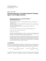
Figure 1: RADARSAT-2 MODEX modes: (a) standard two-
channel receive mode, (b) three-channel half-aperture toggle-
transmit mode, (c) four-channel 3/4-aperture toggle-transmit
mode, and (d) four-channel quarter-aperture toggle-receive mode.
Shaded rectangles constitute active antenna panels with different
shades representing different channels; down/up arrows represent
transmitter/receiver physical center positions, respectively; black
down-pointing triangles denote two-way effective phase centers.
is employed. This would further reduce the achievable SNR.
However, a performance improvement to target parameter
estimation using the sub-aperture switching methodology
has been established theoretically in [32, 33]andwillbe
here demonstrated using recently acquired RADARSAT-2
MODEX data in Section 6.
2. RADARSAT-2 MODEX Modes
The 512 transmit-receive modules (TRMs) in the
RADARSAT-2 two-dimensional active phased array are
organized as 16 columns, as depicted by little rectangles
in Figure 1, with 32 TRMs per column. All TRMs have
independent control of transmitter phase and receiver phase
and amplitude for both vertical and horizontal polarizations
[34]. The phase and amplitude controls in the elevation
dimension allow for the formation and steering of all beams.
Transmitter phase control in the azimuth dimension allows
the formation of the wider beams required for the Ultrafine
resolution mode. This is accomplished by the deliberate
defocussing of the beam [35].
The proposed virtual channel modes take advantage of
the flexible programming capabilities of the RADARSAT-2
antenna to generate two, three, or four phase centers,

as illustrated in Figure 1, using a sub-aperture switching
(or toggling) technique originally proposed by Ender [4].
The spatial diversity of the standard dual-receive mode,
Figure 1(a), can be increased by either transmitter toggling
between pulses, Figures 1(b) and 1(c),orsmartreceiver
excitation schemes, Figure 1(d). These are only a few
methods for achieving multichannel capability and are by
no means exhaustive. Due to transmitter/receiver toggling
between pulses, the pulse repetition frequency (PRF) per
virtualchanneliseffectively cut by one half. This may lead
to clutter band aliasing (non-Nyquist sampling), which may
be partially compensated for by doubling the original PRF.
The half-aperture, toggled-transmit (toggled-Tx) ap-
proach (between fore and aft subapertures), shown in
Figure 1(b), has the advantage of maintaining the same
phase-center distance (or the along-track baseline) as the
standard dual-channel case (Figure 1(a)), which is nominally
3.75 m for RADARSAT-2, and is capable of generating three
independent phase centers, shown as down-pointing trian-
gles. The down/up arrows denote the transmitter/receiver
physical phase center positions, respectively. However, the
two-way beamwidth is significantly increased compared to
the standard dual-channel case due to the half-aperture
transmit. This could lead to clutter band aliasing (as
confirmed by recently acquired MODEX data) even at
RADARSAT-2’s maximum PRF of 3800 Hz (or 1900 Hz per
virtual channel). Also, the half-aperture transmit leads to
a decrease in the transmit power and may severely limit
the attainable SNR. The proposed solution to mitigate this
shortcoming is to increase the transmitter aperture size from

half to three-quarter aperture, as depicted in Figure 1(c).
This sub-aperture switching configuration generates four
independent phase centers (or virtual channels) as repre-
sented by down-pointing triangles at four different positions
along the antenna.
The last approach is the toggled-receive (toggled-Rx) or
sub-aperture switching mode where pulses are transmitted
with the full aperture and returns are received using two
alternating quarter subapertures as shown in Figure 1(d).
Both (c) and (d) modes generate four independent phase
centers and produce an effective phase-center distance that
is one-half that of the standard dual-receive case. The (d)
configuration has a slightly narrower two-way azimuth beam
pattern than that of the (c) case.
The actual antenna patterns of the first three MODEX
modes of Figure 1 have been estimated from recently
acquired RADARSAT-2 MODEX data and are shown in
Figure 2. The corresponding correlation plots between
coregistered channels are also shown. The antenna patterns
for the standard dual-receive mode (Figure 2(a)) and the
3/4-aperture toggled-Tx mode (Figure 2(e)) show that the
clutter bands are adequately sampled using a PRF of 1900 Hz
(per channel). The 1/2-aperture toggled-Tx mode, on the
other hand, shows a 3 dB beamwidth of about 1800 Hz,
which is just below the maximum sampling frequency of
1900 Hz (per channel). Often, the maximum PRF is not
4 EURASIP Journal on Advances in Signal Processing
PDS 0018297 20080812
Relative to maximum (dB)
−14

−12
−10
−8
−6
−4
−2
0
Doppler frequency (Hz)
−1000 −500 0 500
1000 1500
Channel: 1
Channel: 2
(a)
PDS 0018297 20080812
Correlation
0
0.1
0.2
0.3
0.4
0.5
0.6
0.7
0.8
0.9
1
Number of samples shifted
−5 −4 −3 −2 −10 1 2 3 4 5
1
→2: 1

(b)
PDS 0005719 20080320
Relative to maximum (dB)
−3
−2.5
−2
−1.5
−1
−0.5
0
Doppler frequency (Hz)
−500 0 500 1000
1500 2000
Channel: 1
Channel: 2
Channel: 3
Channel: 4
(c)
PDS 0005719 20080320
Correlation
0
0.1
0.2
0.3
0.4
0.5
0.6
0.7
0.8
0.9

1
Number of samples shifted
−50 5
1
→2: 0.9
1
→3: 0.3
1
→4: 1.2
2
→3: −0.5
2
→4: 0.3
3
→4: 1
(d)
PDS 0049383 20090424
Relative to maximum (dB)
−8
−7
−6
−5
−4
−3
−2
−1
0
Doppler frequency (Hz)
−1500 −1000 −500 0 500 1000
Channel: 1

Channel: 2
Channel: 3
Channel: 4
(e)
PDS 0049383 20090424
Correlation
0
0.1
0.2
0.3
0.4
0.5
0.6
0.7
0.8
0.9
1
Number of samples shifted
−5 −4 −3 −2 −10 1 23 4 5
1
→2: 0.9
1
→3: 0
1
→4: 0.9
2
→3: −1
2
→4: 0
3

→4: 0.9
(f)
Figure 2: Estimated antenna patterns and channel correlations for three MODEX modes. (a) and (b) Standard dual-receive mode, (c) and
(d) half-aperture toggle-transmit mode, and (e) and (f) 3/4-aperture toggle-transmit mode.
EURASIP Journal on Advances in Signal Processing 5
Normalised antenna gain
0
0.1
0.2
0.3
0.4
0.5
0.6
0.7
0.8
0.9
1
Frequency (Hz)
−2000 −1500 −1000 −500 0 500 1000 1500 2000
−PRF/2 +PRF/2
Phase ramp multiply
A constant negative phase
offset applied to positive
doppler ambiguities
A constant positive phase
offset applied to negative
doppler ambiguities
Figure 3: Illustrating the interpolation (or time shift) of an
ambiguous clutter signal via the application of a frequency phase
ramp.

achievable due to the duty cycle limitation of RADARSAT-
2. More realistic maximum PRF values often fall in the
range of 3600–3700 Hz (or 1800–1850 Hz per channel).
Therefore, clutter ambiguities can become quite severe for
the 1/2-aperture toggled-Tx mode. It is important to note
that ambiguities must be avoided or minimized, because
they cause decorrelation between coregistered channels due
to interpolation errors [36, 37]asseeninFigure 2(d)
and often generate false moving targets as a result of the
erroneous phase imparted on the ambiguous clutter. These
interpolation errors are illustrated in Figure 3.Tocoregister
channels, the spatially displaced channel signals are time-
shifted, via interpolation, to align them in space. This time
shift is accomplished by applying a phase ramp on the signals
in the frequency domain as illustrated by a solid peach line
in the figure. As the ambiguities fold back into the Doppler
band, the phase ramp is incorrectly applied and imparts a
positive or negative constant phase error (or bias) on these
ambiguous clutter signals, depending on the sign of their
original frequencies. Therefore, ambiguous clutter shows up
as false moving targets in an interferometric SAR image. The
constant phase errors imparted on the ambiguities can be
derived from the Fourier transformation pair: s(t
− τ) ↔
S( f )exp(−j2πτ f), where 2πτ is the slope of the phase ramp
applied to signal S( f ) in the frequency domain to effect the
desired time shift τ on s(t) in the time domain. Therefore,
the constant phase error can be shown to be
δ
φ

=±2πτ f
p
=±
2πτ
T
p
,
(1)
where
± corresponds to ∓ sign in the original frequency of
ambiguous signals, assuming a positive ramp slope, and f
p
and T
p
are the pulse repetition frequency (PRF) and pulse
repetition interval (PRI), respectively. Signs are reversed in
case of a negative ramp. Moreover, one observes from (1)
that the interpolation does not lead to channel decorrelation
if the PRF is chosen to be f
p
= 1/τ, such that the so-called
Displaced Phase Center Antenna (DPCA) condition is met.
Under this condition, there is no sub-sample interpolation
(only integer sample shifting) and the phase errors imparted
on the ambiguities are exactly multiples of 2π, which have
no effect on the signal (including both main and side
beams). The channel-to-channel decorrelation can also be
caused by beam pointing errors, as the beam footprints
for different channels do not coincide perfectly, generating
slightly different clutter Doppler centroid for each channel.

This effect is clearly seen in Figure 2(c), where the Doppler
centroids of different channels differ by up to a few hundreds
of Hertz. The decorrelation caused by the beam pointing
errors is most noticeable for the toggled modes, as seen
in Figure 2(d), where a drop in the correlation is observed
for the interpulse channels. Fortunately, the beam pointing
errors can be easily compensated for by applying a corrective
phase ramp across the elements of a phased array, as was
done for the last case shown in Figure 2(e), where the
errors are reduced down to less than a few tens of Hertz.
With this corrective measure, there is now virtually no drop
in the correlation between the interpulse channels and all
the channels have now correlations over 0.96, as shown in
Figure 2(f).
3. Equations of Motion of a Moving Target
High resolution Synthetic Aperture Radar (SAR) processing
requires that a highly accurate imaging geometry model
be first established. For SAR Ground Moving Target Indi-
cation (SAR-GMTI), the underlying assumption that the
radar scene is stationary must be extended to include
nonstationary scenes or moving targets. This can be quite
easily accomplished for the case of an airborne platform
[38], which is assumed to be moving along a straight line
and transmitting uniformly spaced pulses. This assumption
requires good platform motion compensation and good
control of the PRF as a function of ground speed. The
same cannot be said about a spaceborne platform, where
the earth’s gravitational force plays a key role in defining
the platform trajectory and the velocity of the radar antenna
footprint as it sweeps along the surface of the earth. The

modeling of a moving target for a single channel spaceborne
SAR geometry has already been accomplished to a high
degree of accuracy by Eldhuset [39] and Curlander and
McDonough [40]. However, the extension of the model
to include a SAR system that is equipped with multiple
apertures is evidently absent in the open literature, partly
because there were no existing spaceborne SAR systems
in the unclassified world equipped with such a capability
up until the recent launches of COSMO-SkyMed [11],
TerraSAR-X [41] and RADARSAT-2 [13] in 2007. In the
following, equations of motion of a ground moving target
for a multichannel spaceborne SAR are derived. The full
derivation is presented here for the first time, although this
model has been used in our previous work.
Several assumptions are used to simplify the model. The
SAR pointing angles, measured from a reference pointing
direction, are assumed to be small. The along-track speed
of the target is assumed to be much smaller than the SAR
platform speed, which is warranted in the case of spaceborne
SAR and typical ground vehicles. It is also assumed that the
rate of change is very slow for certain orbital parameters,
6 EURASIP Journal on Advances in Signal Processing
such as the linear speed, which is true for nearly circular
orbits. For the sake of generality, these assumptions are not
incorporated in the statement of the problem. They are
introduced, where appropriate, only to simplify the final
formulae. For a different SAR system, they may be reviewed
or removed at the expense of model complexity.
The relative position vector of a moving target with
respect to an imaging SAR satellite, in the earth centered

earth fixed (ECEF) system, can be written as
R
= R
t
− R
s
,
(2)
where indices “t” and “s” denote “target” and “satellite,”
respectively. A bold letter indicates a vector and the
corresponding regular italic font (of the same symbol)
represents the magnitude of the vector, and a bold upper
case letter represents a matrix. In the ECEF frame, the earth
motion is absorbed into the relative satellite motion.
The Doppler centroid and Doppler rate are proportional
to
˙
R and
¨
R, respectively, where the dot and double-dot
notations indicate first and second derivatives with respect
to time. A common approach to the derivation of
˙
R and
¨
R is
to start from the identity [40]
R
2
= R

T
R
(3)
and to differentiate it with respect to time, where superscript
“T” denotes the vector (or matrix) transpose.
Differentiating both sides of (3)withrespecttotime,we
get
2R
˙
R
=
˙
R
T
R + R
T
˙
R
,(4a)
˙
R
=
R
T
˙
R
R
.
(4b)
Equation (4b)canberewrittenas

˙
R
=
R
T
R
(
V
t
− V
s
)
(5a)
= V
tr
− V
sr
,(5b)
where V
t
≡
˙
R
t
is the velocity vector of the moving target,
V
s
≡
˙
R

s
is the velocity vector of the satellite, and
V
tr
≡

R
R

T
V
t
,
V
sr
≡

R
R

T
V
s
,
(6)
are the projections of the target and satellite velocity vectors,
respectively, onto the line of sight (LOS) or the radial
direction. Also, the radial speed of a stationary target as
“seen” by the radar due to the platform motion is equal
to

−V
sr
. Therefore, the Doppler shift at the beam center
induced by the motion of the platform (or the stationary
clutter Doppler centroid) is given by
f
DC
= 2
V
sr
λ
,(7)
and the Doppler shift due to the target’s radial speed is
f
dc
=−2
V
tr
λ
. (8)
Therefore, the total Doppler shift is given by
F
DC
=−2
V
r
λ
=−2
(
V

tr
− V
sr
)
λ
.
(9)
Again, differentiating both sides of (4a)withrespectto
time yields
2

˙
R
2
+ R
¨
R

=
2R
T
¨
R
+2
˙
R
T
˙
R
, (10a)

R
¨
R
= R
T
¨
R
+
˙
R
T
˙
R
−
˙
R
2
.
(10b)
Using the following definitions
V
t
≡
˙
R
t
,
V
s
≡

˙
R
s
,
A
t
≡
¨
R
t
,
A
s
≡
¨
R
s
,
A
≡
¨
R
=
¨
R
t
−
¨
R
s

= A
t
− A
s
,
A
tr
≡
R
T
A
t
R
,
(11)
Equation (10b)canberewrittenas
R
¨
R
= R

R
T
R
A
t

−
R
T

A
s
+
(
V
t
−V
s
)
T
(
V
t
−V
s
)
−
(
V
tr
−V
sr
)
2
= RA
tr
− R
T
A
s

+ V
2
t
− V
T
t
V
s
− V
T
s
V
t
+ V
2
s
−

V
2
tr
− 2V
tr
V
sr
+ V
2
sr

=

V
2
s
− R
T
A
s
+ RA
tr
+ V
2
t
− 2V
s

V
T
s
V
s
V
t

−
V
2
tr
+2V
tr
V

sr
− V
2
sr
.
(12)
Therefore,
¨
R
=
V
2
e
R
−
V
2
sr
R
+ A
tr
+
V
2
t
R
−
2V
s
V

ta
R
−
V
2
tr
R
+
2V
tr
V
sr
R
,
(13)
where
V
2
e
≡ V
2
s
− R
T
A
s
, (14a)
V
ta
=


V
s
V
s

T
V
t
.
(14b)
V
e
is the so-called “effective velocity” often used in the
spaceborne SAR processing to model the range equation and
V
ta
is the projection of the target velocity onto the direction
of platform velocity V
s
(also called the along-track direction)
and needs not to be parallel to the ground track.
EURASIP Journal on Advances in Signal Processing 7
The instantaneous slant range equation (or history) R(t)
is the key to high precision SAR processing. Accurate esti-
mation of the effective velocity V
e
allows complicated math-
ematical manipulations involving a satellite/earth geometry
model to be avoided and a simple hyperbolic approximation

to be adopted in most high precision SAR processing
algorithms [42]. The hyperbolic model can be further
simplified and approximated using a second-order Taylor
series expansion or a parabolic model without significantly
incurring further loss of accuracy for typical RADARSAT-2
dwell times and resolutions. However, this may not be true
in general.
If
˙
R and
¨
R in (5a)and(13)areevaluatedatsomearbi-
trary time t
0
, then the range equation can be approximated
by the Taylor series expansion:
R
(
t
)
≈ R
0
+ V
r0
(
t
− t
0
)
+

A
r0
2
(
t
− t
0
)
2
,
(15)
where
R
0
= R
(
t
0
)
=|R
t
(
t
0
)
− R
s
(
t
0

)
| (16a)
V
r0
=
˙
R
(
t
0
)
=
R
T
0
R
0
[
V
t
(
t
0
)
− V
s
(
t
0
)

]
= V
tr
− V
sr
(16b)
A
r0
=
¨
R
(
t
0
)
=
V
2
e
− V
2
sr
R
0
+
V
2
t
− V
2

tr
+2V
tr
V
sr
− 2V
s
V
ta
R
0
+ A
tr
(16c)
≈
V
2
e
− V
2
sr
R
0
+
2V
tr
V
sr
− 2V
s

V
ta
R
0
+ A
tr
. (16d)
V
2
t
and V
2
tr
are considered negligible with respect to 2V
s
V
ta
and, therefore, are dropped in (16d). If t
0
is chosen to be
the broadside time t
b
, then V
sr
= 0 by definition and
the radial direction (subscripted by “r”) becomes exactly
perpendicular to the flight direction or the along-track
direction (subscripted by “a”). Under this condition, (16b)
and (16d)become
V

rb
=
˙
R
(
t
b
)
=
R
T
b
R
b
V
t
(
t
b
)
= V
tr
,
(17a)
A
rb
=
¨
R
(

t
b
)
≈
V
2
e
− 2V
s
V
ta
R
b
+ A
tr
,
(17b)
where V
tr
and A
tr
are now the target’s down-range (or across-
track) velocity and acceleration components, respectively,
and R
b
is the broadside range of the moving target. In the
vicinity of t
b
, therefore, the Taylor series expansion reads
R

(
t
)
≈ R
b
+ V
tr
(
t
− t
b
)
+
A
rb
2
(
t
− t
b
)
2
.
(18)
The use of a parabolic model is convenient in the
derivation of range equations for multichannel SAR systems.
In the following, the range equation for the second aperture
of a two-channel SAR is derived.
V
s

f
r
u
u
0
d
θ
sin θ
cos θ
+ϕ
p
+ϕ
y
Figure 4: Local reference frame of radar.
3.1. Local Frame of Reference. In order to continue with
our derivations, we first define a local flight (LF) frame of
reference for the radar as shown in Figure 4,whered is
defined as the unit vector pointing down from the radar’s
center of gravity to the center of the earth. To define the
second axis, we cross (vector) multiply d with the radar’s
velocity vector V
s
to form the right pointing unit vector r:
r
=
d × V
s
|d × V
s
|

.
(19)
Then the third unit vector, which completes the local
reference frame, is given by
f
= r × d.
(20)
We should point out that V
s
is not necessarily in the exact
same direction as f,asillustratedinFigure 4.
3.2. Transformation Matrix. We now derive the transfor-
mation matrix from the LF reference frame to the ECEF
reference frame. To begin, we express the unit vector d in the
ECEF frame:
d
=−
R
s
|R
s
|
=−
1
R
s
⎡
⎢
⎢
⎢

⎣
R
sx
R
sy
R
sz
⎤
⎥
⎥
⎥
⎦
(21)
Then r becomes
r
=
d × V
s
|d × V
s
|
=
1
R
s
V
hor
⎡
⎢
⎢

⎢
⎣
R
sz
V
sy
− R
sy
V
sz
R
sx
V
sz
− R
sz
V
sx
R
sy
V
sx
− R
sx
V
sy
⎤
⎥
⎥
⎥

⎦
,
(22)
8 EURASIP Journal on Advances in Signal Processing
where
V
hor
=|d × V
s
|,
V
s
=
⎡
⎢
⎢
⎢
⎣
V
sx
V
sy
V
sz
⎤
⎥
⎥
⎥
⎦
.

(23)
V
hor
is obviously the horizontal velocity component of the
radar and can be easily shown to be
V
hor
=

V
2
sx
+ V
2
sy
+ V
2
sz
− V
2
ver
,
(24)
where V
ver
is the vertical velocity component of the radar
platform and is given by
V
ver
=

R
T
s
R
s
V
s
=
R
sx
V
sx
+ R
sy
V
sy
+ R
sz
V
sz
R
s
.
(25)
We are now ready to express the forward unit vector f in the
ECEF frame as
f
= r × d =−d × r
=
1

R
s
V
hor
⎡
⎢
⎢
⎢
⎣
R
s
V
sx
− R
sx
V
ver
R
s
V
sy
− R
sy
V
ver
R
s
V
sz
− R

sz
V
ver
⎤
⎥
⎥
⎥
⎦
.
(26)
Finally, the transformation matrix from the LF reference
frame to the ECEF frame [43] is simply
Γ
f
=

frd

(27a)
=
1
R
s
V
hor
⎡
⎢
⎢
⎢
⎣

R
s
V
sx
− R
sx
V
ver
R
sz
V
sy
− R
sy
V
sz
−R
sx
V
hor
R
s
V
sy
− R
sy
V
ver
R
sx

V
sz
− R
sz
V
sx
−R
sy
V
hor
R
s
V
sz
− R
sz
V
ver
R
sy
V
sx
− R
sx
V
sy
−R
sz
V
hor

⎤
⎥
⎥
⎥
⎦
.
(27b)
3.3. Antenna Look Vector. Let the ideal look direction of the
antenna in the LF frame, with an off-nadir angle θ pointing
at a zero Doppler point on the surface of the earth, be
u
0
=
⎡
⎢
⎢
⎢
⎣
0
sin θ
cos θ
⎤
⎥
⎥
⎥
⎦
. (28)
Then the actual antenna look vector (or pointing vector) in
the local reference frame of the radar is given by
u = Γ

ϕ
u
0
(29a)
≈
⎡
⎢
⎢
⎢
⎣
−
ϕ
y
sin θ + ϕ
p
cos θ
sin θ
cos θ
⎤
⎥
⎥
⎥
⎦
, (29b)
where Γ
ϕ
is the yaw-pitch rotation matrix, and ϕ
y
and ϕ
p

are
the yaw and pitch angles about the axes d and r,respectively.
We are assuming that ϕ
y
and ϕ
p
correspond to a LOS within
the beam, but not necessarily at its center. For RADARSAT-
2, ϕ
y
and ϕ
p
are typically small (1) in the ECEF frame due
to the mechanical zero-Doppler beam steering. The rotation
matrix Γ
ϕ
can, therefore, be shown to be
Γ
ϕ
= M
r
M
d
(30a)
≈
⎡
⎢
⎢
⎢
⎣

1 −ϕ
y
ϕ
p
ϕ
y
10
−ϕ
p
01
⎤
⎥
⎥
⎥
⎦
, (30b)
where
M
r
=
⎡
⎢
⎢
⎢
⎣
cos ϕ
p
0sinϕ
p
010

−sin ϕ
p
0cosϕ
p
⎤
⎥
⎥
⎥
⎦
≈
⎡
⎢
⎢
⎢
⎣
10ϕ
p
010
−ϕ
p
01
⎤
⎥
⎥
⎥
⎦
,
M
d
=

⎡
⎢
⎢
⎢
⎣
cos ϕ
y
−sin ϕ
y
0
sin ϕ
y
cos ϕ
y
0
001
⎤
⎥
⎥
⎥
⎦
≈
⎡
⎢
⎢
⎢
⎣
1 −ϕ
y
0

ϕ
y
10
001
⎤
⎥
⎥
⎥
⎦
.
(31)
The term, ϕ
y
ϕ
p
, is considered negligible [43] and is set to
zero in (29b)and(30b). In the ECEF frame, the antenna look
vector u is then given by
u
= Γ
f
u = Γ
f
Γ
ϕ
u
0
.
(32)
Note that the look vector u is not necessarily in the direction

of the beam center, rather it points to the direction of the
target of interest within the beam footprint.
3.4. Displacement Vector. Let

D denote the vector pointing
from the effective phase center of the aft sub-aperture to
the effective phase center of the fore sub-aperture in the LF
frame, then

D can be expressed as

D = Γ
ψ
⎡
⎢
⎢
⎢
⎣
D
0
0
⎤
⎥
⎥
⎥
⎦
≈
D
⎡
⎢

⎢
⎢
⎣
1
ψ
y
−ψ
p
⎤
⎥
⎥
⎥
⎦
, (33)
where
Γ
ψ
= Γ
ϕ

ϕ = ψ

≈
⎡
⎢
⎢
⎢
⎣
1 −ψ
y

ψ
p
ψ
y
10
−ψ
p
01
⎤
⎥
⎥
⎥
⎦
, (34)
and ψ
y
and ψ
p
are the pitch and yaw angles (or the
orientation) of the antenna, representing the attitude of the
spacecraft in the LF frame of reference. In the ECEF frame,

D
becomes
D
= Γ
f

D = DΓ
f

⎡
⎢
⎢
⎢
⎣
1
ψ
y
−ψ
p
⎤
⎥
⎥
⎥
⎦
. (35)
EURASIP Journal on Advances in Signal Processing 9
3.5. Range Equations for Multiple Phase Centers. Atwo-
aperture SAR-GMTI system is again assumed in the fol-
lowing derivations with the understanding that the derived
equations can be generalized to a multiaperture system. Let
R
s1
and R
s2
denote the position vectors of the antenna’s
two effective (or two-way) phase centers in the ECEF
frame, respectively. The aft antenna phase center R
s2
is then

displaced from the fore antenna phase center R
s1
by −D.
For the case of RADARSAT-2, the displacement vector D is
closely aligned with the radar’s velocity vector V
s
.Perfect
alignment would be optimal because it would allow the
aft phase center to pass through the same ECEF position
as the fore phase center with a time delay of τ
= D/V
s
,
where D is the distance between the two effective phase
centers. This perfect alignment would also mean that the
whole antenna is ideally steered, generating a zero Doppler
centroid in the clutter Doppler spectrum. In the presence of
a nonzero Doppler centroid, there exists a nonzero across-
track component of D, which translates into a small across-
track baseline. In the case of a real spaceborne SAR-GMTI
system, such as the RADARSAT-2 MODEX, this small cross-
track component is always present and, therefore, must
be compensated for or taken into account in the system
modeling [19].
The slant-range vector R
2
from the aft antenna phase
center to the target can, therefore, be expressed as
R
2

= R
t
− R
s2
(36a)
= R
1
+ D, (36b)
where R
1
= R
t
−R
s1
and R
s2
= R
s1
−D. Then the projections
of these slant-range vectors, R
1
and R
2
, along the look vector
u direction are given by
R
1
= R
T
1

u, (37a)
R
2
= R
T
2
u =

R
T
1
+ D
T

u = R
1
+ D
T
u (37b)
= R
1
+

Γ
f

D

T
Γ

f
u = R
1
+

D
T
Γ
T
f
Γ
f
u (37c)
= R
1
+

D
T
u. (37d)
From (29b)and(33), (37d)becomes
R
2
(
t
)
≈ R
1
(
t

)
+ D

1 ψ
y
−ψ
p

⎡
⎢
⎢
⎢
⎣
−
ϕ
y
sin θ + ϕ
p
cos θ
sin θ
cos θ
⎤
⎥
⎥
⎥
⎦
(38a)
= R
1
(

t
)
+ D

ψ
y
− ϕ
y

sin θ −

ψ
p
− ϕ
p

cos θ

(38b)
= R
1
(
t
)
+ D
(
Ψ
− Φ
)
, (38c)

where
Ψ
= ψ
y
sin θ − ψ
p
cos θ,
Φ
= ϕ
y
sin θ − ϕ
p
cos θ.
(39)
Ψ and Φ are now measured in the slant-range plane. As
the antenna footprint sweeps across the target, the pitch
angle ϕ
p
hardly changes (i.e., remains virtually constant)
such that ϕ
p
≈ ψ
p
, resulting in Ψ − Φ ≈ (ψ
y
− ϕ
y
)sinθ.
In the case of RADARSAT-2, ψ
y

and ψ
p
are usually small
but nonzero such that the beam center is not located exactly
at the zero-Doppler point on the surface of the earth (in
the ECEF frame). This residual beam squint Ψ generates
a small constant along-track interferometric phase, which
is usually removed by the digital-balance processing of the
signal channels and can, therefore, be ignored. For the sake
of completeness, however, we shall keep the term in (38c).
Then, the zeroth-order coefficient of the Taylor expansion of
R
2
(t) evaluated at arbitrary time t
0
can be expressed as
R
2
(
t
0
)
= R
1
(
t
0
)
− D
[

Φ
(
t
0
)
− Ψ
]
.
(40)
Next, we derive the first-order coefficient of the Taylor
series expansion of R
2
(t). From (36b), we obtain
R
2
2
=
(
R
1
+ D
)
T
(
R
1
+ D
)
, (41a)
R

2
˙
R
2
=
(
R
1
+ D
)
T

˙
R
1
+
˙
D

, (41b)
˙
R
2
=
R
T
1
˙
R
1

+ R
T
1
˙
D + D
T
˙
R
1
+ D
T
˙
D
R
2
(41c)
=
R
1
˙
R
1
R
2
+
R
T
1
˙
D

R
2
+
D
T
˙
R
1
R
2
+
D
T
˙
Γ
f

D
R
2
(41d)
≈
˙
R
1
+
R
T
R
˙

D +
D
T
R
˙
R +
O

D
2

R
(41e)
≈
˙
R
1
+ u
T
˙
D +
D
T
R
(
V
t
− V
s
)

, (41f)
where it can be shown that R
T
1
˙
R
1
= R
1
˙
R
1
, R
1
≈ R
2
= R,and
the O(D
2
) term can be neglected.
First, we derive the second term in (41f):
u
T
˙
D
= u
T
∂
∂t


Γ
f

D

=
u
T

˙
Γ
f

D + Γ
f
˙

D

=
u
T
˙
Γ
f

D,
(42)
where we have assumed that the spacecraft attitude is not
changing in the LF frame such that time derivatives of ψ

y
and ψ
p
(or
˙

D) are equal to zero in the imaging time interval.
We also assume, for simplicity, that ψ
y
and ψ
p
are small
(normally true for RADARSAT-2). Therefore, (42)becomes
u
T
˙
D
= u
T
˙
Γ
f
D
⎡
⎢
⎢
⎢
⎣
1
ψ

y
−ψ
p
⎤
⎥
⎥
⎥
⎦
≈
u
T
˙
Γ
f
D
⎡
⎢
⎢
⎢
⎣
1
0
0
⎤
⎥
⎥
⎥
⎦
. (43)
Here, we need to find the first time derivative of Γ

f
(i.e.,
˙
Γ
f
),
which can be shown to be
10 EURASIP Journal on Advances in Signal Processing
˙
Γ
f
=
1
R
s
V
hor
⎡
⎢
⎢
⎢
⎣
˙
R
s
V
sx
+ R
s
A

sx
− V
sx
V
ver
− R
sx
˙
V
ver
R
sz
A
sy
− R
sy
A
sz
−V
sx
V
hor
− R
sx
˙
V
hor
˙
R
s

V
sy
+ R
s
A
sy
− V
sy
V
ver
− R
sy
˙
V
ver
R
sx
A
sz
− R
sz
A
sx
−V
sy
V
hor
− R
sy
˙

V
hor
˙
R
s
V
sz
+ R
s
A
sz
− V
sz
V
ver
− R
sz
˙
V
ver
R
sy
A
sx
− R
sx
A
sy
−V
sz

V
hor
− R
sz
˙
V
hor
⎤
⎥
⎥
⎥
⎦
, (44)
where terms of the type V
sx
V
sy
, V
sx
V
sz
,andV
sz
V
sy
cancel out
in the second column of (44) and are, therefore, dropped. We
can further simplify (44) by noting that
˙
R

s
≈ 0,
˙
V
hor
≈ 0, and
˙
V
ver
≈ 0:
˙
Γ
f
≈
1
R
s
V
hor
⎡
⎢
⎢
⎢
⎣
R
s
A
sx
− V
sx

V
ver
R
sz
A
sy
− R
sy
A
sz
−V
sx
V
hor
R
s
A
sy
− V
sy
V
ver
R
sx
A
sz
− R
sz
A
sx

−V
sy
V
hor
R
s
A
sz
− V
sz
V
ver
R
sy
A
sx
− R
sx
A
sy
−V
sz
V
hor
⎤
⎥
⎥
⎥
⎦
.

(45)
Therefore, (43)becomes
u
T
˙
D
≈
D
R
s
V
hor
u
T
⎡
⎢
⎢
⎢
⎣
R
s
A
sx
− V
sx
V
ver
R
s
A

sy
− V
sy
V
ver
R
s
A
sz
− V
sz
V
ver
⎤
⎥
⎥
⎥
⎦
(46a)
=
D
V
hor
u
T
A
s
−
DV
ver

R
s
V
hor
u
T
V
s
(46b)
≈
D
V
hor
u
T
A
s
. (46c)
The last term in (46b) is ignored since the look vector u is
virtually perpendicular to V
s
.
We now derive the last term of (41f). From (27b)and
(35),
D
T
R
(
V
t

− V
s
)
=
D
R

1 ψ
y
−ψ
p

Γ
T
f
(
V
t
− V
s
)
(47a)
≈
D

R
s
V
sx
− R

sx
V
ver
R
s
V
sy
− R
sy
V
ver
R
s
V
sz
− R
sz
V
ver

RR
s
V
hor
×
⎛
⎜
⎜
⎜
⎝

V
t
−
⎡
⎢
⎢
⎢
⎣
V
sx
V
sy
V
sz
⎤
⎥
⎥
⎥
⎦
⎞
⎟
⎟
⎟
⎠
,
(47b)
where ψ
y
 1, ψ
p

 1, and they are neglected in (47b). Also
by noting that
R
s
V
T
s
− V
ver
R
T
s
=

R
s
V
sx
− R
sx
V
ver
R
s
V
sy
− R
sy
V
ver

R
s
V
sz
− R
sz
V
ver

,
R
s
= R
s
+ R
t
− R
t
= R + R
t
,
V
T
s
V
t
= V
s
V
ta

,
(
R + R
t
)
T
V
t
= RV
tr
+ R
T
t
V
t
≈ RV
tr
,
(48)
where V
t
is virtually perpendicular to R
t
for ground moving
targets, we can rewrite (47b)as
D
T
R
(
V

t
− V
s
)
≈
D
RR
s
V
hor

R
s
V
T
s
− V
ver
R
T
s

V
t

+
D
RR
s
V

hor
×

−R
s
V
2
s
+ V
ver

R
sx
V
sx
+ R
sy
V
sy
+ R
sz
V
sz

(49a)
= D

V
s
V

hor

V
ta
R
−

V
ver
V
hor

V
tr
R
s
−

V
s
V
hor

V
s
R
+

V
ver

V
hor

V
ver
R

.
(49b)
Finally, (49b) can be further simplified by noting that V
hor
≈
V
s
and V
ver
/V
hor
 1, yielding
D
T
R
(
V
t
− V
s
)
≈
D

R
(
V
ta
− V
s
)
.
(50)
Putting everything together, (41f)becomes
˙
R
2
=
˙
R
1
+
D
V
hor
u
T
A
s
+
D
R
(
V

ta
− V
s
)
(51a)
≈
˙
R
1
+
D
R
V
ta
−
D
RV
s

V
2
s
− R
T
A
s

=
˙
R

1
−
D
R

V
2
e
V
s
− V
ta

(51b)
≈
˙
R
1
−
D
R

V
g
− V
ta

, (51c)
where we make use of V
2

e
≡ V
2
s
− R
T
A
s
(14a)andV
g
≈
V
2
e
/V
s
. The latter is the velocity of the beam footprint that
EURASIP Journal on Advances in Signal Processing 11
moves along the surface of the earth and the approximation
is mainly due to the fact that the satellite orbit is only
approximately circular. Therefore, the first-order coefficient
of the Taylor expansion of R
2
(t) evaluated at time t
0
can be
written as
˙
R
2

(
t
0
)
=
˙
R
1
(
t
0
)
−
D
R
(
t
0
)

V
g
− V
ta

=
(
V
tr
− V

sr
)
−
D
R
(
t
0
)

V
g
− V
ta

.
(52)
Similarly, we derive the second-order coefficient of the
Taylor series expansion of R
2
(t) by taking the time derivative
of (51c), which simply yields
¨
R
2
≈
¨
R
1
. Therefore, the Taylor

expansion of R
2
(t) (up to the second order) evaluated at
arbitrary time t
0
can be written as
R
2
(
t
)
= R
(
t
0
)
− D
[
Φ
(
t
0
)
− Ψ
]
+

(
V
tr

− V
sr
)
−
D
R
(
t
0
)

V
g
− V
ta


(
t
− t
0
)
+
1
2

V
2
e
− 2V

s
V
ta
R
(
t
0
)
+ A
tr

(
t
− t
0
)
2
.
(53)
We are now ready to generalize the moving target range
equation (53) for a multichannel SAR system (i.e., with
multiple phase centers)
R
p
(
t
)
= R
0
+


p −1

D
(
Ψ − Φ
0
)
+
(
V
tr
− V
sr
)(
t
− t
0
)
+

p −1

D
R
0

V
ta
− V

g

(
t
− t
0
)
+
1
2

V
2
e
− 2V
s
V
ta
R
0
+ A
tr

(
t
− t
0
)
2
,

(54)
where R
0
= R(t
0
), Φ
0
= Φ(t
0
); V
tr
, V
ta
,andA
tr
are defined
for time t
0
; p = 1, 2, 3, (for equidistant phase center 1,
2, 3, etc.); V
sr
depends on V
s
and Φ
0
in a predictable way;
V
s
, V
g

,andV
e
vary slowly with time and, therefore, may be
evaluated anywhere in the neighborhood of t
0
.
If we choose t
0
to be the broadside time t
b
, then Φ and
V
sr
(=−V
s
Φ) become zero, resulting in
R
p
(
t
)
= R
b
+

p −1

DΨ + V
tr
(

t
− t
b
)
+

p −1

D
R
b

V
ta
− V
g

(
t
− t
b
)
+
1
2

V
2
e
− 2V

s
V
ta
R
b
+ A
tr

(
t
− t
b
)
2
,
(55)
where subscript “b” denotes the broadside time. In order
to generate an interferogram or a SAR-DPCA image, one
normally performs coregistration of channels with respect to
channel 1 (p
= 1). Therefore, the range history (55)ofa
coregistered channel p becomes
R
p

t +

p −1

D

V
s

≈
R
1
(
t
)
+

p −1

D

Ψ +
V
tr
V
s
+

A
tr
V
s
−
V
ta
R

b

(
t
− t
b
)

,
(56)
where terms containing D
2
/V
2
s
or D
2
/(V
s
R
b
)havebeen
neglected in the equation.
When examining a target track acquired by a real-world
SAR, one observes that it has breaks and missing portions
[38], during which times the target fades out and appears
invisible to the radar. As a result, the effective center of the
track may not always correspond to the boresight (or the
beam-center) time of the target. If the actual measured target
track (or range history) is centered at t

= t
b
+ δ for δ =
δ
Ψ
+ δ
c
,whereδ
Ψ
and δ
c
are the time offsets due to the beam
squint and the target track not being effectively centered at
the beam boresight, respectively, then the coregistered signals
for channels 1 and p can be written, respectively, as
s
1
= rect

t −t
b
− δ
T

exp

−
j
4π
λ

R
1
(
t
)

,
(57a)
s
p
= rect

t −t
b
− δ
T

exp

−
j
4π
λ
R
p

t +

p −1


D
V
s

,
(57b)
where j
=
√
−1, T ( D/2V
s
) is the length of the signal,
and, for simplicity, rect[
·] is the idealized two-way antenna
pattern.
The accuracy of the equations of motion derived above
is validated and demonstrated in Section 6 by applying the
parameter estimation algorithm, described in Section 4,to
the recently acquired RADARSAT-2 MODEX data.
4. Parameter Estimation Algorithm
We describe here a target parameter estimation algorithm
based on the fractional Fourier transform (FrFT) [44]and
along-track interferometry (ATI) [45], also called the Frac-
trum Estimator, for the RADARSAT-2 imaging geometry.
Equations that relate various target parameters are derived.
The FrFT, with fractional frequency variable u and
rotational angle α,ofasignal f (t)isdefinedas[44]
F
α
(

u
)
= R
α

f

(
u
)
=

∞
−∞
f
(
t
)
K
α
(
t, u
)
dt,
(58)
where, for α being not equal to zero or a multiple of π, the
kernel K
α
(t, u)isgivenby
K

α
(
t, u
)
= c exp

j2πa

t
2
+ u
2
− 2but

,
a
=
cot α
2
, b
= sec α, c =

1 − jcotα.
(59)
TheFrFTwithparameterα canbeconsideredasagener-
alization of the conventional Fourier transform (FT). Thus,
12 EURASIP Journal on Advances in Signal Processing
the FrFT for α
= π/2andα =−π/2 reduces to the
conventional and inverse FT, respectively.

The FrFT is first applied to each detected target to focus
its signals (received at different channels or subapertures) in
the fractional Fourier domain. The best focus is achieved by
searching for a fractional parameter α that maximizes the
DPCA output of the target. Combining (18)and(57a) into
(58) and integrating to maximize the target signal in the
fractional Fourier domain yield
F
α1
(
u
)
= exp

j
1


+∞
−∞
rect

t −t
b
− δ
T

exp

j


ξ
1
t + ν
1
t
2

dt
(60)
= exp

j
1


t
b
+δ+T/2
t
b
+δ−T/2
exp

jξ
1
t

dt (61)
= exp


j
[

1
+ ξ
1
(
t
b
+ δ
)
]

2
ξ
1
×
exp

jξ
1
T/2

− exp

−jξ
1
T/2


2j
(62)
= exp

j
[

1
+ ξ
1
(
t
b
+ δ
)
]

Tsinc

ξ
1
T
2π

, (63)
where one gathers the terms for t
0
, t
1
,andt

2
,respectively,to
yield

1
= 2πau
2
+2k

V
tr
t
b
−
A
rb
2
t
2
b
− R
b

,
(64a)
ξ
1
=−4π

f

p
√
N

abu −2k
(
V
tr
− A
rb
t
b
)
, (64b)
ν
1
= 2π

f
2
p
N

a − kA
rb
= 0,
(64c)
where k
= 2π/λ is the wavenumber, N is the number
of processed pulses, and time scaling f

p
/
√
N has been
applied. The scaling is necessary when passing from physical
quantities to the normalized unitless variables used in the
digital implementation of the FrFT.
The target signal amplitude is maximized in the frac-
tional Fourier domain if ν
1
in (64c)issetequaltozero,which
yields a “sinc” function in (63) and the optimum fractional
angle α:
α
= cot
−1

NkA
rb
f
2
p
π

.
(65)
Similarly, the optimum fractional Fourier transform of the
signal received at channel p can be shown to be
F
αp

(
u
)
= exp

j


p
+ ξ
p
(
t
b
+ δ
)

T sinc

ξ
p
T
2π

, (66)
where

p
= 
1

− 2k

p −1

D

−

V
ta
− V
g
R
b
+
A
rb
V
s

t
b
+
V
tr
V
s
+ Ψ

,

(67a)
ξ
p
= ξ
1
− 2k

p −1

D

V
ta
− V
g
R
b
+
A
rb
V
s

=
ξ
1
− 2k

p −1


D

A
tr
V
s
−
V
ta
R
b

.
(67b)
Therefore, the phase of the interferogram (arg[F
α1
(u)F
αp
(
u
)
∗
])
evaluated at the optimum fractional Fourier angle α yields
ψ
1p
= 
1
+ ξ
1

(
t
b
+ δ
)
−


p
+ ξ
p
(
t
b
+ δ
)

(68a)
= 
1
− 
p
+

ξ
1
− ξ
p

(

t
b
+ δ
)
(68b)
= 2k

p −1

D

V
tr
V
s
+ Ψ

+

V
ta
− V
g
R
b
+
A
rb
V
s


δ

.
(68c)
Equation (68c) seems to indicate that ψ
1p
is sensitive
to both the across-track (or slant-range) speed V
tr
and
the along-track speed V
ta
. This is due to RADARSAT-2’s
antenna squint, which introduces the along-track velocity
dependence of ψ
1p
in the direction of radar-to-target line
of sight. The result differs from that of the nonsquint case,
which depends only on the target’s across-track velocity
component [38]. However, from (17b) the second term
inside the square bracket of (68c) is shown to be

V
ta
− V
g
R
b
+

A
rb
V
s

δ ≈

−
V
ta
R
b
+
A
tr
V
s

δ,
(69)
which is negligible compared to the first term in (68c)
for typical RADARSAT-2 imaging geometries and common
ground vehicles. This important result, which differs from
that of an airborne case [38], essentially decouples the
parameter estimation equations, even for large δ values.
Therefore, the formula for estimating the target range speed
V
tr
simplifies to
V

tr
=
ψ
1p
V
s
2k

p −1

D
,
(70)
where Ψ in (68c) can be estimated from the phase of the
clutter interferogram (for any two coregistered channels)
and is removed during the channel-balance processing and,
therefore, dropped in (70).
The positions of a moving target in the fractional Fourier
axis for channels 1 and p can be derived by setting ξ
1
= 0
(64b)andξ
p
= 0(67b), respectively. That is, evaluating at
the maxima of the “sinc” functions in (63)and(66) yields
u
1
=
k
2πab


√
N
f
p

[
A
rb
t
b
− V
tr
]
, (71a)
u
p
=
k
2πab

√
N
f
p


A
rb
t

b
− V
tr
−

p −1

D

A
tr
V
s
−
V
ta
R
b

.
(71b)
EURASIP Journal on Advances in Signal Processing 13
The third and fourth terms in (71b) can be ignored
compared to the first two terms, and
u
1
−u
p
is smaller than
the spatial resolution of “sinc” functions, implying spatial

overlap on the fractional Fourier axis or u
1
= u
p
= u
t
.
Therefore, the target broadside azimuth position x
b
(=V
g
t
b
)
can be obtained directly from (71a) by solving for t
b
:
t
b
=
1
A
rb

2πabu
t
k

f
p

√
N

+ V
tr

, (72)
where u
t
is the measured target position on the unitless
fractional Fourier axis and A
rb
is obtained from the estimated
α that best focuses the target energy in the fractional Fourier
domain using (65):
A
rb
=

f
2
p
N

π
k
cot α.
(73)
Finally, the target along-track speed is estimated from (17b):
V

ta
=
V
2
e
− R
b
A
rb
2V
s
,
(74)
where a nonaccelerating target is assumed (i.e., A
tr
= 0). If
the target is accelerating with a constant A
tr
, then one must
use other information to decouple V
ta
and A
tr
contained in
A
rb
. This case, however, will not be considered in this paper.
In summary, the equations used for estimating V
ta
, V

tr
,
and t
b
are
V
ta
=
V
2
e
− R
b
A
rb
2V
s
,
V
tr
=
ψ
1p
V
s
2k

p −1

D

,
t
b
=
1
A
rb

2πabu
t
k

f
p
√
N

+ V
tr

,
(75)
where
A
rb
=

f
2
p

N

π
k
cot α,
a
=
cot α
2
,
b
= sec α,
(76)
V
e
= satellite effective speed, calculated from satellite state
vectors, V
s
= satellite velocity in ECEF frame, R
b
= distance
fromradartodetectedtargetwhenitisatradarbroadside,
ψ
1p
= interferometric phase of coregistered channels (1 and
p)focusedviaFrFT,p
= channel number, k = wavenumber,
D
= distance between two effective phase centers, u
t

=
position of focused target on fractional Fourier axis, f
p
=
azimuth sampling or pulse repetition frequency, N = target
signal length or the number of azimuth pulses, α
= fractional
angle or parameter used to best focus the target, V
ta
=target’s
estimated azimuth speed, V
tr
=target’s estimated slant-range
speed, and t
b
= target’s estimated broadside time.
The FrFT-ATI parameter estimation algorithm (or the
Fractrum Estimator) can be summarized as consisting of the
following nine steps
(1) after detection, extract moving target signals from
range-compressed, azimuth-uncompressed raw data
for channels 1 and p;
(2) apply DPCA processing on the signals;
(3) find fractional parameter α that best focuses the
DPCA image of the moving target;
(4) measure target position u
t
on the fractional Fourier
axis;
(5) using the optimum α value, calculate A

rb
;
(6) form an interferogram from the FrFT focused signals
of the two coregistered channels;
(7) measure the interferometric phase ψ
1p
;
(8) solve (75)forV
ta
, V
tr
,andt
b
using α, u
t
, A
rb
,andψ
1p
;
(9) then x
b
= V
g
t
b
,wherex
b
is the target’s broadside
azimuth position.

5. Interferometric Phase Properties in the
Presence of Clutter
As one of the key steps in the described Fractrum Algorithm,
the extraction of the interferometric phase ψ
1p
has a strong
impact on the estimation accuracy of target’s range speed
and broadside time. In a dual-aperture configuration, in
particular, ψ
12
is inevitably affected by clutter. At positions u
t
in the fractional Fourier domain, the focused moving target
signature is superimposed on the signature of a stationary
background target acquired at a different time, namely,
V
tr
/A
rb
later than the moving target. Since the returns of
the two targets partially overlap in the time domain, the N
samples processed by the FrFT include, at least partially, the
interfering stationary clutter. The interferogram is formed
between the resulting superimposed samples in the two
coregistered channels that can be modelled as
Z
1
= U
1
e

jψ
1
= Se
j(β
s
+ψ
t
/2)
+ Ce
jβ
c
+ W
1
,
Z
2
= U
2
e
−jψ
2
= Se
j(β
s
−ψ
t
/2)
+ Ce
jβ
c

+ W
2
,
(77)
where Z
1
and Z
2
are the complex samples from the same
location in the two channels, U
1
and U
2
are the sample
amplitudes, ψ
1
and −ψ
2
are the corresponding phases, C
and S represent the amplitudes of the clutter and target
component, respectively, β
c
is the phase of the clutter sample,
β
s
is the common-mode phase of the target sample, ψ
t
is
the channel-to-channel phase difference of the target sample,
which is proportional to the target radial speed V

tr
,and
W
1
and W
2
represent two statistically independent noise
processes. In this section, we will discuss some properties of
the resulting interferometric phase.
Ignoring the system noise, W
1
and W
2
, and focusing
on the clutter-dominated case, the interferogram can be
represented as
I
= Z
1
Z
∗
2
= S
2
e
jψ
t
+2SC cos

β

c
− β
s

e
jψ
t
/2
+ C
2
,
(78)
14 EURASIP Journal on Advances in Signal Processing
where “
∗” denotes complex conjugate, and the interferomet-
ric phase is
ψ
12
= arg

Z
1
Z
∗
2

=
arg

e

j(ψ
1
+ψ
2
)

. (79)
In this model, both the target and the clutter portion are
assumedtobefullycoherentbecausetemporaldecorrelation
is negligible for short ATI baselines and the cross-track
baseline has been compensated.
Since ψ
12
is used as an estimate of ψ
t
, the first property
that is examined is the bias.
In (78), β
Δ
= β
c
− β
s
is the relative phase of the
background clutter at the apparent position of the target. It
is reasonable to assume that the probability density function
(pdf) of the relative clutter phase, p(β
Δ
), is uniform and
independent of the clutter amplitude pdf, p(C), which may

be unknown. It can now be shown that the conditional
expectation
E

ψ
12
| C

=

π
−π
ψ
12

S, C, β
c
, β
s

p

β
Δ

dβ
Δ
=
⎧
⎪

⎪
⎪
⎪
⎪
⎪
⎪
⎨
⎪
⎪
⎪
⎪
⎪
⎪
⎪
⎩
ψ
t
, C ≤ S




cos

ψ
t
2






,
ψ
a
, S




cos

ψ
t
2





<C<S,
0, C
≥ S,
(80)
where 0 <
|ψ
a
|≤|ψ
t
|.

It is sufficient to consider only positive radial speeds, that
is, 0 <ψ
t
<π. Similar argumentation applies to the case of
negative radial speeds. To prove (80), components of Z
1
and
Z
2
are shown as phasors in the complex plane in Figure 5.
The case of C<Scos(ψ
t
/2) is obvious from Figure 5(a),
which shows a simplified phasor diagram of S exp(
±jψ
t
/2) +
C exp(jβ
c
) in the absence of noise, with β
s
= 0 chosen
without loss of generality. Under the assumption of uniform
p(β
c
), clutter phase β
c
(shown by a solid red line) is equally
probable as ψ
t

−β
c
(indicated by a dotted black line). It is easy
to show that these two equally probable clutter realizations
cause opposite offsets,
±|δ|,ofψ
1
about ψ
t
/2(represented
by a solid and a dotted line). Clutter also induces an offset
in ψ
2
relative to ψ
t
/2. Similarly, this offset has a zero average
because clutter phase β
c
and −ψ
t
−β
c
have equal probability.
In the case shown in Figure 5(a), ψ
12
= ψ
1
+ ψ
2
<πfor all β

c
,
that is, ψ
12
is unambiguous and its mean is equal to the sum
of the means of ψ
1
and ψ
2
,whichisψ
t
.
The case of C
≥ S can be represented by a phasor of C +
S exp(jβ
s
)exp(±jψ
t
/2) assuming, without loss of generality,
that β
c
= 0, while β
s
is uniformly distributed. As shown in
Figure 5(b), now the mover causes ψ
1
(and, similarly, ψ
2
)
to have an offset, δ,from0,where

|δ| <π/2forallβ
s
.
Considering that β
s
and ψ
t
− β
s
are equally probable, as are
β
s
and −ψ
t
− β
s
, and applying the same reasoning as above,
both ψ
1
and ψ
2
are found to have a zero mean and so does
ψ
12
.
The special case C
= S is interesting. It can be shown that
for this case
ψ
12

=
⎧
⎪
⎪
⎨
⎪
⎪
⎩
ψ
t
2
,


β
s


<π−
ψ
t
2
,
ψ
t
2
− π, π −
ψ
t
2

<


β
s


<π,
(81)
whichproducesazerophaseontheaverage.
Unlike all of the above cases, if S cos(ψ
t
/2) <C<S,
neither clutter nor the mover is prevalent. There are some
values of β
c
− β
s
for which ψ
1
+ ψ
2
>π, thus mapping ψ
12
to a negative value when ψ
t
> 0. In this case, the conditional
expectation of the ATI phase depends on the resolution of
the 2π ambiguity in the implemented ATI algorithm and in
(78). The equality ψ

a
= ψ
t
is valid only if the ATI phase is not
restricted to the (
−π, π) interval and if a suitable ambiguity
resolution is applied (e.g., using a priori information or
Doppler offsets).
Averaging (80)overC, one finds the expectation of ψ
12
E

ψ
12

=

∞
0
E

ψ
12
| C

p
(
C
)
dC = γψ

t
(82a)
P

C<S




cos

ψ
t
2






<γ≤ P
(
C<S
)
, (82b)
where γ depends on the ambiguity resolution policy and is
bound on both sides by the probability P that C/S lies below a
certain value. This result is obtained without presuming any
particular pdf for C.Asexpected,ψ
12

is a biased estimate of
ψ
t
. According to (82b), bias E(ψ
12
) − ψ
t
is proportional to
1
− γ, that is, to the probability that C/S exceeds a certain
threshold. Thus, bias is more pronounced for long-tailed
p(C). Bias is also proportional to ψ
t
;itislargerforfaster
moving targets, assuming invariant clutter pdf and signal-
to-clutter ratio. The assumption of invariant signal to clutter
ratio is true if N samples extracted for FrFT processing
include the interfering clutter echoes completely. However, as
the temporal overlap between the interfering clutter and the
moving target decreases in the time domain with increasing
V
tr
of the target, there is, in principle, a possibility to cut out
a portion of the interfering clutter returns, thus improving
the signal to clutter ratio. This option is of limited benefit in
practice (as a consequence of a typically narrow exoclutter
zone and the initial uncertainty about the actual target’s
broadside time t
b
).

The next property that will be examined is the interval
Δψ(C/S, ψ
t
) = ψ
max
−ψ
min
,whereψ
max
is the maximum and
ψ
min
is the minimum interferometric phases attainable for
agivenratioC/S,agivenψ
t
,andavariablerelativephase
β
c
− β
s
. Using geometry, it can be readily seen that ψ
max
is
reached for β
Δ
= π, while ψ
min
is reached for β
Δ
= 0. We

will consider only the case of C/S <
|cos(ψ
t
/2)|,illustrated
in Figure 6. Other cases can be analysed easily, but they are of
little practical interest. From Figure 6, we note that
tan

ψ
max
2

=
S sin

ψ
t
/2

S cos

ψ
t
/2

−
C
,
tan


ψ
min
2

=
S sin

ψ
t
/2

S cos

ψ
t
/2

+ C
.
(83)
EURASIP Journal on Advances in Signal Processing 15
AFT
U
DPCA
FORE
ψ
12
ψ
1
δ

δ
U
1
U
2
ψ
2
C
β
c
S
ψ
t
S
ψ
t
/2
(a) C<S|cos(ψ
t
/2)|, β
s
= 0
AFT
U
DPCA
FORE
ψ
12
δ
δ

U
1
U
2
C
β
s
S
ψ
t
S
(b) C>S, β
c
= 0
Figure 5: Phasor diagrams for an ideal noise-free case with fixed C
and variable β
Δ
= β
c
− β
s
. Solid lines correspond to one given β
Δ
value, while dotted lines represent the case of an alternative, equally
probable, β
Δ
value.
By applying the well-known formula tan(α − β) = (tan(α) −
tan(β)/(1 + tan(α)tan(β)), it is easy to show that
Δψ


C
S
, ψ
t

=
2tan
−1

2
(
C/S
)
sin

ψ
t
/2

1 −
(
C/S
)
2

(84)
which is a monotonically increasing function of both C/S and
ψ
t

(on the interval of unambiguous interferometric phases).
Therefore, under equal signal-to-noise conditions, we can
expect a larger interval of variation of the interferometric
phase ψ
12
around the ideal value ψ
t
for faster targets than
for slower targets. From (84), it is also clear that suppression
of the interfering clutter plays an important role, especially
when dealing with faster targets.
The analysis also implies that this dependence on V
tr
may be mitigated or minimized by canceling the clutter
prior to forming the interferogram I, using the sub-aperture
toggling (or switching) techniques as described in Section 2.
An excellent theoretical review of various receiver and trans-
mitter switching strategies is provided in [33]. If clutter is
successfully suppressed, the interferometric system becomes
noise limited in terms of ATI phase variance.
AFT
FORE
ψ
max
ψ
min
ψ
t
2C
S

Figure 6: Phasor diagrams showing the relationship between the
ideal phase ψ
t
, the maximum phase ψ
max
(solid lines), and the
minimum phase ψ
min
(dotted lines) for given S and C.
Estimated down-range speed (m/s)
−15
−10
−5
0
5
10
15
20
25
SCR (dB)
−100 10203040506070
Theoretical V
tr
= 15 m/s
V
tr
= 10 m/s
V
tr
= 5m/s

Figure 7: The target’s estimated range speeds as a function
of signal-to-clutter ratio. Standard deviations of the estimates
are shown as error bars. Three target velocities are simulated:
(V
tr
, V
ta
) = (5, −10), (10, −10), (15, −10) m/s.
6. MODEX Results
First, we carry out simulations of a deterministic target
moving in Gaussian clutter for various SCR (Signal-to-
Clutter Ratio) scenarios. The standard dual-receive mode
(or MODEX-1) of Figure 1(a) is simulated and the target’s
range speed statistics are computed from (70). Figure 7
plots the results, which indicate that the range speed
estimate improves with increasing SCR, as expected. The
results also show that the standard deviation (σ
tr
) of the
estimate of the range speed, indicated by the length of
the error bars, increases with increasing target range speed
V
tr
.Thiseffect was clearly observed from recently collected
RADARSAT-2 data (in the MODEX-1 configuration) of the
Trenton (Ontario) area. Two trains (moving in opposite
direction and at different speeds) and many targets on
the MacDonald Cartier Freeway are detected in the scene
as shown in Figure 8, where green markers represent the
receding targets and red markers are the approaching ones.

16 EURASIP Journal on Advances in Signal Processing
Azimuth pulse
500
1000
1500
2000
2500
3000
3500
4000
4500
5000
Range sample
500 1000 1500 2000 2500 3000
Railway track
Shifted train 1
Estimated position
Estimated position
Shifted train 2
Figure 8: Estimated azimuth positions of two trains (Trenton, ON)
overlaid on the SAR image. Green markers are receding targets and
red markers denote approaching targets.
The movers are detected using the Histogram Along-Track
Interferometry (HATI) Detector [25] and their position
and velocity vectors are estimated using the Fractrum
Estimator, as described in Section 4.Theestimatedrange
speeds with the corresponding standard deviations for
trains 1 and 2 are
−3.04 ± 0.45 m/s and 12.11 ± 1.40 m/s,
respectively. These estimates are consistent with the true

range speeds of the two trains (
−3.08 and 12.20 m/s for trains
1 and 2, resp.), which can be accurately inferred from the
positions of the railway tracks in the SAR image. It is noted
that the standard deviation of the estimated range speed of
the fast train is about three times larger than that of the
slow train. This effect is somewhat counter intuitive, since
the ease of target detection usually improves with increasing
V
tr
. However, this phenomenon can be understood by the
simple phasor analysis presented in the previous section. It
is also in agreement with the theoretical bounds derived in
[33], keeping in mind the actual conditions and physical
limitations of our data sets (such as typically moderate
vehicle speeds, relatively tight PRF sampling).
We show in Figure 9 the results of a MODEX experi-
ment in the Ottawa (Ontario) area, where azimuth-shifted
moving targets are detected using the HATI detector. The
MODEX-2 mode used in this experiment is a 3/4-aperture
toggled-Tx configuration as depicted in Figure 1(c),where
pulses are transmitted alternately with the first and the
last three quarters of the aperture and the echoes are
received simultaneously with two half subapertures. The
effective distance (or baseline) between the four phase
centers is 1.875 m. Figure 9(a) shows the estimation results
of azimuth positioning of the detected targets with clut-
ter cancellation prior to forming the interferogram. All
channels are spatially coregistered with respect to channel
Azimuth pulse

4000
3500
3000
2500
2000
1500
1000
500
Range sample
3500 3000 2500 2000 1500 1000 500
(a)
Azimuth pulse
4000
3500
3000
2500
2000
1500
1000
500
Range sample
3500 3000 2500 2000 1500 1000 500
(b)
Figure 9: Comparison of azimuth position estimation, which is
directly related to V
tr
estimation, with (b) and Without (a) clutter
cancellation before forming the interferogram.
1 prior to DPCA and ATI operations. The clutter sup-
pression is first accomplished via the DPCA subtraction

of channel 1 with channel 3 (Z
1−3
) and of channel 2
with channel 4 (Z
2−4
). The resulting interferogram becomes
I
t
= Z
1−3
Z
∗
2−4
, where subscript “t” signifies target without
clutter.
The estimation performance of the MODEX-2 mode
(Figure 9(b)) is perceptibly better than that without the
clutter cancellation (Figure 9(a)), where only two channels
are used to form the interferogram and the estimated
target azimuth positions exhibit a noticeably larger standard
deviation than that of Figure 9(b). The effectiveness of
clutter cancellation may be further appreciated when one
examines the interferograms of a detected target (target
ID: T1093) in the scene for cases with (Figure 10(b))and
without (Figure 10(a)) the DPCA clutter cancellation prior
to forming the interferogram. The interferogram with clutter
cancellation shows a well defined (localized) phase, whereas
EURASIP Journal on Advances in Signal Processing 17
200000000
400000000

600000000
60
30
0
330
300
270
240
210
180
150
120
90
Ta rg et
Clutter
(a)
500000000
1000000000
1500000000
2000000000
60
30
0
330
300
270
240
210
180
150

120
90
Ta rg et
Clutter free
(b)
Figure 10: Comparison of (a) the clutter-contaminated inter-
ferogram (from channels 1 and 3) and (b) the clutter-canceled
interferogram for a detected target (“T1093”) from Figure 9.The
baseline between channels 1 and 3 is 3.75 m, twice that of the
MODEX-2 mode; therefore, the phase of (a) is roughly twice that
of (b).
the interferogram without the prior clutter cancellation
displays a phase spread and a small bias. As the target must
move on a road, its true azimuth position (thus, its true
interferometric phase and range speed) can be inferred from
Hwy 417, which is the main road going through the scene
center in Figure 9. The inferred true range speed of the
target is, therefore, 17.84 m/s and its true interferometric
phase is 60
◦
for the 1.875 m baseline or 120
◦
for the 3.75
m baseline. The MODEX-2 estimation of the target’s range
speed is 17.80
± 0.07 m/s compared to 18.01 ± 1.77 m/s for
the two-channel case (without the clutter cancellation). The
target’s estimated azimuth position (in pulse number) is
1855
± 2 for the MODEX-2 mode and 1863 ± 66 for the

two-channel case, and the inferred true azimuth position is
1852. The conversion factor from pulse number to azimuth
distance is 3.5346 [m/pulse], which translates to standard
deviations of the estimated azimuth positions of 7 m and
233 m for the MODEX-2 mode and for the two-channel case,
respectively.
For the along-track speed estimation, the two trains
detected in the Trenton area (Figure 8) have the along-track
speed estimates of
−1.07 ± 2.83 m/s and 9.10 ± 2.68 m/s for
train 1 and train 2, respectively. Based on the geometry of
the railway track with respect to the radar, the inferred true
range speeds of
−3.08 m/s and 12.20 m/s would translate to
along-track speeds of
−1.09 m/s and 9.15 m/s, respectively,
which are consistent with our estimated values. Also, we
have observed significantly greater spreads (σ
ta
)inV
ta
measurements than in V
tr
estimates. Typically, σ
ta
is two to
seven times larger than σ
tr
, depending on the range speed
of the target. This is expected since the along-track speed is

estimated from the slope of the target Doppler history or the
Doppler rate, which is directly proportional to A
rb
,andA
rb
is
in turn dominated by the large satellite effective velocity V
e
.
Therefore, the target Doppler rate is expected to be not very
sensitive to V
ta
. It is further noted that while the variance
of the estimated range speed is a function of both the range
speed and the SCR, the variance of the estimated along-track
speed does not appear to be sensitive to the target range
speed.
7. Conclusions
This paper first describes the various MODEX modes that
were evaluated to date and shows that very high channel
correlations (>0.96) can be achieved by compensating for
subbeam pointing errors and by operating the radar at near
the DPCA condition. A set of equations of motion that
accurately describes a ground moving target in spaceborne
multichannel SAR imaging geometry is derived in the
ECEF frame of reference using linearization for small angles
as a function of the receive phase center. Using these
equations of motion, a moving target parameter estimation
algorithms is developed. A simple phasor analysis is used
to describe the target-clutter interaction. The accuracy of

the equations of motion, the effectiveness of the parameter
estimation algorithm and the benefits of the advanced
antenna configurations have been tested and demon-
strated using recently acquired RADARSAT-2 MODEX
data.
Acknowledgments
The authors are grateful to the RADARSAT-2 GMTI team for
their support in the experiments. Special thanks go to Dr.
Ishuwa Sikaneta who provided us with MATLAB routines
to generate antenna patterns and channel correlation plots.
They also would like to thank their visiting scientists
Dr. Delphine Cerutti-Maori of German FGAN-FHR, who
performed theoretical analyses on the MODEX system and
led the entire benchmark experimental campaign and Mr.
Thomas Jensen of German MOD for supporting all our
MODEX trials.
18 EURASIP Journal on Advances in Signal Processing
References
[1] E. F. Stockburger and D. N. Held, “Interferometric moving
ground target imaging,” in Proceedings of the IEEE Interna-
tional Radar Conference, pp. 438–443, Alexandria, Va, USA,
May 1995.
[2] S. Chiu, C. H. Gierull, and A. Durak, “Clutter effects on
ground moving targets’ interferometric phase,” in Proceedings
of the IEEE International Geoscience and Remote Sensing
Symposium (IGARSS ’05), vol. 4, pp. 2928–2931, July 2005.
[3]J.H.G.Ender,D.Cerutti-Maori,andW.B
¨
urger, “Radar
antenna architectures and sampling strategies for space based

moving target recognition,” in Proceedings of the International
Geoscience and Remote Sensing Symposium (IGARSS ’05), vol.
4, pp. 2921–2924, July 2005.
[4] J. H. G. Ender, “Detectability of slowly moving targets using
a multi channel SAR with an along track antenna array,” in
Proceedings of the SEE/IEE Conference (SAR ’93), 1993.
[5] S. Chiu, “Performance analysis of RADARSAT-2 multi-
channel MODEX modes,” in Proceedings of the 4th European
Radar Conference (EuRAD ’07), pp. 170–173, Munich, Ger-
many, October 2007.
[6]J.H.Gart,Electronics and aerospace industry in cold war
arizona,1945–1968: Motorola, Hughes Aircraft, Ph.D. thesis,
Arizona State University, Tempe, Ariz, USA, 2006.
[7] L. J. Cutrona, W. E. Vivian, E. N. Leith, and G. O. Hall,
“A high resolution radar combat-surveillance system,” IRE
Transactions on Military Electronics, vol. 6, pp. 119–133, 1961.
[8] R. K. Raney, “Synthetic aperture imaging radar and moving
targets,” IEEE Transactions on Aerospace and Electronic Systems,
vol. 7, no. 3, pp. 499–505, 1971.
[9] F. Meyer, S. Hinz, A. Laika, D. Weihing, and R. Bamler,
“Performance analysis of the TerraSAR-X traffic monitoring
concept,” Journal of Photogrammetry and Remote Sensing, vol.
61, no. 3-4, pp. 225–242, 2006.
[10] M. V. Drago
ˇ
sevi
´
c and P. W. Vachon, “Estimation of ship radial
speed by adaptive processing of RADARSAT-1 fine mode
data,” IEEE Geoscience and Remote Sensing Letters, vol. 5, no.

4, pp. 678–682, 2008.
[11] P. Lombardo, “A multichannel spaceborne radar for the
COSMO-Skymed satellite constellation,” in Proceedings of the
IEEE Aerospace Conference Proceedings, vol. 1, pp. 111–119, Big
Sky, Mont, USA, March 2004.
[12] S. Chiu, C. Livingstone, I. Sikaneta, C. Gierull, and P.
Beaulne, “RADARSAT-2 moving object detection experiment
(MODEX),” in Proceedings of the International Geoscience and
Remote Sensing Symposium (IGARSS ’08),vol.1,no.1,pp.
I13–I16, Boston, Mass, USA, July 2008.
[13] M. V. Drago
ˇ
sevi
´
c and S. Chiu, “Space-based motion
estimators—evaluation with the first RADARSAT-2 MODEX
data,” IEEE Geoscience and Remote Sensing Letters, vol. 6, no.
3, pp. 438–442, 2009.
[14] S. Chiu and M. V. Drago
ˇ
sevi
´
c, “Velocity estimation with
RADARSAT-2 moving object detection experiment mode,” in
Proceedings of the International Conference on Space Technology
(ICST ’09), Thessaloniki, Greece, August 2009.
[15] S. Chiu, P. Beaulne, C. Livingstone, and I. Sikaneta, “Space-
borne SAR-MTI experiments with Canadian RADARSAT-2,”
in Proceedings of the International Radar Symposium (IRS ’09),
Hamburg, Germany, 2009.

[16] D. Weihing, S. Suchandt, S. Hinz, H. Runge, and R. Bamler,
“Traffic parameter estimation using TerraSAR-X data,” in The
International Archives of the Photogrammetry, Remote Sensing
and Spat ial Information Sciences, vol. 37, pp. 153–156, 2008.
[17] G. Palubinskas and H. Runge, “Change detection for traf-
fic monitoring in TerraSAR-X imagery,” in Proceedings of
the International Geoscience and Remote Sensing Symposium
(IGARSS ’08), vol. 1, no. 1, pp. I169–I172, July 2008.
[18] S. Hinz, D. Weihing, S. Suchandt, and R. Bamler, “Detection
and velocity estimation of moving vehicles in high-resolution
spaceborne synthetic aperture radar data,” in Proceedings of
the IEEE Computer Society Conference on Computer Vision and
Pattern Recognition Wor kshops (CVPR ’08), pp. 1–8, June 2008.
[19] M. V. Dragosevic and C. Livingstone, “Demonstration
of RADARSAT-2 moving object detection experiment
(MODEX) capabilities for maritime surveillance,” in
International Radar Symposium (IRS ’09),Hamburg,
Germany, September 2009.
[20] D. Cristallini, F. Colone, D. Pastina, and P. Lombardo, “STAP
versus ATI for detection of moving target with along-track
velocity in M-SAR images,” in Proceedings of the International
Radar Symposium (IRS ’09), Hamburg, Germany, 2009.
[21] A. Farina, “STAP for SAR,” in Military Application of Space-
Time Adaptive Processing,RTOSETLectureSeries,NATO
Research and Technology Organization, 2003.
[22] A. Budillon, V. Pascazio, and G. Schirinzi, “Multichan-
nel along-track interferometric SAR systems: moving tagets
detection and velocity estimation,” International Journal of
Navigation and Observation, vol. 2008, Article ID 310656, 16
pages, 2008.

[23] C. W. Chen, “Performance assessment of along-track interfer-
ometry for detecting ground moving targets,” in Proceedings of
the IEEE National Radar Conference, pp. 99–104, Philadelphia,
Pa, USA, April 2004.
[24]S.Hinz,F.Meyer,M.Eineder,andR.Bamler,“Traffic
monitoring with spaceborne SAR—theory, simulations, and
experiments,” Computer Vision and Image Understanding, vol.
106, no. 2-3, pp. 231–244, 2007.
[25] S. Chiu, “A constant false alarm rate (CFAR) detector for
RADARSAT-2 along-track interferometry,” Canadian Journal
of Remote Sensing, vol. 31, no. 1, pp. 73–84, 2005.
[26] J. H. G. Ender, “Space-time processing for multichannel
synthetic aperture radar,” Electronics & Communication Engi-
neering Journal, vol. 11, no. 1, pp. 29–38, 1999.
[27] A. Farina and P. Lombardo, “Space-time techniques for SAR—
part I,” in Applications of Space-Time Adaptive Processing,R.
Klemm, Ed., chapter 3, pp. 73–120, IEE Publisher, London,
UK, 2004.
[28] J. Wei, Y. Yuan, J. Sun, S. Liu, and S. Mao, “A new multi-
channel SAR-GMTI algorithm based on frequency STAP
and FrFT,” in The 2nd International Conference on Space
Information Technology, vol. 6795 of Proceedings of SPIE,
Wuhan, China, November 2007.
[29] C. H. Gierull and I. Sikaneta, “Ground moving target
parameter estimation for two-channel SAR,” in Proceedings
of the European Conference on Synthetic Aperture Radar
(EUSAR ’04), pp. 799–802, Ulm, Germany, May 2004.
[30] D. Cerutti-Maori, W. B
¨
urger, and J. H. G. Ender, “Experimen-

tal results of ground moving target detection achieved with
the multi-channel SAR/MTI system PAMIR,” Journal of the
European Microwave Association, vol. 2, pp. 122–127, 2006.
[31] D. Cerutti-Maori, J. Klare, A. R. Brenner, and J. H. G. Ender,
“Wide-area traffic monitoring with the SAR/GMTI system
PAMIR,” IEEE Transactions on Geoscience and Remote Sensing,
vol. 46, no. 10, pp. 3019–3030, 2008.
[32] J. H. G. Ender, C. H. Gierull, and D. Cerutti-Maori,
“Spaced-based moving target positioning using radar with a
switched aperture antenna,” in Proceedings of the International
EURASIP Journal on Advances in Signal Processing 19
Geoscience and Remote Sensing Symposium (IGARSS ’07),pp.
101–106, Barcelona, Spain, July 2007.
[33] J. H. G. Ender, C. H. Gierull, and D. Cerutti-Maori, “Improved
space-based moving target indication via alternate transmis-
sion and receiver switching,” IEEE Transactions on Geoscience
and Remote Sensing, vol. 46, no. 12, pp. 3960–3974, 2008.
[34] J. Uher, C. Grenier, and G. Lefebvre, “RADARSAT-2 SAR
antenna,” Canadian Journal of Remote Sensing,vol.30,no.3,
pp. 287–294, 2004.
[35] P. A. Fox, A. P. Luscombe, and A. A. Thompson, “RADARSAT-
2 SAR modes development and utilization,” Canadian Journal
of Remote Sensing, vol. 30, no. 3, pp. 258–264, 2004.
[36] D. Cerutti-Maori and I. C. Sikaneta, “System-dependent
decorrelation sources in multi-channel SAR-GMTI and their
impact on DPCA,” in Proceedings of the International Radar
Conference, Bordeaux, France, October 2009.
[37] R. Bamler and R. Hanssen, “Decorellation induced by inter-
polation errors in InSAR processing,” in Proceedings of the
IEEE International Geoscience and Remote Sensing Symposium

(IGARSS ’97), vol. 4, pp. 1710–1712, Singapore, August 1997.
[38] S. Chiu, “Application of fractional Fourier transform to
moving target indication via along-track interferometry,”
EURASIP Journal on Applied Signal Processing, vol. 2005, no.
20, pp. 3293–3303, 2005.
[39] K. Eldhuset, “A new fourth-order processing algorithm for
spaceborne SAR,” IEEE Transactions on Aerospace and Elec-
tronic Systems, vol. 34, no. 3, pp. 824–835, 1998.
[40] J. C. Curlander and R. N. McDonough, Synthet ic Aperture
Radar, John Wiley & Sons, New York, NY, USA, 1991.
[41] F. Meyer and S. Hinz, “The feasibility of traffic monitoring
with TerraSAR-X—analyses and consequences,” in Proceedings
of the International Geoscience and Remote Sensing Symposium
(IGARSS ’04), vol. 2, pp. 1502–1505, September 2004.
[42] I. G. Cumming and F. H. Wong, Digital Processing of Synthetic
Aperture Radar Data, Artech House, Boston, Mass, USA, 2005.
[43] M. V. Drago
ˇ
sevi
´
c and B. Plache, “Doppler tracker for a
spaceborne ScanSAR system,” IEEE Transactions on Aerospace
and Electronic Systems, vol. 36, no. 3, part 1, pp. 907–924, 2000.
[44] L. B. Almeida, “The fractional Fourier transform and time-
frequency representations,” IEEE Transactions on Signal Pro-
cessing, vol. 42, no. 11, pp. 3084–3091, 1994.
[45] C. E. Livingstone, I. Sikaneta, C. H. Gierull, et al., “An air-
borne synthetic aperture radar (SAR) experiment to support
RADARSAT-2 ground moving target indication (GMTI),”
Canadian Journal of Remote Sensing, vol. 28, no. 6, pp. 794–

813, 2002.