Systems, Structure and Control 2012 Part 13 pptx

A Sampled-data Regulator using Sliding Modes and Exponential Holder for Linear Systems

233
Since we are concerned with a discrete controller, the discretization of the continuous
system (1)-(3) can be described by
1
1
kdkdkdk
kdk
kkk
x
Ax Bu Pw
wSw
eCxRw
+
+
=++
=
=−

where
0
1
0
0
0
1
0
0
;
!

;
!
;
!
;; ;
(1)!
i
Ai
d
i
i
sA i
d
i
i
Si
d
i
i
sA
ddd i
i
Ae A
i
BeBds AB
i
Se S
i
CCRRP ePds P
i

δ
δ
δ
δ
δ
δ
δ
δ
∞
=
∞
−
=
∞
=
+
∞
=
==
==
==
=== =
+
∑
∑
∫
∑
∑
∫

where
i
P
can be computed iteratively from
01
; ; 1,2,
i
ii
PPPAP PSi
−
==+ =
The classical Robust Regulator Problem with Measurement of the Output for system (1)-
(3) consists in finding a dynamic controller
() () ()
()
e
tFtGet
uH t
ξξ
ξ
•
=+
=

such that the following requirements hold:
S) The equilibrium point
(, ) (0,0)x
ξ
= of the closed loop system without disturbances
() () ()

() () ()
e
x
tAxtBHt
tFtGCxt
ξ
ξξ
•
•
=+
=+

is exponentially stable.
Systems, Structure and Control

234
R) For each initial condition
000
(, ,)xw
ξ
, the dynamics of the system
() () () ()
() () ( () ())
() ()
e
x
tAxtBHtPwt
tFtGCxtRwt
wt Swt
ξ

ξξ
•
•
•
=+ +
=+ −
=

satisfy that
lim ( ) 0.
t
et
→∞
=

A solution to this problem can be found in [1]. This solution is stated in terms of the
existence of mappings ;
ss ss
x
ww
ξ
=Π =Σ satisfying the Francis equations

0
e
SA BH P
SF
CR
Π=Π+ Σ+
Σ=Σ

=Π−
(4)
for all admissible values of the systems parameters. More precisely, the solution can be
stated in terms of the existence of mappings ,
ss ss
x
wu w=Π =Γ solving the equations

SA B PΠ=Π+Γ+
(5)
0 CR=Π− (6)
from which we reckon
1
1
01 1

q
q
q
S
S
aaS aS
−
−
−
Γ
⎛⎞
⎜⎟
Γ
⎜⎟

⎜⎟
Σ=
⎜⎟
Γ
⎜⎟
⎜⎟
−Γ−Γ− − Γ
⎝⎠
#

where the polynomial
1
110
0
qq
q
sas asa
−
−
++++=
is the characteristic polynomial of
.S The mapping
ss
x
w=Π represents the steady
state zero output subspace and
ss
uw=Γ is the steady-state input which make invariant
that subspace. This steady-state input can be generated, independently of the values of the
parameters of the system and thanks to the Cayley-Hamilton Theorem, by the linear

dynamical system
A Sampled-data Regulator using Sliding Modes and Exponential Holder for Linear Systems

235

η
η
•
=Φ
(7a)

ss
uH
η
= (7b)
where
11
{ , } ; { , , }
mm
diag H diag H HΦ= Φ Φ =
and
012 1
1
010
001 0
;
000 1
(1 0 0) .
i
q

iq
aaa a
H
−
×
⎛⎞
⎜⎟
⎜⎟
⎜⎟
Φ=
⎜⎟
⎜⎟
⎜⎟
−−− −
⎝⎠
=
"
"
###%#
"
"
"

Defining the transformation
12
;,zx wz
η
=−Π = the system can be rewritten as

1

12
zAzBHzBu
•
=− +
(8)

2
2
zz
•
=Φ (9)

[]
1
2
() 0
z
et C
z
⎡
⎤
=
⎢
⎥
⎣
⎦
(10)
Finally, a controller which solves the problem can be constructed as an observer for system
(8)-(9), namely

1
0101020 1
2
201 2 2
12
()
A
GC B H Bu Ge
GC Ge
uK H
ξξξ
ξξξ
ξξ
•
•
=− − ++
=− +Φ +
=+
(11)
where
000
,,ABC are the nominal values of the matrices of the system (1)-(3) and K
and
12
,GG make stable the matrices
00
()ABK+ and

()
1

00
0
2
0.
0
G
ABH
C
G
−
⎛⎞
⎛⎞
−
⎜⎟
⎜⎟
Φ
⎝⎠
⎝⎠
(12)
When dealing with controllers implemented via digital devices and zero order holders, the
sampled data version of the controller could render unstable the closed-loop system. In this
Systems, Structure and Control

236
work we will take the approach of designing a hybrid controller consisting in two parts: a
discrete sliding mode controller ensuring the stabilization of the closed-loop system, and a
continuous part containing the internal model dynamics (internal model) obtained from the
continuous model.

3. The Continuous Sliding Robust Regulator

Analogously to the case of the Robust Regulator Problem, we formulate the Sliding Mode
Robust Regulator Problem ([13], [14], [15]) as the problem of finding a sliding surface

1
( ) 0, ( ( ), , ( ))
m
col
σσ
ξ
σσ
ξ
σ
ξ
===
(13)
and a dynamic compensator

(,)
g
e
ξξ
•
=
(14)
with the control action defined as

() () 0
{ , 1, ,
() () 0

ii
i
ii
u
uim
u
ξσξ
ξσξ
+
−
>
==
<
(15)
where the mappings
(),
i
u
ξ
+

()
i
u
ξ
−
and
()

i
σ
ξ
are calculated in order to induce an
asymptotic convergence to the sliding surface
()
i
σ
ξ

0=
and such that, for all admissible
parameter values in a suitable neighborhood
of the nominal parameter vector, the
following conditions hold:
(SS
c
) The equilibrium point
(, ) (0,0)x
ξ
=
of the closed-loop system is asymptotically
stable.
(SM
c
) The sliding surface is attractive, namely the state of the closed loop system
converges to the manifold
() 0.
σ
ξ

=

(SR
c
) The output tracking error tends asymptotically to zero, namely
lim ( ) 0
t
et
→∞
=

Now, to introduce the sliding mode approach into the regulator problem, we will chose the
control input
()ut as
()
s
lid eq
ut u u=+
instead of
12
()ut K H
ξξ
=+
as taken in the controller (11), where we impose that
eq
u

must be equal to
2
H

ξ
when
() 0
σ
ξ
=
. Note that the stabilizing part
1
K
ξ
will now be
substituted by the term
s
lid
u which will be calculated to make attractive the sliding
surface.
A Sampled-data Regulator using Sliding Modes and Exponential Holder for Linear Systems

237
To be more precise, let us consider the switching surface

[]
1
0,
σ
ξξ
=Σ =Σ
(16)
where
m

σ
∈ℜ ,
mxn
Σ∈ℜ with rank
0
B
mΣ= .
Differentiating this function, and from the first equation of (11) we reckon
1
0101020 1
0101 02 0 1
[( ) ]
()
AGC BH BuGe
AGC BH Bu Ge
σξ ξ ξ
ξξ
••
=Σ =Σ − − + +
=Σ − −Σ +Σ +Σ

from which the equivalent control
eq
u is obtained from the condition
0
σ
=

as
[

]
1
00101021
() ( )
eq
uBAGCBHGe
ξξ
−
=−Σ Σ − − +
Defining the estimation errors as
111
z
ε
ξ
=− and
22
z
ε
=−
2
ξ
, we may substitute
eq
u into equation (8) at the nominal values of the parameters to get the sliding motion
dynamics
11
1
00 0100 010102
[()] ()( )
n

zIBB AzBB AGC BH
εε
•
−−
=−Σ Σ +Σ Σ− −
where the estimation errors satisfy the dynamics
1
010102
2
201 2
()
.
AGC BH
GC
εεε
εεε
•
•
=− −
=− +Φ

Note that these dynamics are asymptotically stable thanks to the observability assumption
of matrix (12).
Lemma 1. [14] Define the operator
D as
1
(())
n
DIBB
−

=−ΣΣ
. Then the relation
()0DA S PΠ−Π + = (17)
is true if and only if there exist matrices
Π and Γ such that

.
A
SPBΠ−Π + = Γ (18)
Proof. The operator
D is a projection operator along the rank of B over the null space of
Σ [16], namely
1
11 1 1 1
(())0
,{ | 0}


n
n
DB I B B B
Dz z z z z
−
=−ΣΣ=
=∀∈ℵℵ=∈ℜΣ=

Systems, Structure and Control

238
Thus, if condition (18) holds, then it follows that

()0.DA S P DBΠ−Π + = Σ=

Conversely, if condition (17) holds, then
()
A
SDΠ−Π +
must be in the image of B this
is,
()
A
SD BΠ−Π + = Γ
for some matrix .Γ ■
A condition for the solution of the Sliding Mode Regulator Problem can be given in the
following result.
Proposition 2. Assume the following assumptions:
H1) The matrix
S has all its eigenvalues on the imaginary axis
H2) The pair
00
(,)AB is stabilizable
H3) The pair
[
]
0
0,C

00
0
ABH−
⎡

⎤
⎢
⎥
Φ
⎣
⎦
is observable.
Then the Sliding Mode Regulator Problem is solvable if there exists a matrix
Π solving the
equations

A
SP BΠ−Π + =− Γ
(19)

0CRΠ− =
(20)
for some matriz
,Γ and or all admissible values of the system parameters.
Proof . Let us choose the control as
() ,
eq
uMsign u
σ
=− +
with
(); 0,
ii
Mdiagmm=>
and

1
( ) [ ( ), , ( )] .
T
m
sign sign sign
σσ σ
=
This
control action guarantees a sliding mode motion on the surface
0.
σ
=
Then, assuming
that the observer estimation error decays rapidly by appropriate choice of the gains
12
,GG
we have that
1
1
01 0
|
z
zDAz
•
Σ=
=

Since the matrix
Σ by assumption H2 can be chosen such that
B

Σ is invertible, and the
()nm− eigenvalues of
0
DA can be arbitrarily placed in ,C
−
then
1
() 0zt→ as
t →∞ satisfying condition (SS
c
). Now, since the tracking error equation is given by
01
() (),et Cz t=
then it follows that ()et goes to zero asymptotically, satisfying
condition (SR
c
). ■
Note that when the state of the system is on the sliding surface, the control signal is exactly
eq
u which in turn comes to be
2
,
eq ss
uH u
ξ
== namely, the steady-state input. This
steady -state input guarantees that the output tracking error stays at zero. This property will
be used later.
A Sampled-data Regulator using Sliding Modes and Exponential Holder for Linear Systems

239
4. A Sliding Robust Regulator for Discrete Systems
For the discrete case, the problem can be formulated in a similar way to the continuous case.
To this end, let us consider the discretization of system (8)-(10), this is

1, 1 1,
2, 1 2,
0
0
kk
d
d
k
kk
d
zz
A
B
u
zz
+
+
−Λ
⎡⎤ ⎡⎤
⎡⎤
⎡
⎤
=+
⎢⎥ ⎢⎥
⎢⎥

⎢
⎥
Φ
⎣
⎦
⎣⎦
⎣⎦ ⎣⎦
(21)

[]
1,
2,
0
k
kd
k
z
eC
z
⎡
⎤
=
⎢
⎥
⎣
⎦
(22)
where
0
0

0000
0
00
0
,,
,( ) ( );
,0 .


T
AT
A
dd
T
d
T
A
d
Ae eBHdCC
eukT ukT
BeBd T
θ
θ
θ
θ
θθ
Φ
=Λ= =
Φ= + =
=≤≤

∫
∫

For this system, the Sliding Regulator Problem can be set as the problem of finding a sliding
surface
k
σ
and a dynamic controller

1kdkdk
FGe
ξξ
+
=+ (23)

(,)
kdkk
ue
α
ξ
= (24)
such that, for all admissible parameter values in a suitable neighborhood
of the nominal
parameter vector, the following conditions hold:
(SS
d
) The equilibrium point
(, ) (0,0)x
ξ
=

of the closed-loop system is asymptotically
stable.
(SM
d
) The sliding surface is attractive, namely the state of the closed loop system
converges to the manifold
()0.
kk
σ
ξ
=

(SR
d
) For each initial condition
000
(, ,)xw
ξ
, the dynamics of the closed-loop system
1
1
1
(,)
()
kdkddkk k
kkdkdk
kdk
x
Ax B e Pw
FGCxRw

wSw
α
ξ
ξξ
+
+
+
=+ +
=+ −
=

where
ST
d
Se= guarantees that lim 0 .
kk
e
→∞
=
Assume the following conditions hold:
(
d
H1 ) All the eigenvalues of matrix
d
S lie on the unitary circle.
Systems, Structure and Control

240
(
d

H2 ) The pair
{
}
00
,
dd
AB is stabilizable,
(
d
H3 ) There exists a solution ,
dd
ΠΓ to the regulator equations

dd d d d d d
SA B PΠ=Π+Γ+
(25)
0
dd d
CR=Π− (26)
(
d
H4 ) The pair
[]
0
0
0,
0
d
d
d

A
C
−Λ
⎡
⎤
⎢
⎥
Φ
⎣
⎦
is observable.
Then, a classic robust regulator can be constructed as

1, 1 0 1 0 1, 2, 0 1
2, 1 2 0 1, 2, 2
1, 2,
()
kdddk kdkdk
kddkdkdk
kdk k
A
GC Bu Ge
GC Ge
uK H
ξξξ
ξξξ
ξξ
+
+
=− −Λ+ +

=− +Φ +
=+
(27)
where
d
K and
12
,
dd
GG make stable the matrices
00
()
ddd
ABK+ and

()
01
0
2
0.
0
dd
d
dd
AG
C
G
−Λ
⎛⎞⎛⎞
−

⎜⎟⎜⎟
Φ
⎝⎠⎝⎠
(28)
respectively.
For the Discrete Sliding Regulator Problem, we can chose a sliding surface

[
]
1,
0,
kd kdk
σ
ξξ
=Σ =Σ (29)
and calculate the equivalent control. The following result, which can be proved similarly to
the continuous case, gives a solution to the Discrete Sliding Regulator Problem:
Proposition 3. Assume that assumptions
H
1
d
through
H
4
d
hold. Then the Discrete Sliding
Regulator Problem is solvable. Moreover, the controller solving the problem can be chosen as
1
,00101,2,1
()( ) .

keqk dd dd dd k k dk
uu B A GC Ge
ξξ
−
⎡
⎤
==−Σ Σ − −Λ+
⎣
⎦

Proof. Calculating
11,1
0101, 2, 0 1
[( ) ]
kdk
dd dd k k dk dk
AGC BuGe
σ
ξ
ξξ
++
=Σ
=Σ − −Λ + +

we can calculate the equivalent control from the condition
1
0,
k
σ
+

= namely:
1
,00101,2,1
()( ) .
eq k d d d d d d k k d k
uBAGC Ge
ξξ
−
⎡
⎤
=−Σ Σ − −Λ +
⎣
⎦

A Sampled-data Regulator using Sliding Modes and Exponential Holder for Linear Systems

241
Note that this control makes also the sliding surface attractive, since the same control
guarantees that
0
kj
σ
+
= for
j
1. Now, substituting
eq
u in the first equation of (21)
we obtain
1

1, 1 0 0 0 1,
1
00 0101, 2,
[()]
()( )
kndddddk
ddd dd dd k k
zIBB Az
BB AGC
εε
−
+
−
=− Σ Σ
+Σ Σ − −Λ

where
1, 1, 1,
;
kk k
z
ξ
=−

2, 2, 2,
.
kk k
z
ξ
=−

As in the continuos case, if the gains
12
,
dd
GG are appropriately chosen, the estimation errors
1, k
and
2, k
will converge to
zero and then
1, 1 0 1,kdk
zDAz
+
=
where
1
00
[()].
nddd d
DIB B
−
=− Σ Σ Since the matrix
d
Σ by assumption H2
d
can be
chosen such that
0dd
B
Σ is invertible, and the (n-m) eigenvalues of

0d
DA can be
arbitrarily placed inside the unitary circle, then
1,
0
k
z → as k →∞ satisfying
condition (SS
d
). Now, since the tracking error equation is given by
01,
,
kdk
eCz=
then it
follows that
k
e goes to zero asymptotically, satisfying condition (SR
d
). ■
Note that when the state of the system is on the sliding surface, the control signal is exactly
eq
u which in turn comes to be
2
,
eq ss
uH u
ξ
== namely, the steady-state input.
Again note that when the solution of the system is on the sliding surface, the control signal

is exactly
eq
u which in turn, since
0
,
d
B
HΛ= comes to be
1
02,2,
() ,
eq d d d k k
uB H
ξξ
−
=Σ ΣΛ =
namely, the steady-state input.
Clearly, this controller guarantees zero output tracking error only at the sampling instants,
but not at the intersampling. To force the output tracking error to converge to zero also in
the intersampling time, in the following section we will formulate the a ripple-free sliding
regulator problem.
5. A Ripple-Free Sliding Robust Regulator for Sampled Data Linear Systems
From the previous discussion it is clear that implementing a Sliding Mode Robust Regulator
for the discretization of the continuous linear system, this will guarantee only that the
output tracking error will be zeroed only at the sampling instant. In order to eliminate the
possible ripple, it is necessary to reproduce the internal model (7) from its discrete time
realization. To do this, we note that the solution of (7) can be written as
() (0),
t
te

ξξ
Φ
=
and setting tkT
θ
=+ with [0, )T
θ
∈ we have
Systems, Structure and Control

242
()
() (0) (0)
()
()() ()
kkT
ss
ke ee
ekT
ukT HkT He kT
δθ θ
θ
θ
ξ
δθ
ξξ
ξ
θξθ ξ
Φ+ ΦΦ
Φ

Φ
+= =
=
+= +=

which describe exactly the behavior also in the intersampling. The term
e
θ
Φ
is known as
the exponential holder.
We can now formulate the Ripple-Free Sliding Robust Regulator Problem as the problem
of finding a sliding surface

kk
σ
ξ
=Σ (30)
and a dynamic controller

1kkk
FGe
ξξ
+
=+ (31)

()
() ,,;
kk
ukT e

θαξθ
+= (32)
0.T
θ
≤≤
such that, for all admissible parameter values in a suitable neighborhood
of the nominal
parameter vector, the following conditions hold:
(SS
r
) The equilibrium point
()()
,0,0
kk
x
ξ
= of the system in closed-loop is
asymptotically stable.
(SM
r
) The sliding surface is attractive, namely the state of the closed loop system
converges to the manifold
()0.
kk
σ
ξ
=
(SR
r
) For each initial condition

000
(, ,)xw
ξ
, the dynamics of the closed-loop system
()
1
() () , , ()
()
() ()
kk
kkdkdk
x
tAxtB e Pwt
FGCxRw
wt Swt
αξ θ
ξξ
•
+
=+ +
=+ −
=


guarantees that
() 0.lim
t
et
→∞
=

In order to solve the Ripple-Free Sliding Robust Regulator Problem, the following
assumptions will be considered:
H1) The matrix
S has all its eigenvalues on imaginary axis
H2) The pair
00
(,)AB is stabilizable
H3) The equations (5), (6) have solution ,ΠΓ for all admissible values of the system
parameters.
A Sampled-data Regulator using Sliding Modes and Exponential Holder for Linear Systems

243
H4) The pair
[
]
0,
d
C
0
dd
d
AM−
⎡
⎤
⎢
⎥
Φ
⎣
⎦
is detectable, where

0
()
0
0
.
T
AT
d
M
eBHed
θ
θ
θ
−
Φ
=
∫

For this case, and taking the previous results, we now state the following result.
Theorem 4. Let us assume assumptions H1) to H4) hold. Then the RFSRRP is solvable. Moreover,
the controller which solves the problem is given by

1, 1 0 1 0 1, 2, 0 1
2, 1 2 0 1, 2, 2
1
00101,02,1
()
()( )
kdddkdkdkdk
kddkdkdk

kddddddkd kdk
AGC M BuGe
GC Ge
uB AGCBHeGe
θ
ξξξ
ξξξ
ξξ
+
+
−Φ
=− − + +
=− +Φ +
⎡
⎤
=−Σ Σ − − +
⎣
⎦
(33)
Proof. In order to implement the discretized controller, we consider again the transformed
continuous system

1
12
zAzBHzBu
•
=− +
(34)

2

2
zz
•
=Φ
(35)

[]
1
2
() 0
z
et C
z
⎡
⎤
=
⎢
⎥
⎣
⎦
(36)
.wSw
•
= (37)
Substituting
k
u in the equation (34) gives:
1
1
12 0

0101, 0 2, 1
()
()
dd d
dddkd kdk
zAzBHzBB
AGC BHe Ge
θ
ξξ
•
−
Φ
=− −Σ Σ×
⎡
⎤
−− +
⎣
⎦

whose discretization, together with that of (35) is be given by
1
1, 1 0 0 0 1,
1
00 0101, 2,
2, 1 2.
[()]
()( )
.
kndddddk
ddd dd dd k k

kdk
zIBB Az
BB AGC
zz
εε
−
+
−
+
=− Σ Σ +
+Σ Σ − −Λ
=Φ

As in the case of discrete sliding regulator, an observer may be constructed as
1, 1 0 1 0 1, 2, 0 1
2, 1 2 0 1, 2, 2
()
.
kdddkdkdkdk
kddkdkdk
AGC M BuGe
GC Ge
ξξξ
ξξξ
+
+
=− − + +
=− +Φ +

Systems, Structure and Control

244
Defining a switching function as
[
]
1,
0
kd kdk
σ
ξξ
=Σ =Σ

and proceeding as in the discrete case, we may show that by a proper choice of the gains
1, 2
,
dd
GG the estimation errors converge to zero and the matrix
dk
DA z where
1
00
[()]
nddd d
DIB B
−
=− Σ Σ
has all the eigenvalues inside the unitary circle. Thus
0
k
e → when .k →∞ To see that the error is eliminated also during the interval

()
1kT k T
θ
<≤ +
, 0,1, 2, k = , we observe that when 0,
k
e = the control law
k
u is
2,
2
()
k
ukT He
H
θ
θ
ξ
ξ
Φ
+=
=

which is exactly the continuous steady-state input needing to zeroing the continuous output
tracking error, so requirement SR
r
is also fulfilled. ■
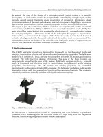
6. An illustrative example
Consider the model of a DC motor given by:
1

0
1
mt
a
a
ma
dw k
i
dt J J
di
R
wiu
dt L L L
τ
λ
=−
=− − +

where
a
i is the armature current,
m
w is the shaft speed, R is armature resistance,
o
λ

is the back-EMF constant,
1
τ
is the load torque, u is the terminal voltage, J is the inertia

of the motor, rotor and load, L is the armature inductance and
t
k is the torque constant.
Defining
1 m
x
w= and
2
,
a
x
i= and assuming that
1
τ
is a known constant we have:
1
1
2
0
2
0
0
1
0
t
k
x
x
J
u

J
x
R
x
L
LL
wSw
τ
λ
•
•
•
⎡⎤
⎡
⎤
⎡⎤
⎡⎤
⎢⎥
−
⎡⎤
⎢
⎥
⎢⎥
⎢⎥
=++
⎢⎥
⎢⎥
⎢
⎥
⎢⎥

⎢⎥
⎢⎥⎣⎦
−−
⎣⎦
⎣⎦
⎣
⎦
⎢⎥
⎣⎦
=

A Sampled-data Regulator using Sliding Modes and Exponential Holder for Linear Systems

245
where
()
123
,, ,
T
wwww=
000
00 ,
00
S
α
α
⎡
⎤
⎢
⎥

=
⎢
⎥
⎢
⎥
−
⎣
⎦

1, 2
,
ref
y
xy w==
11
w
τ
=
and
1,LmH= 0.5 ,R =Ω
2
0.001 ,JKgm=
1
0.001 ,
o
Vsrad
λ
−
=××
1

0.01 ,Nm s rad
β
−
=××
1
0.008 .
t
kNmA
−
=

From this, we can calculate
2
01 2
012
010
001, 0, , 0.aa a
aaa
α
⎡⎤
⎢⎥
Φ= = = =
⎢⎥
⎢⎥
−−−
⎣⎦

Discretizing the system with a sampling of
T=0.3 s and choosing a reference
0.1sin(5 )

ref
y
t= , the discrete robust controller with no exponential holder is
constructed with:
0.5399 1.0201 0 0 0
0.0645 0.1218 0 0 0
0.8072001 0
1.3671 0 0 0 1
1.3775 0 1 1.1414 1.1414
d
F
−
⎡
⎤
⎢
⎥
−
⎢
⎥
⎢
⎥
=
−
⎢
⎥
⎢
⎥
⎢
⎥
−

⎣
⎦

[
]
1.802 0.1481 0.8072 1.3671 1.3775
T
d
G =−−

where
[]
[][][]
0.9996 2.2284
0.1194 1 ,
0.00027 0.8603
0.343 0.279 , 1 0 , 1 0 0

dd
T
dd
A
BCH
⎡⎤
Σ= =
⎢⎥
−
⎣⎦
===

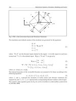
As is shown in Figure 1, as expected for the Discrete Sliding Regulator, the output tracking
error is zero at the sampling instant, but different from zero in the intersampling times.
Constructing now the controller (33) with an exponential holder we obtain
[
]
1.802 0.156 1.199 0.992 35.054
T
d
G =−−
Systems, Structure and Control

246
0.531 1.0201 0 0 0
0.0634 0.1218 0 0 0
1.1993 0 1 0.1994 0.0371
0.9922 0 0 0.0707 0.1994
35.0536 0 0 4.9874 0.0707
d
F
−
⎡
⎤
⎢
⎥
−
⎢
⎥
⎢
⎥
=

−
⎢
⎥
⎢
⎥
⎢
⎥
−
⎣
⎦

where
1 0.2sin(5 ) 0.04cos(5 ) 0.04
0 cos(5 ) 0.2sin(5 )
0 5sin(5 ) cos(5 )
e
θ
θθ
θθ
θθ
Φ
−+
⎡
⎤
⎢
⎥
=
⎢
⎥
⎢

⎥
−
⎣
⎦


Figure 1. Output tracking error for the Discrete Sliding Robust Regulator
As shown in Figure 2, the sliding discretized controller with exponential holder present a
remarkable performance guaranteeing zero output trackin error also in the intersampling.
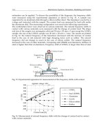
Finally, variations on the values of the parameters ranging up to
25%±
for R and
12%±
for L were introduced. As may be observed in Figure 3, the controller is able to
cope with these variations, maintaining the asymptotic tracking property as well.
A Sampled-data Regulator using Sliding Modes and Exponential Holder for Linear Systems

247

Figure 2. Output tracking error for the Ripple-Free Slidng Robust Regulator

Figure 3. Output tracking error for the Ripple-Free Slidng Robust Regulator with parametric
variations
7. Conclusions
In this paper, we presented an extensión to the Continuous Sliding Robust Regulator to the
Dicrete case. A Ripple-Free Sliding Robust Regulator which guarantees that the output
Systems, Structure and Control

248
tracking error is zeroed not only at the sampling instants, but also in the intersampling

behavior was alsoformulated and a solution was obtained. The controller has two
components: one of them depending of the discrete dynamics of the system, and the other
containing the internal model of the reference and/or perturbations generator. This feature
allows the implementation of the controller on a digital device. An illustrative example
shows the performance of the presented scheme.
8. Bibliography
Isidori, A., (1995), Nonlinear Control System. Third Edition. Ed. Springer-Verlag. [1]
Francis, B. A. and Wonham, W. M., (1976), The internal model principle of control theory.
Automatica. Vol. 12. pp. 457-465. [2]
Francis, B.A. (1977), The linear multivariable regulator problem. SIAM J. Control Optimiz., Vol.
15, pp. 486-505. [3]
Yung-Chun, W., Nie-Zen, Y. (1994). A Ripple Free Sampled-Data Robust Servomechanism
Controller Using Exponential Hold. IEEE Transactions on Automatic Control, Vol. 39,
No. 6, pp. 1287-1291. [4]
Franklin, G. F. & Emami-Naeini, A. (1986), Design of Ripple Free Multivariable Robust
Servomechanism, IEEE Trans. Aut. Control, Vol. AC-31, No. 7, pp. 661-664. [5]
Castillo-Toledo, B., Di Gennaro, S., Monaco, S. & Normand-Cyrot (1997), On regulation under
sampling, EEE Trans. Aut. Control, Vol. 42, No. 6, pp. 864-868. [6]
Kabamba, P. T. (1987), Control of Linear Systems using generalized sample-data hold funtions,
IEEE Trans. Aut. Control, Vol. AC-32, No. 9, pp. 772-782. [7]
Loukianov, Alexander G., Castillo-Toledo, B. and García, R. (1999) , Output Regulation in
Sliding Mode , Proc.of the American Control Conference, pp. 1037-1041. [8]
Castillo-Toledo, B., and Di Gennaro, S. (2002), On the nonlinear ripple free sampled-data
robust regulator. Eur. J. of Contr., Vol. 8, pp. 44- 55. [9]
Castillo-Toledo, B., and Obregon-Pulido, G. (2003). Guaranteeing asymptotic zero
intersampling tracking error via a discretized regulator and exponential holder for
nonlinear systems, J. App. Reserch & Tech. 1, pp. 203-214. [10]
Yamamoto, A., A function space approach to sampled data control systems and tracking
problems, IEEE Trans Aut. Control (1994); 350(4), pp 703-712 [11]
Utkin, V.I. (1981), Sliding modes in control and optimization (in Russian), Nauka. Moscow. [12]

Loukianov, A , Castillo-Toledo, B. and García, R. (1999) , On the sliding mode regulator
problem, Proc. of the 14th IFAC World Congress, pp. 61-66. [13]
Utkin V., Castillo-Toledo B., Loukianov A., Espinoza-Guerra O.(2002), On robust VSS
nonlinear servomechanism problem, in Variable Structure Systems: Towards the 21st
Century, Springer Verlag, Lecture Notes in Control and Information Scie ncies, vol. 274,
Berlín, , X. Yu and J-X. Xu Eds., pp. 343-363. ISBN 3 540 42965 4 [14]
V. Utkin, A. Loukianov , Castillo-Toledo B., , and J. Rivera (2004), Sliding mode regulador
design, in Variable Structure Systems: from Principles to implementation, The
Institution of Electrical Engineers, IEE Control Engineering Series, vol. 66, Sabanovi A.,
Fridman L and Spurgeon S. Eds., , pp. 19-44, ISBN 0 86341 350 1 [15]
El-Chesawi, O.M.E., Zinober, A.S.I., Billings, S.A. (1983), Analysis and design of variable
structure systems using a geometric approach. International Journal of Control 38, pp.
657-671. [16]