Supply Chain, The Way to Flat Organisation Part 11 doc
Bạn đang xem bản rút gọn của tài liệu. Xem và tải ngay bản đầy đủ của tài liệu tại đây (792.22 KB, 30 trang )
Distributed Supply Chain Planning for Multiple Companies with Limited Local Information
291
∑∑ ∑∑
∈∈
−+−=
Pit Pit
b
ti
a
ti
a
titi
a
a
SSrSλfL ||)(
,,,,
'
(22)
The penalty parameter r for a linear penalty term is gradually increased in each iteration. By
applying the linear approximation technique around a tentative solution for the proposed
method, the solutions derived by solving subproblem for each company cannot provide an
exact lower bound of the original problem.
3.4 Coordination of supply chain planning among multiple companies
A sequence of optimization problems
0
k
E can be given by (23) where
L
is given by (14).
0
()
k
E
'2
,,
'
min ( | | )
SC
cc
kit it
cZ c Z
Lr S S
∈∈
+−
∑∑
(23)
The decomposed subproblem for each company is reformulated as (24) and (25) by applying
the first order Taylor series of expansion around a tentative solution.
For supplier company
S
cZ
∈
0
()
k
c
EP
{
}
''
,,, ,, , , ,
'/{} '
min ( , , ) | |
SC
cc c c c c c c
it it it it it k it it it
iP t iP t c Z c cZ
f
SXY S r S S S
λ
∈∈∈∈
−+ + −
∑∑ ∑∑ ∑ ∑
(24)
For vendor company
C
dZ
∈
0
()
k
c
EP
{
}
''
,,, ,, , , ,
'/{} '
min ( , , ) | |
CS
dd d d d d c c
it it it it it k it it it
iP t iP t c Z d c Z
f
SXY S r S S S
λ
∈∈∈∈
++ + −
∑∑ ∑∑ ∑ ∑
(25)
subject to (1), (4)-(11)
The subproblem for each company is an MILP problem, which can be solved by a
commercial solver. r
k
represents a weighting factor for penalty function. To derive near-
optimal solution for the proposed method, the weighting factor r
k
must be gradually
increased according to the following equation.
rΔrr
kk
+
=
+1
(26)
Δ r is the step size parameter for penalty weighting coefficient which should be determined
by preliminary tests. Even though the objective function includes a linear penalty function
for each subproblem, a lower bound of the original problem can be obtained by calculating
L for the solution of subproblem when r
k
is set to zero.
3.5 Scenario of planning coordination for multiple companies
The system generates near-optimal plan in the following steps.
Step 1: Initialization
0k ← . The multipliers
,it
λ
and the weighting factor r
k
are set to an initial value (e.g. set
to zero).
Step 2: Generation of an initial plan
A manager for each company inputs the demanded delivery/receiving plan at each
time period
,
c
it
D and the total delivery/receiving quantity for each product during time
horizon. Each company solves each subproblem and generates a tentative plan with the
fixed multipliers.
Supply Chain, The Way to Flat Organisation
292
Step 3: Data exchange of tentative solution
Each company exchanges the data of tentative delivery/receiving quantity of products
c
ti
S
,
derived at each company.
Step 4: Evaluating the convergence
If the plan generated at Step 6 or Step 2 for initial iteration satisfies the following
conditions, the algorithm is considered as convergence. Then no more calculation is
made and the derived plan is regarded as a final plan.
i. The solution derived at Step 6 is the same as that generated at Step 6 in a previous
iteration.
ii. The solution derived at Step 6 satisfies the constraints (3).
iii. The solutions of all other companies also satisfy both of conditions (i) and (ii).
Step 5: Update of the multiplier and the weighting factor
The weighting factors are updated by (26) and the multipliers are updated by (18).
Step 6: Solving subproblems
A company solves its subproblem while the solution of other company is fixed. Then, the
tentative solution
c
ti
S
,
is updated and return to Step 3. If some of the companies derive its
solutions concurrently in parallel at Step 6, the same solution is generated cyclically because
tentative solution of a previous iteration is used, that makes the convergence of the
algorithm more difficult. Skipping heuristic (Nishi et al., 2002) is effective to avoid such
situations. Skipping heuristic is a procedure that the Step 6 for each company is randomly
skipped. If the proposed method is implemented on a parallel processing system, the
procedure must be added to avoid cyclic generation of solutions. Our numerical
experiments used a sequential computation that the Step 6 for each company is sequentially
executed to avoid the difficulty of convergence without skipping heuristic.
The data exchanged among companies is tentative supply and demand quantity in each
time period. This information is not directly concerned with confidential information for
each company. The multipliers are updated by (27) without using the information of
L
L−
for the step size because the upper bound is not calculated for augmented Lagrangian
approach.
⎪
⎪
⎩
⎪
⎪
⎨
⎧
∈∈=
∈∈>−
∈∈<+
=
)';()(
)';()(
)';()(
'
,,
*
,
'
,,
*
,
'
,,
*
,
,
CS
c
ti
c
titi
CS
c
ti
c
titi
CS
c
ti
c
titi
ti
ZcZcSSλ
ZcZcSSλΔλ
ZcZcSSλΔλ
λ
(27)
c
ti
S
,
represents a tentative solution obtained by solving subproblem for company
c
.
λΔ
is
the step size given as a scalar parameter, and
*
,ti
λ is the value of multipliers at a previous
iteration. For the proposed system,
λ
Δ
is considered as a constant step size without
generation of a feasible solution for the entire company. All of the information that is
exchanged at each iteration during the optimization is the tentative delivery quantity
}){\'(
'
,
cZZcS
CS
c
ti
∪∈ derived at other companies. Each company has the same value of
its own multipliers and updates the value of them for itself. Thus the dual problem can be
Distributed Supply Chain Planning for Multiple Companies with Limited Local Information
293
solved in a distributed environment without exchanging such confidential data as cost
information for the proposed method.
4. Computational experiments
4.1 Supply chain planning for 1 supplier and 2 vendor companies
An example of supply chain planning problem for 1 supplier (A) and 2 vendor companies
(B, C) treating with 2 types of products is solved. The total time horizon is 30 time periods.
The parameters for the problem are generated by random numbers on uniform distribution
in the interval shown in Table 1. The demanded delivery/receiving plan which is input data
for each company is illustrated in Fig. 1. The result obtained by the proposed method is also
shown in Fig. 2. The numbers printed in the figure indicate the delivery and receiving
quantity for each company. The program is coded by C++ language. A commercial MILP
solver, CPLEX8.0 ILOG(C) is used to solve subproblems. A Pentium IV 2AGHz processor
with 512 MB memory was used for computation.
The optimality of solution is minimized when
0.01r
Δ
= and 0.1
λ
Δ
= from several
preliminary tests. These parameters are used for computation in the following example
problems.
Supplier company
S
cZ
∈
Vendor company
C
cZ∈
,
c
it
D
0 – 200 0 – 180
,
c
it
μ
1 – 10 1 – 10
,
c
it
d
1 – 10 1 – 10
c
i
e
10 – 30 10 – 30
,
c
it
m
1500 – 4000 750 – 2000
Table 1. Parameters for the example problems
Augmented Lagrangian decomposition method ( ALDC )
0.1
λ
Δ
= , 0.01r
Δ
=
Lagrangian decomposition method ( LDC )
0.1
γ
=
Penalty method ( PM )
0.01r
Δ
= (Case 1, Case 2), 0.1r
Δ
= (Case 3)
Table 2. Parameters for the distributed optimization method
I
t
e
m
#
1
Ite
m
#2
Time period [term]
Supplier A
Vendor B
Vendor C
Fig. 1. An initial request for the plan ( 1 supplier and 2 vendor companies)
Supply Chain, The Way to Flat Organisation
294
I
t
e
m
#1 Ite
m
#
2
Time period [term]
Supplier A
Vendor B
Vendor C
Fig. 2. Result of distributed supply chain planning by the proposed method (after 72 times
of data exchanges)
Time period [term]
I
t
e
m
#1 Ite
m
#2
Supplier A
Vendor B
Vendor C
Fig. 3. The optimal solution derived by CPLEX solver
The proposed method generates a feasible solution for the problem after 72 iterations using
the parameters shown in Table 2. The result is shown in Fig. 2. An optimal solution derived
by commercial solver is also shown in Fig. 3. The result obtained by the proposed method is
almost the same as that of an optimal solution. The transition of the value of L
r
and the
decomposed function
'
r
L
for each company c is shown in Fig. 4. The condition for
evaluating convergence is that the difference of the delivery and receiving quantity is less
than 0.01 for all products and for all time periods. The optimal value of the objective
function of (2) obtained by the proposed method is 9,979. The value for the optimal solution
obtained by the commercial MILP solver with all of the information is 9,960. The gap
between the derived solution and the optimal solution is 0.18%. It demonstrates that the
proposed method can derive near-optimal solution without requiring all of the information
for other companies.
0
2000
4000
6000
8000
10000
1
2
0
0
0
1 6 11 16 21 26 31 36 41 46 51 56 61 66 71
Iteration [-]
Value of objective function [-]
Vendor B
Vendor C
Supplier A
augmented Lagrangian function
linear penalty function
optimal solution
Fig. 4. Transition of the value of objective function for the proposed method
Distributed Supply Chain Planning for Multiple Companies with Limited Local Information
295
4.2 Comparison with other distributed optimization methods
To investigate the performance of the proposed method, the performance of the proposed
method (ALDC method) is compared with other distributed optimization methods: a
penalty method (PM method) that the terms of Lagrangian multipliers are removed from
(24) and (25), and an ordinary LDC method (LDC method).
For the LDC method, the dual problem D
0
is solved by standard Lagrangian function. The
dual solution is modified to generate a feasible solution with the following heuristic
procedure at each iteration. The heuristic procedure is constructed so that the constraint
violation is checked in forward and the solution is modified to satisfy three types of
constraints of (5), (6), (7) and (8), (9) successively satisfying (3).
Step i) Receiving quantity for vendor companies is modified to satisfy the delivery quantity
for suppliers. Set
).,,1;;(
);,,1;;(
,,
,,
HtPiZdS
m
m
S
HtPiZcSS
C
S
Zc
c
ti
C
Zy
d
i
d
i
d
ti
S
c
ti
c
ti
…
…
=∀∈∀∈∀←
=∀∈∀∈∀←
∑
∑
∈
∈
Step ii) Find a time period t in forward in which (5) is violated. For a plan in time period t,
one type of product is allocated and allocation of other types of products are moved to a
neighbour time period e.g. (t -1) or (t +1). If (3) and (5) are not satisfied, then return to step i).
Otherwise go to step iii).
Step iii) Find a time period t in forward in which (6) or (7) is violated. For a plan in time
period t, the violated delivery/receiving quantity is modified to allocate into a neighbour
time period e.g. (t -1) or (t +1). If (3) and (5)-(7) are not satisfied, then return to step i).
Otherwise go to step iv).
Step iv) Find a time period t in forward when (8) or (9) is violated. For a plan in time period
t, the allocation of delivery/receiving quantity is modified to allocate a neighbour time
period e.g. (t -1) or (t +1). If (3) and (5)-(9) are not satisfied, return to step i). Otherwise the
heuristic procedure is completed.
Three cases of the supply chain planning problem for 1 supplier and 2 vendor companies
are solved by the proposed method, LDC method and PM method. For each case, ten types
of problems are generated by using random numbers on uniform distribution with different
seeds in the range shown in Table 1. The parameters used for each method are shown in
Table 2. The average objective function (Ave. obj. func.), average gap between the solution
and an optimal solution (Ave. gap), average number of iterations to converge (Ave. num.
iter.), and average computation time (Ave. comp. time) for ten times of calculations for each
case are summarized in Table 3. The centralized MILP method uses a branch and bound
method to obtain an optimal solution by CPLEX 8.0 using Pentium IV 2GHz processor with
512MB memory.
Computational results of Table 3 show that the ALDC method can generate better solutions
than any other distributed optimization methods. The gap between the optimal solutions is
within 3% for all cases. This indicates that the proposed method can generate near-optimal
solution without using the entire information for each company. The total computation time
for ALDC method to derive a feasible solution is shorter than that of MILP method,
however, it is larger than that of PM method. The MILP solver cannot derive a solution
Supply Chain, The Way to Flat Organisation
296
within 100,000 seconds of computation time for Case 3 (3 types of products). This is why the
computational complexity for the problem grows exponentially with number of products.
The petroleum complex usually treats multi-products more than 3 types of products. Thus it
is very difficult to apply the conventional MILP solver for supply chain planning for
multiple companies. The optimality performance of the LDC method is not better than the
other methods. This is because the heuristic procedure to generate a feasible solution is not
effective for large-sized problems. The LDC method cannot derive a feasible solution by the
current heuristic procedure. This is due to the difficulty of finding a feasible solution to
satisfy all of such constraints as setup time constraints, and delivery duration constraints.
The computation time of penalty method (PM method) is shorter than the proposed
method, however, the optimality performance is not better than that of the proposed
method. This result implies that the use of Lagrangian multipliers is effective to improve the
optimality performance. Even though the proposed method needs a number of iterations to
converge to a feasible solution than that of PM method, it is demonstrated that near-optimal
solution with less than 3% of gap from the optimal solution can be obtained by the proposed
method.
Case 1 Problem for 1 type of product
Method MILP ALDC LDC PM
Ave. obj. func. [-] 10,829 10,976 13,297 11,153
Ave. gap [%] 0.00 1.37 23.0 2.90
Ave. num. iter. - 180 90 53
Ave. comp. time[s] 1783 110 85 27
Case 2 Problem for 2 types of products
Method MILP ALDC LDC PM
Ave. obj. func. [-] 48,700 49,975 50,562 51,005
Ave. gap [%] 0.00 2.71 4.06 4.66
Ave. num. iter. - 137 80 39
Ave. comp. time[s] 16,142 246 149 41
Case 3 Problem for 3 types of products
Method MILP ALDC LDC PM
Ave. obj. func. [-] - 78280 - 79089
Ave. num. iter. - 827 - 104
Ave. comp. time[s] - 110 - 30
Table 3. Comparison of the performances of MILP and the distributed optimization methods
5. Conclusion and future works
A distributed supply chain planning system for multiple companies using an augmented
Lagrangian relaxation method has been proposed. The original problem is decomposed into
several sub-problems. The proposed system can derive a near optimal solution without
using the entire information about the companies. By using a new penalty function, the
proposed method can obtain a feasible solution without using a heuristic procedure. This is
also a predominant characteristic of the proposed algorithm and the improvement of the
conventional Lagrangian relaxation methods. It is demonstrated from numerical tests that a
near optimal solution within a 3% of gap from an optimal solution can be obtained with a
Distributed Supply Chain Planning for Multiple Companies with Limited Local Information
297
reasonable computation time. The applicability of the augmented Lagrangian function to the
various class of supply chain planning problems is one of our future works.
6. References
Androulakis, I.P. & Reklaitis, G.V. (1999). Approaches to Asynchronous Decentralized
Decision Making, Computers and Chemical Engineering, Vol. 23, pp. 341-355.
Beltan, C. & Herdia, F.J. (1999). Short-Term Hydrothermal Coordination by Augmented
Lagrangean Relaxation: a new Multiplier Updating, Investigaci\'on Operativa, Vol.
8, pp. 63-76.
Beltran, C. & Heredia, F.J. (2002). Unit Commitment by Augmented Lagrangian Relaxation:
Testing Two Decomposition Approaches, Journal of Optimization Theory and
Application, Vol. 112, No. 2, pp. 295-314.
Bertsekas, D.P. (1976). Multiplier Methods: A Survey, Automatica, Vol. 12, pp. 133-145.
Cohen, G. & Zhu D.L. (1984) Decomposition Coordination Methods in Large Scale
Optimization Problems: the nondifferentiable case and the use of augmented
Lagrangians, Advances in Large Scales Systems, vol. 1, pp. 203-266.
Fisher, M.L. (1973). The Lagrangian Relaxation Method for Solving Integer Programming
Problems, Management Science, vol. 27, no. 1, pp. 1-18.
Gaonkar, R. & Viswanadham, N. (2002). Integrated Planning in Electronic Marketplace
Embedded Supply Chains, Proceedings of IEEE International Conference on Robotics
and Automation, pp. 1119-1124.
Georges, D. (1994). Optimal Unit Commitment in Simulations of Hydrothermal Power
Systems: An Augmented Lagrangian Approach, Simulation Practice and Theory, vol.
1, pp. 155-172.
Gupta, A. & Maranus, C.D. (1999) Hierarchical Lagrangian Relaxation Procedure for Solving
Midterm Planning Problems, Industrial Engineering and Chemistry Research, vol. 38,
pp. 1937-1947.
Hoitomt, D.J., Luh, P.B. & Pattipati, K.R. (1993) A Practical Approach to Job-Shop
Scheduling Problems, IEEE Transactions on Robotics and Automation, vol. 9, no. 1, pp.
1-13.
Jackson, J.R. & Grossmann, I.E. (2003) Temporal Decomposition Scheme for Nonlinear
Multisite Production Planning and Distribution Models, Industrial Engineering and
Chemistry Research, vol. 42, pp. 3045-3055.
Jayaraman, V. & Pirkul, H. (2001) Planning and Coordination of Production and
Distribution Facilities for Multiple Commodities, European Journal of Operational
Research, vol. 133, pp. 394-408.
Julka, N., Srinivasan, R. & Karimi, I. (2002) Agent-based Supply Chain Management,
Computers and Chemical Engineering, vol. 26, pp. 1755-1769.
Luh, P.B. & Hoitomt, D.J. (1993) Scheduling of Manufacturing Systems Using the
Lagrangian Relaxation Technique, IEEE Transactions on Automatic Control, vol. 38,
no. 7, pp. 1066-1079.
Luh, P.B., Ni, M., Chen, H. & Thakur, L.S. (2003) Price-Based Approach for Activity
Coordination in a Supply Network, IEEE Transactions on Robotics and Automation,
vol. 19, No. 2, pp. 335-346.
Supply Chain, The Way to Flat Organisation
298
McDonald, C.M. & Karimi, I.A. (1997) Planning and Scheduling of Parallel Semicontinuous
Processes. 1. Production Planning, Industrial Engineering and Chemistry Research, vol.
36, pp. 2691-2700.
Nishi, T., Konishi, M., Hasebe, S. & Hashimoto, I. (2002) Machine Oriented Decentralized
Scheduling Method using Lagrangian Decomposition and Coordination Technique,
Proceedings of IEEE International Conference on Robotics and Automation, pp. 4173-
4178.
Rockafellar, R.T. (1974) Augmented Lagrange Multiplier Functions and Duality in
Nonconvex Programming, SIAM Journal of Control, vol. 12, no. 2, pp. 269-285.
Stephanopoulos, G. & Westerberg, A.W. (1975) The Use of Hestenes' Method of Multipliers
to Resolve Dual Gaps in Engineering System Optimization, Journal of Optimization
Theory and Application, vol. 15, no. 3, pp. 285-309.
Taneda, D. (2003) Approach to the Advanced Refining and Petro Chemical Complexes,
Chemical Engineering Journal, vol. 67, no. 3, pp. 46-183 (in Japanese).
Tu, Y., Luh, P.B., Feng, W., & Narimatsu, K. (2003) Supply Chain Performance Evaluation: A
Simulation Study, Proceedings of IEEE International Conference on Robotics and
Automation, pp. 1749-1755.
Vidal, C. J. & Goetshalckx, M. (1997) Strategic Production-distribution Models: A Critical
Review with Emphasis on Global Supply Chain Models, European Journal of
Operational Research, vol. 98, no. 1, pp. 1-18.
16
Applying Fuzzy Linear Programming to
Supply Chain Planning with Demand,
Process and Supply Uncertainty
David Peidro, Josefa Mula and Raúl Poler
Research Centre on Production Management and Engineering (CIGIP)
Universidad Politécnica de Valencia,
SPAIN
1. Introduction
A Supply Chain (SC) is a dynamic network of several business entities that involve a high
degree of imprecision. This is mainly due to its real-world character where uncertainties in
the activities extending from the suppliers to the customers make SC imprecise (Fazel
Zarandi et al., 2002).
Several authors have analysed the sources of uncertainty present in a SC, readers are
referred to Peidro et al. (2008) for a review. The majority of the authors studied
(Childerhouse & Towill, 2002; Davis, 1993; Ho et al., 2005; Lee & Billington, 1993; Mason-
Jones & Towill, 1998; Wang & Shu, 2005), classified the sources of uncertainty into three
groups: demand, process/manufacturing and supply. Uncertainty in supply is caused by
the variability brought about by how the supplier operates because of the faults or delays in
the supplier’s deliveries. Uncertainty in the process is a result of the poorly reliable
production process due to, for example, machine hold-ups. Finally, demand uncertainty,
according to Davis (Davis, 1993), is the most important of the three, and is presented as a
volatility demand or as inexact forecasting demands.
The coordination and integration of key business activities undertaken by an enterprise,
from the procurement of raw materials to the distribution of the end products to the
customer, are concerned with the SC planning process (Gupta & Maranas, 2003), one of the
most important processes within the SC management concept. However, the complex
nature and dynamics of the relationships among the different actors imply an important
degree of uncertainty in the planning decisions. In SC planning decision processes,
uncertainty is a main factor that can influence the effectiveness of the configuration and
coordination of supply chains (Davis, 1993; Jung et al., 2004; Minegishi & Thiel, 2000) and
tends to propagate up and down along the SC, affecting its performance appreciably
(Bhatnagar & Sohal, 2005).
Most of the SC planning research (Alonso-Ayuso et al., 2003; Guillen et al., 2005; Gupta y
Maranas, 2003; Lababidi et al., 2004; Santoso et al., 2005; Sodhi, 2005) models SC
uncertainties with probability distributions that are usually predicted from historical data.
However, whenever statistical data are unreliable or are even not available, stochastic
models may not be the best choice (Wang y Shu, 2005). The fuzzy set theory(Zadeh, 1965)
Supply Chain, The Way to Flat Organisation
300
and the possibility theory (Dubois & Prade, 1988; Zadeh, 1978) may provide an alternative
simpler and less-data demanding then probability theory to deal with SC uncertainties
(Dubois et al., 2003).
Few studies address the SC planning problem on a medium-term basis (tactical level) which
integrate procurement, production and distribution planning activities in a fuzzy
environment (see Section 2. Literature review). Moreover, models contemplating the
different sources of uncertainty in an integrated manner are lacking. Hence in this study, we
develop a tactical supply chain model in a fuzzy environment in a multi-echelon, multi-
product, multi-level, multi-period supply chain network. In this proposed model, the
demand, process and supply uncertainties are contemplated simultaneously.
In the context of fuzzy mathematical programming, two very different issues can be
addressed: fuzzy or flexible constraints for fuzziness, and fuzzy coefficients for lack of
knowledge or epistemic uncertainty (Dubois et al., 2003). Our proposal jointly considers the
possible lack of knowledge in data and existing fuzziness.
The main contributions of this paper can be summarized as follows:
• Introducing a novel tactical SC planning model by integrating procurement, production
and distribution planning activities into a multi-echelon, multi-product, multi-level and
multi-period SC network.
• Achieving a model which contemplates the different sources of uncertainty affecting
SCs in an integrated fashion by jointly considering the possible lack of knowledge in
data and existing fuzziness.
• Applying the model to a real-world automobile SC dedicated to the supply of
automobile seats.
The rest of this paper is arranged as follows. Section 2 presents a literature review about
fuzzy applications in SC planning. Section 3 proposes a new fuzzy mixed-integer linear
programming (FMILP) model for the tactical SC planning under uncertainty. Then in
Section 4, appropriate strategies for converting the fuzzy model into an equivalent auxiliary
crisp mixed-integer linear programming model are applied. In Section 5, the behaviour of
the model in a real-world automobile SC has been evaluated and, finally, the conclusions
and directions for further research are provided.
2. Literature review
In Peidro et al. (2008) a literature survey on SC planning under uncertainty conditions by
adopting quantitative approaches is developed. Here, we present a summary, extracted
from this paper, about the applications of fuzzy set theory and the possibility theory to
different problems related to SC planning:
SC inventory management
: Petrovic et al. (1998; 1999) describe the fuzzy modelling and
simulation of a SC in an uncertain environment. Their objective was to determine the stock
levels and order quantities for each inventory during a finite time horizon to achieve an
acceptable delivery performance at a reasonable total cost for the whole SC. Petrovic (2001)
develops a simulation tool, SCSIM, for analyzing SC behaviour and performance in the
presence of uncertainty modelled by fuzzy sets. Giannoccaro et al. (2003) develop a
methodology to define inventory management policies in a SC, which was based on the
echelon stock concept (Clark & Scarf, 1960) and the fuzzy set theory was used to model
uncertainty associated with both demand and inventory costs. Carlsson and Fuller (2002)
propose a fuzzy logic approach to reduce the bullwhip effect. Wang and Shu (2005) develop
Applying Fuzzy Linear Programming to Supply Chain Planning
with Demand, Process and Supply Uncertainty
301
a decentralized decision model based on a genetic algorithm which minimizes the inventory
costs of a SC subject to the constraint to be met with a specific task involving the delivery of
finished goods. The authors used the fuzzy set theory to represent the uncertainty of
customer demands, processing times and reliable deliveries. Xie et al. (2006) present a new
bilevel coordination strategy to control and manage inventories in serial supply chains with
demand uncertainty. Firstly, the problem associated with the whole SC was divided into
subproblems in accordance with the different parts that the SC it was made up of. Secondly,
for the purpose of improving the integrated operation of a whole SC, the leader level was
defined to be in charge of coordinating inventory control and management by amending the
optimisation subproblems. This process was to be repeated until the desired level of
operation for the whole SC was reached.
Vendor Selection
: Kumar et al. (2004) present a fuzzy goal programming approach which
was applied to the problem of selecting vendors in a SC. This problem was posed as a mixed
integer and fuzzy goal programming problem with three basic objectives to minimize: the
net cost of the vendors network, rejects within the network, and delays in deliveries. With
this approach, the authors used triangular membership functions for each fuzzy objective.
The solution method was based on the intersection of membership functions of the fuzzy
objectives by applying the min-operator. Then, Kumar et al. (2006a) solve the same problem
using the multi-objective fuzzy programming approach proposed by (Zimmermann, 1978).
Amid et al. (2006) address the problem of adequately selecting suppliers within a SC. For
this purpose, they devised a fuzzy-based multi-objective mathematical programming model
where each objective may be assigned a different weight. The objectives considered were
related to cost cuts, increased quality and to an increased service of the suppliers selected.
The imprecise elements considered in this work were to meet both objectives and demand.
Kumar et al. (2006b) analyze the uncertainty prevailing in integrated steel manufacturers in
relation to the nature of the finished good and the significant demand by customers. They
proposed a new hybrid evolutionary algorithm named endosymbioticpsychoclonal (ESPC)
to decide what and how much to stock as an intermediate product in inventories. They
compare ESPC with genetic algorithms and simulated annealing. They conclude the
superiority of the proposed algorithm in terms of both the quality of the solution obtained
and the convergence time.
Transport planning
: Chanas et al. (1993) consider several assumptions on the supply and
demand levels for a given transportation problem in accordance with the kind of
information that the decision maker has: crisp values, interval values or fuzzy numbers. For
each of these three cases, classical, interval and fuzzy models for the transportation problem
are proposed, respectively. The links among them are provided, focusing on the case of the
fuzzy transportation problem, for which solution methods are proposed and discussed. Shih
(1999) addresses the problem of transporting cement in Taiwan by using fuzzy linear
programming models. The author uses three approaches based on the works by
Zimmermann (1976). Chanas (1983) and Julien (1994), who contemplate: the capacities of
ports, the fulfilling demand, the capacities of the loading and unloading operations, and the
constraints associated with traffic control. Liu and Kao (2004) develop a method to obtain
the membership function of the total transport cost by considering this as a fuzzy objective
value where the shipment costs, supply and demand are fuzzy numbers. The method was
based on the extension principle defined by Zadeh (1978) to transform the fuzzy transport
problem into a pair of mathematical programming models. Liang (2006) develops an
Supply Chain, The Way to Flat Organisation
302
interactive multi-objective linear programming model for solving fuzzy multi-objective
transportation problems with a piecewise linear membership function.
Production-distribution planning
: Sakawa et al. (2001) address the real problem of
production and transport related to a manufacturer through a deterministic mathematical
programming model which minimizes costs in accordance with capacities and demands.
Then, the authors develop a mathematical fuzzy programming model. Finally, they present
an outline of the distribution of profits and costs based on the game theory. Liang (2007)
proposes an interactive fuzzy multi-objective linear programming model for solving an
integrated production-transportation planning problem in supply chains. Selim et al. (2007)
propose fuzzy goal-based programming approaches applied to planning problems of a
collaborative production-distribution type in centralized and decentralized supply chains.
The fuzzy elements that the authors consider correspond to the fulfilment of different
objectives related to maximizing profits for manufacturers and distribution centers, retailer
cost cuts and minimizing delays in demand in retailers. Aliev et al. (2007) develop an
integrated multi-period, multi-product fuzzy production and distribution aggregate
planning model for supply chains by providing a sound trade-off between the fillrate of the
fuzzy market demand and the profit. The model is formulated in terms of fuzzy
programming and the solution is provided by genetic optimization.
Procurement-production-distribution planning
: Chen and Chang (2006) develop an
approach to derive the membership function of the fuzzy minimum total cost of the multi-
product, multi-echelon, and multi-period SC model when the unit cost of raw materials
supplied by suppliers, the unit transportation cost of products, and the demand quantity of
products are fuzzy numbers. Recently, Tarabi and Hassini (2008) propose a new multi-
objective possibilistic mixed integer linear programming model for integrating procurement,
production and distribution planning by considering various conflicting objectives
simultaneously along with the imprecise nature of some critical parameters such as market
demands, cost/time coefficients and capacity levels. The proposed model and solution
method are validated through numerical tests.
As mentioned before, models contemplating the different sources of uncertainty in an
integrated manner are lacking and few studies address the SC planning problem on a
medium-term basis which integrate procurement, production and distribution planning
activities in a fuzzy environment. Moreover, the majority of the models studied are not
applied in supply chains based on real world cases.
3. Problem description
This section outlines the tactical SC planning problem. The overall problem can be stated as
follows:
Given:
- A SC topology: number of nodes and type (suppliers, manufacturing plants,
warehouses, distribution centers, retailers, etc.)
- Each cost parameter, such as manufacturing, inventory, transportation, demand
backlog, etc.
- Manufacture data, processing times, production capacity, overtime capacity, BOM,
production run, etc.
- Transportation data, such as lead time, transport capacity, etc.
- Procurement data, procurement capacity, etc.
Applying Fuzzy Linear Programming to Supply Chain Planning
with Demand, Process and Supply Uncertainty
303
- Inventory data, such as inventory capacity, etc.
- Forecasted product demands over the entire planning periods.
To determine:
- The production plan of each manufacturing node.
- The distribution transportation plan between nodes.
- The procurement plan of each supplier node.
- The inventory level of each node.
- The sales and demand backlog.
The target is to centralize the multi-node decisions simultaneously in order to achieve the
best utilization of the resources available in the SC throughout the time horizon so that
customer demands are met at a minimum cost.
3.1 Fuzzy model formulation
The fuzzy mixed integer linear programming (FMILP) model for the tactical SC planning
proposed by Peidro et al. (2007) is adopted as the basis of this work. Sets of indices,
parameters and decision variables for the FMILP model are defined in the nomenclature
(see Table 1). Table 2 shows the uncertain parameters grouped according to the uncertainty
sources that may be presented in a SC.
Set of indices
T:
Set of planning periods (t =1, 2…T).
I:
Set of products (raw materials, intermediate products, finished goods) (i =1,
2…I).
N:
Set of SC nodes (n =1, 2…N).
J:
Set of production resources (j =1, 2…J).
L:
Set of transports (l =1, 2…L).
P:
Set of parent products in the bill of materials (p =1, 2…P).
O:
Set of origin nodes for transports (o =1, 2…O).
D:
Set of destination nodes for transports (d =1, 2…D).
Objective function cost coefficients
injt
CPV
~
:
Variable production cost per unit of product i on j at n in t.
njt
CTO
~
:
Overtime cost of resource j at n in t.
njt
CTU
~
:
Undertime cost of resource j at n in t.
RMC
int
:
Price of raw material i at n in t.
odlt
CT
~
:
Transport cost per unit from o to d by l in t.
int
CI
~
:
Inventory holding cost per unit of product i at n in t.
int
CBD
~
:
Demand backlog cost per unit of product i at n in t.
General Data
B
pint
:
Quantity of i to produce a unit of p at n in t.
nt
CRMP
~
:
Maximum procurement capacity from supplier node n in t.
int
D
~
:
Demand of product i at n in t.
njt
TOM
~
:
Overtime capacity of resource j at n in t.
njt
CPM
~
:
Production capacity of resource j at n in t.
Supply Chain, The Way to Flat Organisation
304
I0
in
:
Inventory amount of i at n in period 0.
PR
injt
:
Production run of i on j at n in t.
MPR
injt
:
Minimum production run of i on j at n in t.
DB0
int
:
Demand backlog of i at n in period 0.
SR0
iodlt
:
Shipments of i received at d from o by l at the beginning of period 0.
SIP0
iodlt
:
Shipments in progress of i from o to d by l at the beginning of period 0.
injt
TP
~
:
Processing time to produce a unit of i on j at n in t.
odlt
TLT
~
:
Transport lead time from o to d by l in t.
V
it
:
Physical volume of product i in t.
nt
CTM
~
:
Maximum transport capacity of l in t.
nt
CIM
~
:
Maximum inventory capacity at n in t.
1
odlt
χ
:
0-1 function. It takes 1 if TLT
odlt
> 0 and 0 otherwise.
2
odlt
χ
:
0-1 function. It takes 1 if TLT
odlt
= 0 and 0 otherwise.
Decision Variables
P
injt
:
Production amount of i on j at n in t / PT
injt
> 0.
k
injt
:
Number of production runs of i produced on j at n in t.
S
int
:
Supply of product i from n in t.
DB
int
:
Demand backlog of i at n in t / DBC
int
> 0.
TQ
iodlt
:
Transport quantity of i from o to d by l in t / o <> d, TC
odlt
> 0, IC
i,n=d,t
> 0.
SR
iodlt
:
Shipments of i received at d from o by l at the beginning of period t / o <> d,
TC
odlt
> 0, IC
i,n=d,t
> 0.
SIP
iodlt
:
Shipments in progress of i from o to d by l at the beginning of period t / o
<> d, TC
odlt
> 0, IC
i,n=d,t
> 0, TLT
odlt
> 0.
FTLT
iodlt
:
Transport lead time for i from o to d by l in t (only used in the fuzzy model).
I
int
:
Inventory amount of i at n at the end of period t.
PQ
int
:
Purchase quantity of i at n in t / RMC
int
> 0.
OT
njt
:
Overtime for resource j at n in t.
UT
njt
:
Undertime for resource j at n in t.
YP
injt
:
Binary variable indicating whether a product i has been produced on j at n
in t.
Table 1. Nomenclature (fuzzy parameters are shown with tilde: ~).
FMILP is formulated as follows:
Minimize z =
∑∑∑∑∑∑∑∑
∑∑∑∑∑∑∑
========
=======
⋅+⋅+⋅+⋅+
+⋅+⋅+⋅
I
i
O
o
D
d
L
l
T
t
iodltodltintintintint
I
i
N
n
T
t
intint
njtnjt
N
n
J
j
T
t
njtnjt
I
i
N
n
J
j
T
t
injtinjt
TQCTDBCBDICIPQRMC
UTCTUOTCTOPCPV
11111111
1111111
)
~
()
~
~
(
)
~~
()
~
(
(1)
Subject to
njtnjt
I
i
injtinjt
TOMCPMTPP
~
~
~
)
~
(
1
+≤⋅
∑
=
t j, n,
∀
(2)
Applying Fuzzy Linear Programming to Supply Chain Planning
with Demand, Process and Supply Uncertainty
305
Source of uncertainty in
supply chains
Fuzzy coefficient Formulation
Product demand
int
D
~
Demand
Demand backlog cost
int
CBD
~
Processing time
injt
TP
~
Production capacity
njtnjt
TOMCPM
~
,
~
Production costs
njtnjtinjt
CTUCTOCPV
~
,
~
,
~
Inventory holding cost
int
CI
~
Process
Maximum inventory
capacity
nt
CIM
~
Transport lead time
odlt
TLT
~
Transport cost
odlt
CT
~
Maximum transport
capacity
nt
CTM
~
Supply
Maximum procurement
capacity
nt
CRMP
~
Table 2. Fuzzy parameters considered in the model.
injtinjtinjt
PRkP
⋅
=
t j, n, i,
∀
(3)
injtnjtinjtnjtinjtinjt
YPTOMYPCPMPTP ⋅+⋅≤⋅
~
~
~
t j, n, i,
∀
(4)
injtinjtinjt
YPMPRP
⋅
≥
t j, n, i,
∀
(5)
∑∑∑∑
∑∑∑
==
=
==
=
===
=−
⋅−−−
−+++=
P
p
J
j
njtpipint
D
d
L
l
intdltnoi
J
j
O
o
L
l
intltndioinjttinint
PBSTQ
PQSRPII
11
,
11
,,
111
,,1,
)(
t n, i,
∀
(6)
TLTtiodl
iodltiodlt
TQSRSR
~
,
0
−
+
=
tldoi ,,,,
∀
(7)
iodltiodlttiodliodltiodlt
SRTQSIPSIPSIP
−
+
+
=
−1,
0
tldoi ,,,,
∀
(8)
ntit
I
i
int
CIMVI
~
~
1
≤⋅
∑
=
t n,
∀
(9)
ltit
I
i
O
o
D
d
iodltit
I
i
O
o
D
d
iodlt
CTMVTQVSIP
odltodlt
~
~
2
111
1
111
≤⋅⋅+⋅⋅
∑∑∑∑∑∑
======
χχ
t l,
∀
(10)
nt
I
i
int
CRMPPQ
~
~
1
≤
∑
=
t n,
∀
(11)
Supply Chain, The Way to Flat Organisation
306
intinttinint
SDDBDB −+≈
−
~
1,
t n, i,
∀
(12)
∑
=
+−⋅≈
I
i
njtnjtinjtinjtnjt
UTCPMTPPOT
1
~~
t j, n,
∀
(13)
(
)
∑∑∑∑
====
+≤
N
n
T
t
intint
N
n
T
t
int
DBDS
1111
0
~
~
i
∀
(14)
0, ≥
injtinjt
kP
t j, n, i,
∀
(15)
0,,, ≥
intintintint
PQIDBS
t n, i,
∀
(16)
0,, ≥
iodltiodltiodlt
TQSIPSR
tldoi ,,,,
∀
(17)
0, ≥
njtnjt
UTOT
t j, n,
∀
(18)
Eq. (1) shows the total cost to be minimized. The total cost is formed by the production costs
with the differentiation between regular and overtime production. The costs corresponding
to idleness, raw material acquisition, inventory holding, demand backlog and transport are
also considered. Most of these costs cannot be measured easily since they mainly imply
human perception for their estimation. Therefore, these costs are considered uncertain data
and are modelled by fuzzy numbers. Only the raw material cost is assumed to be known.
The production time per period could never be higher than the available regular time plus
the available overtime for a certain production resource of a node (2). Symbol
≤
~
represents
the fuzzy version of ≤ and means “essentially less than or similar to”. This constraint shows
that the planner wants to make the left-hand side of the constraint, the production time per
period, smaller or similar to the right-hand side, the maximum production time available,
“if possible”. The production time and the production capacity are only known
approximately and are represented by fuzzy numbers. On the other hand, the produced
quantity of each product in every planning period must always be a multiple of the selected
production lot size (3).
Eq. (4) and (5) guarantee a minimum production size for the different productive resources
of the nodes in the different periods. These equations guarantee that P
injt
will be equal to
zero if YP
injt
is zero.
Eq. (6) corresponds to the inventory balance. The inventory of a certain product in a node, at
the end of the period, will be equal to the inputs minus the outputs of the product generated
in this period. The inputs concern the production, transport receptions from other nodes,
purchases (if supplying nodes) and the inventory of the previous period. The outputs are
related to shipments to other nodes, supplies to customers and the consumption of other
products (raw materials and intermediate products) that are necessary to produce in the
node.
Eqs. (7) and (8) control the shipment of products among nodes. The receptions of shipments
for a certain product will be equal to the programmed receptions plus the shipments carried
out in previous periods. In constraint (7), the transport lead time are considered uncertainty
data. On the other hand (8), the shipments in progress will be equal to the initial shipments
Applying Fuzzy Linear Programming to Supply Chain Planning
with Demand, Process and Supply Uncertainty
307
in progress plus those from the previous period, plus the new shipments initiated in this
period minus the new receptions.
Both the transports and inventory levels are limited by the available volume (known
approximately). Thus according to Eq. (9), the inventory level for the physical volume of
each product must be lower than the available maximum volume for every period
(considered uncertainty data). The inventory volume depends on the period to consider the
possible increases and decreases of the storage capacity over time. Additionally, the physical
volume of the product depends on the time to cope with the possible engineering changes
that can occur and affect the dimensions and volume of the different products.
On the other hand, the shipment quantities in progress of each shipment in every period
multiplied by the volume of the transported products (if the transport time is higher than 0
periods), plus the initiated shipments by each transport in every period multiplied by the
volume of the transported products (if the transport time is equal to 0 periods), can never
exceed the maximum transport volume for that period (10). The reason for using a different
formulation in terms of the transport time among nodes (TLT
odlt
) is because the transport in
progress will never exist if this value is not higher than zero because all the transport
initiated in a period is received in this same period if TLT
odlt
= 0. Finally, the transport
volume depends on the period to consider the possible increases and decreases of the
transport capacity over time.
Eq. (11) establishes an estimated maximum of purchase for each node and product per
period. Eq. (12) contemplates the backlog demand management over time. The backlog
demand for a product and node in a certain period will be equal (approximately) to the
backlog demand of the previous period plus the difference between supply and demand.
Eq. (13) considers the use of overtime and undertime production for the different productive
resources. The overtime production for a productive resource of a certain node in one period
is equal (approximately) to the total production time minus the available regular production
time plus the idle time. OT
njt
and UT
njt
will always be higher or equal to zero if the total
production time is higher than the available regular production time, UT
njt
will be zero as it
does not incur in added costs, and OT
njt
will be positive. On the contrary, if the total
production time is lower than the available regular production time, UT
njt
will be positive
and OT
njt
will be zero.
Conversely, Eq. (14) establishes that the sum of all the supplied products is essentially lower
or equal to demand plus the initial backlog demand. At any rate, the problem could easily
consider that all demand is served at the end of last planning period by transforming this
inequality equation into an equality equation. Finally, Eqs. (15), (16), (17) and (18) guarantee
the non negativity of the corresponding decision variables.
4. Solution methodology
In this section, we define an approach to transform the fuzzy mixed-integer linear
programming model (FMILP) into an equivalent auxiliary crisp mixed-integer linear
programming model for tactical SC planning under supply, process and demand
uncertainties. According to Table 2, and in order to address the fuzzy coefficients of the
FMILP model, it is necessary to consider the fuzzy mathematical programming approaches
that integrally consider the fuzzy coefficients of the objective function and the fuzzy
constraints: technological and right-hand side coefficients. In this context, several research
works exist in the literature, and readers are referred to them (Buckley, 1989; Cadenas &
Supply Chain, The Way to Flat Organisation
308
Verdegay, 1997; Carlsson & Korhonen, 1986; Gen et al., 1992; Herrera & Verdegay, 1995;
Jiménez et al., 2007; Lai & Hwang, 1992; Vasant, 2005). In this paper, we adopt the approach
by Cadenas and Verdegay (1997; 2004). The authors propose a general model for fuzzy
linear programming that considers fuzzy cost coefficients, fuzzy technological coefficients
and fuzzy right-hand side terms in constraints. Fuzziness is also considered in the
inequalities that define the constraints. This general fuzzy linear programming model is as
follows:
NjMix
bxa
xcz
j
n
j
ijij
n
j
jj
∈∈≥
≤
=
∑
∑
=
=
,,0
~
~
~
s.t.
~
Max
1
1
(19)
where the fuzzy elements are given by:
• For each cost ∃µ
j
∈ F(ℜ) so that µ
j
: ℜ→[0,1], j ∈ N , which defines the fuzzy costs.
• For each row ∃µ
i
∈ F(ℜ) so that µ
i
: ℜ→[0,1], i ∈ M, which defines the fuzzy number in
the right-hand side of constraints.
• For each i ∈ M and j ∈ N ∃µ
ij
∈ F(ℜ) so that µ
ij
: ℜ→[0,1], which defines the fuzzy
number in the technological matrix.
• For each row ∃µ
i
∈ F[F(ℜ)] so that µ
i
: F(ℜ)→[0,1], i ∈ M which provides the
accomplishment degree of the fuzzy number for each x ∈ ℜ
n
Mixaxaxa
ninii
∈
+
+
+
,
~
~~
2211
with regard to the ith constraint, that is, the adequacy between this fuzzy number and the
one
b
~
i
in relation to the ith constraint.
Cadenas and Verdegay (1997) define a solution method which consists of substituting (19) by a
convex fuzzy set through a ranking function as a comparison mechanism of fuzzy numbers.
Let A, B ∈ F(ℜ); a simple method for ranking fuzzy numbers consists of defining a ranking
function mapping each fuzzy number into the real line, g: F(ℜ)→ℜ. If this function g(⋅) is
known, then:
B toequal isA )()(
Ban greater th isA )()(
B than less isA )()(
⇔=
⇔>
⇔
<
BgAg
BgAg
BgAg
Usually, g is called a linear ranking function if:
)()()(),(, BgAgBAgFBA
+
=
+
ℜ
∈
∀
)(),()(,0,
ℜ
∈
∀
=
>
ℜ
∈
∀
FAArgrAgrr
To solve the problem, (19) define: let g be a fuzzy number linear ranking function and given
the function,
Ψ
: F(ℜ) × F(ℜ)→F(ℜ) so that:
Applying Fuzzy Linear Programming to Supply Chain Planning
with Demand, Process and Supply Uncertainty
309
⎪
⎩
⎪
⎨
⎧
+≤
+≤≤+−
≤
=
igi
iigigiiii
igii
ii
tbxa
tbxabbxat
bxat
bxa
~
)(
~
~
,0
~
)(
~
~
~
~
)(
~
)(
~
~
~
,
~
)
~
,
~
(
ψ
Where
t
~
i
∈ F(ℜ) is a fuzzy number in such a way that its support is included in ℜ
+
, and ≤
g
is a relationship that measures that A ≤
g
B, ∀A, B∈ F(ℜ), and (−) and (+) are the usual
operations among fuzzy numbers.
According to Cadenas and Verdegay (2004), the membership function associated with the
fuzzy constraint
a
~
i
x
≤
~
b
~
i
, with
t
~
i
a fuzzy number giving the maximum violation of the ith
constraint is:
)
~
(
))
~
,
~
((
)
~
,
~
(/]1,0[)(:
i
i
ii
ii
tg
bxag
bxaF
ψ
μμ
=→ℜ
(20)
where g is a linear ranking function.
Given the problem (19), ≤
~
with the membership function (20) and using the
Decomposition Theorem (Cadenas, 1993; Negoita & Ralescu, 1975) for fuzzy sets, the
following is obtained:
)1(
~
~
~
))1(
~
)(
~
()
~
()
~
()
~
()
~
()
~
(
)
~
(
))
~
)(
~
)(
~
(
)
~
(
))
~
,
~
((
)
~
,
~
(
α
αα
αα
ψ
αμ
−+≤
⇔−+≤⇔≥+−
⇔≥
+−
⇔≥⇔≥
iigi
iiiiiii
i
ii
i
i
ii
i
tbxa
tbgxagtgbgxagtg
tg
bxatg
tg
bxag
bxa
where ≤
g
is the relationship corresponding to g.
Therefore, an equivalent model to solve (19) is the following:
]1,0[,,,0
),1(
~
~
~
s.t.
~
Max
1
1
∈∈∈≥
−+≤
=
∑
∑
=
=
α
α
NjMix
tbxa
xcz
j
n
j
iigjij
n
j
jj
(21)
To solve (21), the different fuzzy numbers ranking methods can be used in both the
constraints and the objective function, or ranking methods can be used in the constraints
and
α
-cuts in the objective, which will lead us to obtain different traditional models, which
allows to obtain a fuzzy solution (Cadenas & Verdegay, 2004).
Specifically in this paper and for illustration effects of the method, we apply a linear ranking
function for the constraints (the first index of Yager (1979; 1981)) and
β
-cuts in the objective,
although the approach could be easily adapted to the use of any other index.
Supply Chain, The Way to Flat Organisation
310
Thus, if we effect
β
-cuts in the coefficients of the objective and we apply the first index of
Yager as a linear ranking function to the constraint set, we obtain the following
α
,
β
-
parametric auxiliary problem.
(
)
(
)
[
]
]1,0[,,,,0
),1(
333
s.t.
, Max
1
''
'
1
'
∈∈∈≥
−
⎟
⎟
⎠
⎞
⎜
⎜
⎝
⎛
−
++
⎟
⎟
⎠
⎞
⎜
⎜
⎝
⎛
−
+≤
⎟
⎟
⎠
⎞
⎜
⎜
⎝
⎛
−
+
⋅+⋅−=
∑
∑
=
=
βα
α
ββ
NjMix
dd
t
dd
bx
dd
a
xdcdcz
j
n
j
tt
i
bb
ij
aa
ij
n
j
jcjcj
tiii
ijij
jj
(22)
where, for instance, d
cj
and d
’
cj
are the lateral margins (right and left, respectively) of the
triangular fuzzy number central point c
j
(see Fig. 1).
Solving Eq. (22) by weighting objectives (w
1
, w
2
/ w
1
+ w
2
=1) the FLP problem defined in Eq.
(21) is transformed into the crisp equivalent linear programming problem defined in Eq. (23)
(Cadenas and Verdegay, 1997) .
(
)
[
]
(
)
[
]
1],1,0[,,,,0
),1(
333
s.t.
Max
21
1
''
'
11
2
'
1
=+∈∈∈≥
−
⎟
⎟
⎠
⎞
⎜
⎜
⎝
⎛
−
++
⎟
⎟
⎠
⎞
⎜
⎜
⎝
⎛
−
+≤
⎟
⎟
⎠
⎞
⎜
⎜
⎝
⎛
−
+
⋅+⋅+⋅−⋅=
∑
∑∑
=
==
wwNjMix
dd
t
dd
bx
dd
a
xdcwxdcwz
j
n
j
tt
i
bb
ij
aa
ij
n
j
n
j
jcjjcj
tiii
ijij
jj
βα
α
ββ
(23)
Fig. 1. Triangular fuzzy number
Consequently, by applying this approach to the previously defined FMILP model, we
would obtain an auxiliary crisp mixed-integer linear programming model (MILP) as
follows:
Applying Fuzzy Linear Programming to Supply Chain Planning
with Demand, Process and Supply Uncertainty
311
Minimize z =
()
()()
()( )
()
'
1111
''
111
1
''
111
'
INJT
injt VPC injt
injt
NJT
njt OTC njt njt UTC njt
njt
INT
intintintICint intDBCint
int
odlt TC iod
VPC d P
OTC d OT UTC d UT
w
RMC PQ IC d I DBC d DB
TC d TQ
β
ββ
ββ
β
====
===
===
⎡⎤
−⋅ ⋅ +
⎣⎦
⎡⎤
−⋅ ⋅ + −⋅ ⋅ +
⎣⎦
⋅
⎡⎤
⋅+−⋅⋅+ −⋅⋅ +
⎣⎦
−⋅ ⋅
∑∑∑∑
∑∑∑
∑∑∑
()
()()
()
11111
1111
111
2
IODLT
lt
iodlt
INJT
injt VPC injt
injt
NJT
njt OTC njt njt UTC njt
njt
int int int IC int int
VPC d P
OTC d OT UTC d UT
w
RMC PQ IC d I DBC
β
ββ
ββ
=====
====
===
⎡⎤
⎢⎥
⎢⎥
⎢⎥
⎢⎥
+
⎢⎥
⎢⎥
⎢⎥
⎢⎥
⎡⎤
⎢⎥
⎣⎦
⎣⎦
⎡⎤
−⋅ ⋅ +
⎣⎦
⎡⎤
−⋅ ⋅ + −⋅ ⋅ +
⎣⎦
⋅
⋅+−⋅⋅+ −⋅
∑∑∑∑∑
∑∑∑∑
∑∑∑
()
()
111
11111
INT
DBC int
int
IODLT
odlt TC iodlt
iodlt
dDB
TC d TQ
β
===
=====
⎡⎤
⎢⎥
⎢⎥
⎢⎥
⎢⎥
⎢⎥
⎢⎥
⎡⎤
⋅
+
⎣⎦
⎢⎥
⎢⎥
⎡⎤
−⋅ ⋅
⎢⎥
⎣⎦
⎣⎦
∑∑∑
∑∑∑∑∑
(23)
Subject to
11
'''
1
'
1
333
(1 )
3
I
PT PT MPC MPC MOT MOT
injt injt njt njt
i
tt
dd d d d d
PPT MPC MOT
dd
t
α
=
⎡⎤
−−−
⎛⎞
⋅+ ≤ + + + +
⎢⎥
⎜⎟
⎝⎠
⎣⎦
−
⎛⎞
+−
⎜⎟
⎜⎟
⎝⎠
∑
t j, n, ∀
(24)
)1(
33
33
'
3
'
'
'
33
α
−
⎟
⎟
⎠
⎞
⎜
⎜
⎝
⎛
−
++⋅
⎟
⎟
⎠
⎞
⎜
⎜
⎝
⎛
−
+
+⋅
⎟
⎟
⎠
⎞
⎜
⎜
⎝
⎛
−
+≤⋅
⎟
⎟
⎠
⎞
⎜
⎜
⎝
⎛
−
+
tt
injt
MOTMOT
njt
injt
MPCMPC
njtinjt
PTPT
injt
dd
tYP
dd
MOT
YP
dd
MPCPT
dd
PT
t j, n, i,
∀
(25)
FTLTtiodliodltiodlt
TQSRSR
−
+
=
,
0
tldoi ,,,,
∀
(26)
)1(
33
'
8
'
1
88
α
−
⎟
⎟
⎠
⎞
⎜
⎜
⎝
⎛
−
++
⎟
⎟
⎠
⎞
⎜
⎜
⎝
⎛
−
+≤⋅
∑
=
tt
MICMIC
ntit
I
i
int
dd
t
dd
MICVI
t n,
∀
(27)
)1(
33
'
9
'
2
111
1
111
99
α
χχ
−
⎟
⎟
⎠
⎞
⎜
⎜
⎝
⎛
−
++
⎟
⎟
⎠
⎞
⎜
⎜
⎝
⎛
−
+
≤⋅⋅+⋅⋅
∑∑∑∑∑∑
======
tt
MTCMTC
lt
it
I
i
O
o
D
d
iodltit
I
i
O
o
D
d
iodlt
dd
t
dd
MTC
VTQVSIP
odltodlt
t l,
∀
(28)
Supply Chain, The Way to Flat Organisation
312
)1(
33
'
10
'
1
1010
α
−
⎟
⎟
⎠
⎞
⎜
⎜
⎝
⎛
−
++
⎟
⎟
⎠
⎞
⎜
⎜
⎝
⎛
−
+≤
∑
=
tt
MPRCMPRC
nt
I
i
int
dd
t
dd
MPRCPQ
t n,
∀
(29)
)1(
33
'
11
'
int1,
1111
α
−
⎟
⎟
⎠
⎞
⎜
⎜
⎝
⎛
−
++
⎟
⎟
⎠
⎞
⎜
⎜
⎝
⎛
−
+≤+−
−
tt
DD
inttinint
dd
t
dd
DSDBDB
t n, i,
∀
(30)
)1(
33
'
12
'
int1,
1212
α
−
⎟
⎟
⎠
⎞
⎜
⎜
⎝
⎛
−
+−
⎟
⎟
⎠
⎞
⎜
⎜
⎝
⎛
−
+≥+−
−
tt
DD
inttinint
dd
t
dd
DSDBDB
t n, i,
∀
(31)
)1(
33
'
13
'
1
1313
α
−
⎟
⎟
⎠
⎞
⎜
⎜
⎝
⎛
−
++
⎟
⎟
⎠
⎞
⎜
⎜
⎝
⎛
−
+≤−+⋅
∑
=
tt
MPCMPC
njtnjt
I
i
njtinjtinjt
dd
t
dd
MPCOTUTPTP
t j, n, ∀
(32)
)1(
33
'
14
'
1
1414
α
−
⎟
⎟
⎠
⎞
⎜
⎜
⎝
⎛
−
+−
⎟
⎟
⎠
⎞
⎜
⎜
⎝
⎛
−
+≥−+⋅
∑
=
tt
MPCMPC
njtnjt
I
i
njtinjtinjt
dd
t
dd
MPCOTUTPTP
t j, n, ∀
(33)
)1(
3
0
3
'
15
11
'
int
11
1515
α
−
⎟
⎟
⎠
⎞
⎜
⎜
⎝
⎛
−
++
⎟
⎟
⎠
⎞
⎜
⎜
⎝
⎛
+
−
+≤
∑∑∑∑
====
tt
N
n
T
t
int
DD
N
n
T
t
int
dd
tDB
dd
DS
i ∀
(34)
)1(
33
'
16
'
1616
α
−
⎟
⎟
⎠
⎞
⎜
⎜
⎝
⎛
−
++
⎟
⎟
⎠
⎞
⎜
⎜
⎝
⎛
−
+≤
tt
TLTTLT
odltodlt
dd
t
dd
TLTFTLT
tldo ,,,
∀
(35)
)1(
33
'
17
'
1717
α
−
⎟
⎟
⎠
⎞
⎜
⎜
⎝
⎛
−
+−
⎟
⎟
⎠
⎞
⎜
⎜
⎝
⎛
−
+≥
tt
TLTTLT
odltodlt
dd
t
dd
TLTFTLT
tldo ,,,
∀
(36)
0≥
odlt
FTLT
tldo ,,,
∀
(37)
The non fuzzy constraints (3), (5), (6), (8), (15), (16), (17) and (18) are also included in the
model in a similar way.
In order to solve the problem and according to Eq. (22)
α
,
β
is settled parametrically to
obtain the value of the objective function for each of these
α
,
β
∈ [0, 1]. The result is a fuzzy
set and the SC planner has to decide which pair (
α
,
β
, z) is more adequate to obtain a crisp
solution. Although the descomposition theorem could be applied in different scales to the
objective and to the constraint set (the decision maker’s aspirations on the objective could be
different from his/her satisfaction degree on the accomplishment of the constraints), in this
work, the auxiliary crisp mixed-integer linear programming model (MILP) presented before
is solved by using the same values for the parameters
α
and
β
.
5. Application to an automobile supply chain
The proposed model has been evaluated by using data from an automobile SC which
comprises a total of 47 companies (see Figure 2). In fact, these companies constitute a
Applying Fuzzy Linear Programming to Supply Chain Planning
with Demand, Process and Supply Uncertainty
313
segment of the automobile SC. Specifically, this SC segment supplies a seat model to an
automobile assembly plant. The nodes that form the SC are a seat assembly company, its
first tier suppliers, a manufacturing company of foams for seats and a second tier supplier
that supplies chemical components for foam manufacturing. The automobile assembly
plant weekly transmits the demand information (automobile seats) with a planning
horizon for six months. However, these demand forecasts are rarely precise (Mula et al.,
2005). This section validates whether the proposed fuzzy model for SC planning can be a
useful tool for improving the decision-making process in an uncertain decision
environment.
Fig. 2. Supply chain
5.1 Implementation and resolution
The model has been developed with the modelling language MPL (Maximal Software
Incorporation, 2004) and solved by the CPLEX 9.0 solver (ILOG Incorporation, 2003). The
input and output data are managed through a MS SQL Server database.
The model has been executed for a rolling horizon over a total of 17 weekly periods. These
periods correspond to 17 different demand forecast programs, which are transmitted weekly
by the automobile assembly plant. The total set of planning periods considered by the
demand forecast programs is 42 weeks. Figure 3 depicts the execution of the models based
on the rolling horizon technique. Each model calculation in the different planning horizon
periods updates the data for the period being considered, and the results of the decision
variables for the remaining periods are ruled out. Some of the stored decision variables are
used as input data to solve the model in the following periods. These data include: demand
backlog, shipments received, shipments in progress and inventory. This process is repeated
for all the rolling horizon planning periods. The results of the model are evaluated from the
data of the decision variables stored in each model execution. The experiments were run in
an Intel Xeon PC, at 2.8 Ghz and with 1GB of RAM memory.
Supply Chain, The Way to Flat Organisation
314
START t=1
MODEL
EXECUTION
DATA
UPDATING
t=t+1
t>17
MODEL
EVALUATION
END
INPUT DATA
RESULT (t)
MODEL EVALUATION DATA
MPL
CPLEX
SQL SERVER
NO
YES
Fig. 3. Computational experiment diagram
5.2 Assumptions
The main characteristics and assumptions used in the experiment are presented below:
- The study considers a representative single finished good, i.e. a specific seat which can
be considered to be a standard seat. The bill of materials of the standard seat is
composed of 53 elements arranged in a three-level structure.
- The decision variables S
int
, k
injt
, DB
int
, TQ
iodlt
, SR
iodlt
, SIP
iodlt
, PQ
int
, and P
injt
are considered
integer. Therefore, a mixed integer linear programming model is required to be solved.
- Only the finished good has external demand.
- The demand backlog for the finished good is considered but with a high penalization
cost since the service level required by a sequenced and synchronized automobile seat
supplier is 100%.
- A single productive resource restricts the capacity of the productions nodes (i.e. by
focusing on the bottleneck resource).
- Triangular fuzzy numbers were defined by the decision makers involved in the
planning process from the deviation percentages on the crisp value. These percentages
range from an average 5% to 30%, depending on the parameter to be evaluated.
- A maximum violation of 5% is contemplated on the right-hand side of fuzzy
constraints.
- The demand values for the first period of each model run, according to the rolling
planning horizon, are considered to be firm. This means that the fuzzy intervals of the
demand for this period will be the equivalent to a crisp number. The same happens for
all the demand values of the last program. Thus, all the models will have the same net
requirements to fulfill.
- A maximum calculation time of 100 CPU seconds is set.
Applying Fuzzy Linear Programming to Supply Chain Planning
with Demand, Process and Supply Uncertainty
315
5.3 Evaluation of the results
Here, we compare the behaviour of the proposed fuzzy model with its deterministic version.
The aim is to determine the possible improvements that can provide the fuzzy model, which
incorporates the uncertainties that may be presented in a SC.
Table 3 shows the computational efficiency of the deterministic model and the fuzzy SC
planning model proposed. The data are related to the iterations, number of constraints,
variables, integers, non zero elements, calculation time and the average density of the array
of constraints for the set of the 17 planned executions of the models. Although the fuzzy
model obtains higher values for these parameters, the CPU time has not markedly
increased.
Deterministic Fuzzy
Iterations 636,128 717,377
Constraints 4,475,429 4,759,207
Variables 4,840,812 5,853,474
Integers 5,823,864 6,836,526
Non zero elements 15,793,161 23,251,766
Array density (%) 12.35 % 16.25 %
CPU time (seconds) 1,298.50 1,494.73
Table 3. Efficiency of the computational experiments.
Table 4 summarizes the evaluation results with the different
α
and
β
values, according to a
group of parameters defined in (Mula et al., 2006): (i) the average service level, (ii) the
inventory levels, (iii) planning nervousness in relation to the planned period and planned
quantity and (iv) the total costs.
i. The average service level for the finished good is calculated as follows:
'
'1
1
1100
(%)
int
t
int
T
t
t
DB
D
Average service level
T
=
=
⎛⎞
⎜⎟
−×
⎜⎟
⎜⎟
⎝⎠
=
∑
∑
,in
∀
(38)
ii. The inventory level is calculated as the sum of the total quantity of inventory of the
finished good and parts at the end of each planning period T= (1,…,42). Then the
following rules are applied to determine which model presents, on average, the
minimum and maximum inventory levels:
• If for each model the minimum inventory level is presented, it is assigned the value
of 1, while a null value is assigned to the rest. The model which obtains the highest
number will have the minimum levels of inventory. The maximum inventory levels
can be determined in a similar way but by assigning the value of 1 to the maximum
inventory level for item and model.
iii. Planning nervousness with regard to the planned period. "Nervous" or unstable
planning refers to a plan which undergoes significant variations when incorporating the
demand changes between what is foreseen and what is observed in successive plans, as
defined by Sridharan et al. (1987). Planning nervousness can be measured according to
the demand changes in relation to the planned period or to the planned quantity. The
demand changes in the planned period measure the number of times that a planned