Systems, Structure and Control 2012 Part 2 pptx

Control Designs for Linear Systems Using State-Derivative Feedback

13
When (32) and (33) are feasible, they can be easily solved using available softwares, such as
LMISol (de Oliveira et al, 1997), that is a free software, or MATLAB (Gahinet et al, 1995;
Sturm, 1999). These algorithms have polynomial time convergence.
Remark 4. From the analysis presented in the proof of Theorem 2, after equation (36), note that when
(32) and (33) are feasible, the matrix ()A
α
, defined in (25), has a full rank. Therefore, ()A
α
with a
full rank is a necessary condition for the application of Theorem 2. Moreover, from (25), observe that
for
i
α
= 1 and
k
α
= 0, ik≠ , i, k = 1, 2, , r
a
, then ()
i
A
A=
α
. So, if ()A
α
has a full rank, then
i
A

, i = 1, 2, , r
a
has a full rank too.
Usually, only the stability of a control system is insufficient to obtain a suitable performance.
In the design of control systems, the specification of the decay rate can also be very useful.
3.3 Decay Rate Conditions
Consider, for instance, the controlled system (31). According to (Boyd et al., 1994), the decay
rate is defined as the largest real constant
,0>
γγ
, such that
() 0
t
t
ext
→∞
=
γ
lim
holds, for all trajectories
(), 0xt t≥ .
One can use the Lyapunov conditions (29) to impose a lower bound on the decay rate,
replacing (29) by

0, ( , ) ( , ) 2
NN
PandA PPA P
′
>+<−
α

β
α
βγ
. (38)
where
γ
is a real constant (Boyd et al., 1994). Sufficient conditions for stability with decay
rate for Problem 1 are presented in the next theorem (Assunção et al., 2007c).
Theorem 3. The closed-loop system (31), given in Problem 1, has a decay rate greater or equal to
γ

if there exist a symmetric matrix
nn
Q
×
∈ \ and a matrix
mn
Y
×
∈ \ such that

0Q > (39)
0
/(2 )
ii jiij j
j
QA A Q B YA AY B Q B Y
QYB Q
′′′′
++ + +

⎡⎤
⎢⎥
<
′′
+−
⎢⎥
⎣⎦
γ
(40)
where i = 1, , r
a
and j = 1, , r
b.
Furthermore, when (39) and (40) hold, then a robust state-
derivative feedback matrix is given by:

1
K
YQ
−
=
. (41)
Proof: Following the same ideas of the proof of Theorem 2, multiply both sides of (40) by
ij
α
β
, for i = 1, , r
a
and j = 1, , r
b

and consider (26), to conclude that
() () () () () () ()
0
() /(2)
QA A Q B YA A Y B Q B Y
QYB Q
′′′′
++ + +
⎡⎤
<
⎢⎥
′′
+−
⎣⎦
αα βααβ β
βγ

Now, using the Schur complement (Boyd et al., 1994), the equation above is equivalent to:
Systems, Structure and Control

14

()
1
() () () () () ()
(())2 ()0
QA A Q B YA A Y B
QB Y Q QB Y
−
′′′′

++ +
′
++ + <
αα
β
αα
β
βγ β
(42)
Replacing
YKQ= and
1
QP
−
= one obtains

11
11
11
1
( () ) () () ( () )
(())(2)(())
( () ) () () ( () )
(())(2)(())0
I
BKPA APIBK
IB KP PP IB K
I
BKPA APIBK
IB K P IB K

−−
−−
−−
−
′′
+++
′
++ + =
′′
+++
′
++ + <
βαα β
βγ β
βαα β
βγ β
(43)
Premultiplying by
1
(())PI B K
−
+
β
, posmultiplying by
1
[( ( ) ) ]
I
BK P
−
′

+
β
in both sides of
(43) and replacing
1
(, ) ( ()) ()
N
AIBKA
−
=+
α
ββ
α
one obtain

11
()[( () )] ( () ) () 2 0
(, ) (, ) 2 ,
NN
AIBKPPIBKA P
APPA P
−−
′′
+++ +<
′
⇔+<−
αβ βαγ
αβ αβ γ
(44)
that is equivalent to the Lyapunov condition (38). Then, when (39) and (40) hold, the system

(31) satisfies the Lyapunov conditions (38), considering
1
(, ) ( () ) ()
N
AIBKA
−
=+
α
ββ
α
.
Therefore, the system (31) is asymptotically stable with a decay rate greater or equal to
γ
,
and a solution for the problem can be given by (41).
Due to limitations imposed in the practical applications of control systems, many times it
should be considered output constraints in the design.
3.4 Bounds on Output Peak
Consider that the output of the system (25) is given by:

() ()yt Cxt= , (45)
where
()
p
yt ∈ \
and
pn
C
×
∈ \ . Assume that the initial condition of (25) and (45) is x(0). If

the feedback system (31) and (45) is asymptotically stable, one can specify bounds on output
peak as described below:

0
2
() () ()yt y t yt
′
=<
ξ
max max (46)
for 0t ≥ , where
0
ξ
is a known positive constant. From (Boyd et al., 1994), (46) is satisfied
when the following LMI hold:

1(0)
0,
(0)
x
xQ
′
⎡⎤
>
⎢⎥
⎣⎦
(47)

2
0

0,
QQC
CQ I
′
⎡⎤
>
⎢⎥
ξ
⎢⎥
⎣⎦
(48)
Control Designs for Linear Systems Using State-Derivative Feedback

15
and the LMI that guarantee stability (Theorem 2), given by (32) and (33), or stability and
decay rate (Theorem 3), given by (39) and (40).
In some cases, the entries of the state-derivative feedback matrix K must be bounded. In
(Assunção et al., 2007c) is presented an optimization procedure to obtain bounds on the
state-derivative feedback matrix K, that can help the practical implementation of the
controllers. The result is the following:
Theorem 4. Given a constant
0
0>
μ
, then the specification of bounds on the state-derivative
feedback matrix K can be described by finding the minimum value of
,0>
ββ
, such that
2

0
/KK I
′
<
βμ
. The optimal value of
β
can be obtained by the solution of the following
optimization problem:
min
β

s.t.
0
IY
YI
⎡⎤
>
⎢⎥
′
⎣⎦
β
, (49)

0
QI>
μ
, (50)
(Set of LMI),
where the Set of LMI can be equal to (33), or (40), with or without the LMI (47) and (48).

Proof: See (Assunção et al., 2007c) for more details.
In the next section, a numerical example illustrates the efficiency of the proposed methods
for solution of Problem 1.
3.5 Example
The presented methods are applied in the design of controllers for an uncertain mechanical
system subject to structural failures. For the designs and simulations, the software MATLAB
was used.
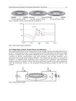
Active Suspension Systems
Consider the active suspension of a car seat given in (E. Reithmeier and G. Leitmann, 2003;
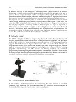
Assunção et al., 2007c) with other kind of control inputs, shown in Figure 8. The model
consists of a car mass M
c
and a driver-plus-seat mass m
s
. Vertical vibrations caused by a
street may be partially attenuated by shock absorbers (stiffness k
1
and damping b
1
).
Nonetheless, the driver may still be subjected to undesirable vibrations. These vibrations,
again, can be reduced by appropriately mounted car seat suspension elements (stiffness k
2

and damping b
2
). Damping of vibration of the masses M
c
and m
s

can be increased by
changing the control inputs u
1
(t) and u
2
(t). The dynamical system can be described by

11
22
12 2 12 2
33
44
2222
0010
00
() ()
0001
00
() ()
11
()
() ()
() ()
1
0
cccc cc
s
ssss
xt xt
xt xt

kk k bb b
ut
MMMM MM
xt xt
xt xt
kkbb
m
mmmm
⎡⎤
⎡⎤
⎢⎥
⎢⎥
⎡⎤ ⎡⎤
⎢⎥
⎢⎥
⎢⎥ ⎢⎥
⎢⎥
⎢⎥
−− −−
−
⎢⎥ ⎢⎥
=+
⎢⎥
⎢⎥
⎢⎥ ⎢⎥
⎢⎥
⎢⎥
⎢⎥ ⎢⎥
⎢⎥
⎢⎥

−−
⎣⎦ ⎣⎦
⎢⎥
⎢⎥
⎢⎥
⎢⎥
⎣⎦
⎣⎦




, (51)
Systems, Structure and Control

16

1
12
23
4
()
() ()
1000
() ()
0100
()
x
t
yt x t

yt xt
x
t
⎡
⎤
⎢
⎥
⎡⎤
⎡⎤
⎢
⎥
=
⎢⎥
⎢⎥
⎢
⎥
⎣⎦
⎣⎦
⎢
⎥
⎣
⎦
. (52)
The state vector is defined by
1212
()[()()()()]
T
x
t xtxtxtxt=


.
As in (E. Reithmeier and G. Leitmann, 2003), for feedback only the accelerations signals
1
()
x
t

and
2
()
x
t

are available (that are measured by accelerometer sensors). The velocities
1
()
x
t

and
2
()
x
t

are estimated from their measured time derivatives. Therefore the
accelerations and velocities signals are available (derivative of states), and so one can use the
proposed method to solve the problem.
Consider that the driver weight can assume values between 50kg and 100kg. Then the
system in Figure 8 has an uncertain constant parameter m

s
such that, 70kg ≤ m
s
≤ 120kg.
Additionally, suppose that can also happen a fail in the damper of the seat suspension (in
other words, the damper can break after some time). The fault can be described by a
polytopic uncertain system, where the system parameters without failure correspond to a
vertice of the polytopic, and with failures, the parameters are in another vertice. Then, one
can obtain the polytopic plant given in (25) and (26), composed by the polytopic sets due the
failures and the uncertain plant parameters.


Figure 8. Active suspension of a car seat
Control Designs for Linear Systems Using State-Derivative Feedback

17
The damper of the seat suspension b
2
can be considered as an uncertain parameter such that:
b
2
= 5 x 10
2
Ns/m while the damper is working and b
2
= 0 when the damper is broken.
Hence, and supposing M
c
= 1500kg (mass of the car), k
1

= 4 x 10
4
N/m (stiffness), k
2
= 5 x
10
3
N/m (stiffness) and b
1
= 4 x 10
3
Ns/m (damping), the plant (51) and (52) can be described
by equations (25), (26) and (45), and the matrices A
i
and B
j
, where r
a
= 4, r
b
, = 2, are given by:
12
0010 0010
0001 0001
,
30 3.33 3 0.33 30 3.33 3 0.33
71.43 71.43 7.143 7.143 41.67 41.67 4.167 4.167
AA
⎡⎤⎡ ⎤
⎢⎥⎢ ⎥

⎢⎥⎢ ⎥
==
⎢⎥⎢ ⎥
−− −−
⎢⎥⎢ ⎥
−− −−
⎣⎦⎣ ⎦
,
while the damper is working (in this case b
2
= 5 x 10
2
Ns/m, m
s
= 70kg in A
1
and m
s
= 120kg
in A
2
),
34
0010 0010
0001 0001
,
30 3.33 2.67 0 30 3.33 2.67 0
71.43 71.43 0 0 41.67 41.67 0 0
AA
⎡

⎤⎡ ⎤
⎢
⎥⎢ ⎥
⎢
⎥⎢ ⎥
==
⎢
⎥⎢ ⎥
−− −−
⎢
⎥⎢ ⎥
−−
⎣
⎦⎣ ⎦
,
when the damper is broken (in this case b
2
= 0, m
s
= 70kg in A
3
and m
s
= 120kg in A
4
) and
12
44 44
23
00 00

00 00
,
6.67 10 6.67 10 6.67 10 6.67 10
0 1.43 10 0 8.33 10
BB
−− −−
−−
⎡
⎤⎡ ⎤
⎢
⎥⎢ ⎥
⎢
⎥⎢ ⎥
==
⎢
⎥⎢ ⎥
×−× ×−×
⎢
⎥⎢ ⎥
⎢
⎥⎢ ⎥
××
⎣
⎦⎣ ⎦
,
because the input matrix
()B
β
depends only on the uncertain parameter m
s

(in this case m
s

= 70kg in B
1
and m
s
= 120kg in B
2
). Specifying an output peak bound
0
ξ
= 300, an initial
condition x(0) = [0.1 0.3 0 0]
T
and using the MATLAB (Gahinet et al, 1995) to solve the LMI
(32) and (33) from Theorem 2, with (47) and (48), the feasible solution was:
44 44
44 44
445 4
4445
2.400610 2.281210 4.109910 2.657810
2.2812 10 2.3265 10 2.1628 10 2.9019 10
4.1099 10 2.1628 10 5.29 10 8.3897 10
2.6578 10 2.9019 10 8.3897 10 1.8199 10
Q
⎡
⎤
××−×−×
⎢

⎥
××−×−×
⎢
⎥
=
⎢
⎥
−×−× × ×
⎢
⎥
⎢
⎥
−×−× × ×
⎣
⎦
,
6768
66 67
7.9749 10 3.0334 10 4.4436 10 6.5815 10
1.7401 10 2.2947 10 8.0344 10 1.616 10
Y
⎡
⎤
−×−×−× ×
=
⎢
⎥
××−×−×
⎢
⎥

⎣
⎦
.
From (34), we obtain the state-derivative feedback matrix below:
Systems, Structure and Control

18

33
. 10 923.6 442.06 4.3902 10
498.14 471.29 22.567 75.996
K
⎡
⎤
×− ×
=
⎢
⎥
−−−
⎢
⎥
⎣
⎦
2 894
. (53)
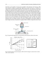
The locations in the s-plane of the eigenvalues
i
λ , for the eight vertices (A
i
, B

j
), i = 1, 2, 3, 4
and j = 1, 2, of the robust controlled system, are plotted in Figure 9. There exist four
eigenvalues for each vertice.
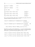
Consider that driver weight is 70kg, and so m
s
= 90kg. Using the designed controller (53)
and the initial condition x(0) defined above, the controlled system was simulated. The
transient response and the control inputs (30), of the controlled system, while the damper is
working are presented in Figures 10 and 11. Now suppose that happen a fail in the damper
of the seat suspension b
2
after 1s (in other words, b
2
= 5 x 10
2
Ns/m if t ≤ 1s and b
2
= 0 if t >
1s). Then, the transient response and the control inputs (30), of the controlled system, are
displayed in Figures 12 and 13. The required condition
0
() () 300max ytyt
′
<ξ = was
satisfied.


Figure 9. The eigenvalues in the eight vertices of the controlled uncertain system

Figure 10. Transient response of the system with the damper working
Control Designs for Linear Systems Using State-Derivative Feedback

19

Figure 11. Control inputs of the controlled system with the damper working

Figure 12. Transient response of the system with a fail in the damper b
2
after 1s

Figure 13. Control inputs of the controlled system with a fail in the damper b
2
after 1s
Systems, Structure and Control

20
Observe in Figures 10 and 12, that the happening of a fail in the damper b
2
does not change
the settling time of the controlled system, and had little influence in the control inputs.
Furthermore, as discussed before, considering m
s
= 90kg and the controller (53), the matrix
(())
I
BK+
β
has a full rank (det (())
I

BK+
β
= 0.85868 ≠ 0).
There exist problems where only the stability of the controlled system is insufficient to
obtain a suitable performance. Specifying a lower bound for the decay rate equal
γ
= 3, to
obtain a fast transient response, Theorem 3 is solved with (47) and (48) (
0
ξ
= 300). The
solution obtained with the software MATLAB was:
33 44
33 44
4455
4455
. 10 3.1064 10 2.6316 10 1.6730 10
. 0 10 3.6868 10 1.3671 10 1.8038 10
. 10 1.3671 10 5.3775 10 1.0319 10
1.6730 10 1.8038 10 1.0319 10 1.9587 10
Q
⎡
⎤
× ×−×−×
⎢
⎥
× ×−×−×
⎢
⎥
=

⎢
⎥
−×−× × ×
⎢
⎥
⎢
⎥
−×−× × ×
⎣
⎦
3 9195
31 64
26316
,
77 8 8
66 67
4.3933 10 2.8021 10 7.9356 10 1.6408 10
1.3888 10 1.8426 10 9.1885 10 1.69 10
Y
⎡
⎤
××−×−×
=
⎢
⎥
××−×−×
⎢
⎥
⎣
⎦

.
From (41), we obtain the state-derivative feedback matrix below:

33
621 3.8664 10 1.452 10 230.33
313.58 365.55 8.79 74.77
K
⎡
⎤
−×−×
=
⎢
⎥
−−−
⎢
⎥
⎣
⎦
(54)
The locations in the s-plane of the eigenvalues
i
λ , for the eight vertices (A
i
, B
j
), i = 1, 2, 3, 4
and j = 1, 2, of the robust controlled system, are plotted in Figure 14. There exist four
eigenvalues for each vertice.

Figure 14. The eigenvalues in the eight vertices of the controlled uncertain system
Control Designs for Linear Systems Using State-Derivative Feedback

21
From Figure 14, one has that all eigenvalues of the vertices have real part lower than
3−
γ
=− . Therefore, the controlled uncertain system has a decay rate greater or equal to
γ
.
Again, considering that m
s
= 90kg and using the designed controller (54) the matrix
(())
I
BK+
β
has a full rank (det (())
I
BK+
β
= 0.026272). For the initial condition x(0)
defined above, the controlled system was simulated. The transient response and the control
inputs (30) of the controlled system are presented in Figures 15, 16, 17 and 18, respectively.

Figure 15. Transient response of the system with the damper working
Observe that, the settling time in Figures 15 and 17 are smaller than the settling time in
Figures 10 and 12, where only stability was required and also,
() ()max ytyt
′

is equal to
0.31623 <
0
300
ξ
= . Then, the specifications were satisfied by the designed controller (54).
Moreover, the happening of a fail in the damper b
2
does not significantly change the settling
time (Figures 15 and 17) of the controlled system. In spite of the change in the control inputs
from Figures 16 and 18, the fail in the damper does not changed the maximum absolute
value of the control signal (u(t) = 1.1161 x 10
5
N).

Figure 16. Control inputs of the controlled system with the damper working
Systems, Structure and Control

22

Figure 17. Transient response of the system with a fail in the damper b
2
after 0.3s


Figure 18. Control inputs of the controlled system with a fail in the damper b
2
after 0.3s
Note that some absolute values of the entries of (53) and (54) are great values and it could be
a trouble for the practical implementation of the controller. For the reduction of this problem

in the implementation of the controller, the specification of bounds on the state-derivative
feedback matrix K can be done using the optimization procedure stated in Theorem 4, with
0
μ
= 0.1. The optimal values, obtained with the software MATLAB, for Theorem 4
considering: (33) for stability, or (40) for stability with bound on the decay rate (
γ
= 3), and
(47) and (48) (
0
ξ
= 300) are displayed in Table 1. Considering that m
s
= 90kg and the initial
condition x(0) defined above, the transient response and the control inputs obtained by
Theorem 4 considering (33) or (40), are displayed in Figures 19, 20, 21 and 22 respectively.
Control Designs for Linear Systems Using State-Derivative Feedback

23
Theorem 4 with (33) Theorem 4 with (40)
Q =
⎡⎤
⎢⎥
⎢⎥
⎢⎥
⎣⎦
1.2265 1.5357 -1.667 -5.8859
1.5357 2.5422 0.6289 -5.1654
-1.667 0.6289 27.177 30.007
-5.8859 -5.1654 30.007 67.502

0.16831 0.088439 0.52166 0.25122
.088439 0.56992 0.07813 2.3703
0.52166 0.07813 5.1595 2.9849
0.25122 2.3703 2.9849 43.238
0
Q
−−
−−
−− −
−−
=
⎡
⎤
⎢
⎥
⎢
⎥
⎢
⎥
⎣
⎦

Y =
⎡⎤
⎢⎥
⎣⎦
17.423 19.928 -13.793 12.407
-25.896 20.088 -2.8711 0.69624
Y =

⎡
⎤
⎢
⎥
⎣
⎦
3
918.06 749.73 -3.3745×10 204.86
3
30.057 468.97 -102.46 -3.5475×10

K =
⎡⎤
⎢⎥
⎣⎦
39.536 -6.5518 -2.7229 4.3402
-276.41 173.56 -17.953 -2.829
K =
⎡
⎤
⎢
⎥
⎣
⎦
3
4.7321×10 859.72 -121.49 70.976
-559.07 664.62 -98.521 -55.661

Table 1. The solutions with Theorem 4

Figure 19. Transient response of the system with a fail in the damper b
2
after 1s, obtained
with Theorem 4 and (33)
Systems, Structure and Control

24

Figure 20. Control inputs of the controlled system with a fail in the damper b
2
after 1s

Figure 21. Transient response of the system with a fail in the damper b
2
after 0.3s, obtained
with Theorem 4 and (40)

Figure 22. Control inputs of the controlled system with a fail in the damper b
2
after 0.3s
Control Designs for Linear Systems Using State-Derivative Feedback

25
The matrix norm of the controller (53) obtained with Theorem 2 is equal to
K
= 5.3628xl0
3

and the maximum absolute value of the control signal is u(t) = 6.0356 x 10
4
N, while that the
matrix norm of the same controller obtained with Theorem 4 considering (33) is equal to
K
= 328.96 and the maximum absolute value of the control signal is u(t) = 68.111N.
Then, Theorem 4 was able to stabilize the controlled system with a smaller state-derivative
feedback matrix gain. The similar form, the maximum absolute value of the control signal
u(t) from (54), obtained with Theorem 3 is u(t) = 1.1161 x 10
5
N, and of the same controller
obtained with Theorem 4 considering (40) is u(t) = 2.0362 x 10
3
N. This example shows that
the proposed methods are simple to use and it is easy to specify the constraints in the
design.
4. Conclusions
In this chapter two new control designs using state-derivative feedback for linear systems
were presented. Firstly, considering linear descriptor plants, a simple method for designing
a state-derivative feedback gain (K
d
) using methods for state feedback control design was
proposed. The descriptor linear systems must be time-invariant, Single-Input (SI) or
Multiple-Input (MI) system. The procedure allows that the designers use the well-known
state feedback design methods to directly design state-derivative feedback control systems.
This method extends the results described in (Cardim et al, 2007) and (Abdelaziz & Valášek,
2004) to a more general class of control systems, where the plant can be a descriptor system.
As the first design can not be directly applied for uncertain systems, then a design
considering sufficient stability conditions based on LMI for state-derivative feedback, that
provide an extension of the methods presented in (Assunção et al., 2007c) were presented.

The designers can include in the LMI-based control design, the specification of the decay
rate and bounds on output peak and on state-derivative feedback gains. The plant can be
subject to structural failures. So, in this case, one has a fault-tolerant design. Furthermore,
the new design methods allow a broader class of plants and performance specifications,
than the related results available in the literature, for instance in (E. Reithmeier and G.
Leitmann, 2003; Abdelaziz & Valášek, 2004; Duan et al., 2005; Assunção et al., 2007c; Cardim
et al., 2007). The presented method offers LMI-based designs for state-derivative feedback
that, when feasible, can be efficiently solved by convex programming techniques. In Sections
2.3 and 3.5, the validity and simplicity of the new control designs can be observed with
some numerical examples.
5. Acknowledgments
The authors acknowledge the financial support by FAPESP, CAPES and CNPq, from Brazil.
6. References
A. Bunse-Gerstner, R. Byers, V. M. & Nichols, N. (1999), Feedback design for regularizing
descriptor systems, in Linear Algebra and its Applications, pp. 119-151.
Abdelaziz, T. H. S. & Valášek, M. (2005), Direct Algorithm for Pole Placement by State-
Derivative Feedback for Multi-Input Linear Systems - Nonsingular Case,
Kybernetika 41(5), 637-660.
Systems, Structure and Control

26
Abdelaziz, T. H. S. & Valášek, M. (2004), Pole-placement for SISO Linear Systems by State-
Derivative Feedback, IEE Proceedings-Control Theory Applications 151(4), 377-385.
Assunção, E., Andrea, C. Q. & Teixeira, M. C. M. (2007a),
2
and
∞
, -optimal control for
the tracking problem with zero variation, IET Control Theory Applications 1(3), 682-
688.

Assunção, E., Marchesi, H. E, Teixeira, M. C. M. & Peres, P. L. D. (2007b), Global
Optimization for the H
∞
-Norm Model Reduction Problem, International Journal of
Systems Science 38(2), 125-138.
Assunção, E. & Peres, P. L. D. (1999), A global optimization approach for the
2
-norm
model reduction problem, in Proceedings of the 38th IEEE Conference on Decision
and Control, Phoenix, AZ, USA, pp. 1857-1862.
Assunção, E., Teixeira, M. C. M., Faria, F. A., da Silva, N. A. P. & Cardim, R. (2007c),
Robust State-Derivative Feedback LMI-Based Designs for Multivariable Linear
Systems, International Journal of Control 80(8), 1260-1270.
Boyd, S., El Ghaoui, L., Feron, E. & Balakrishnan, V. (1994), Linear Matrix Inequalities in
Systems and Control Theory, 2nd edn, SLAM Studies in Applied Mathematics,
USA. boyd/lmibook/lmibook.pdf.
Bunse-Gerstner, A., Nichols, N. & Mehrmann, V. (1992), Regularization of Descriptor
Systems by Derivative and Proportional State Feedback, in SIAM J. Matrix Anal
Appl., pp. 46-67.
Cardim, R., Teixeira, M. C. M., Assunção, E. & Covacic, M. R. (2007), Design of State-
Derivative Feedback Controllers Using a State Feedback Control Design, in 3rd
IFAC Symposium on System, Structure and Control, Vol. 1, Iguassu Falls, PR, Brazil,
pp. Article 135-6 pages.
Chen, C. T. (1999), Linear System Theory and Design, 2nd edn, Oxford University Press,
New York.
D. Ye & G. H. Yang (2006), Adaptive fault-tolerant tracking control against actuator faults
with application to flight control, Control Systems Technology, IEEE Transactions on
14(6), 1088-1096.
de Oliveira, M. C., Farias, D. P. & Geromel, J. C. (1997), LMISol, User's guide, UNICAMP,

Campinas-SP, Brazil,
Duan, G. R., Irwin, G. W. & Liu, G. P. (1999), Robust Stabilization of Descriptor Linear
Systems via Proportional-plus-derivative State Feedback, in Proceedings of the
1999 American Control Conference, San Diego, CA, USA, pp. 1304-1308.
Duan, G. R. & Zhang, X. (2003), Regularizability of Linear Descriptor Systems via Output
plus Partial State Derivative Feedback, Asian Journal of Control 5(3), 334-340.
Duan, Y. E, Ni, Y Q. & Ko, J. M. (2005), State-Derivative feedback control of cable
vibration using semiactive magnetorheological dampers, Computer-Aided Civil and
Infrastructure Engineering 20(6), 431-449.
E. Reithmeier and G. Leitmann (2003), Robust vibration control of dynamical systems
based on the derivative of the state, Archive of Applied Mechanics 72(11-12), 856-
864.
El Ghaoui & Niculescu, S. (2000), Advances in Linear Matrix Inequalities Methods in Control,
SIAM Advances in Design and Control, USA.
Gahinet, P., Nemirovski, A., Laub, A. J. & Chilali, M. (1995), LMI control toolbox - For use
with Matlab, The Math Works Inc.
Control Designs for Linear Systems Using State-Derivative Feedback

27
Isermann, R. (1997), Supervision, fault-detection and fault-diagnosis methods - an
introduction, Control Engineering Practice 5(5), 639-652.
Isermann, R. (2006), Fault-Diagnosis systems: An introduction from fault detection to fault
tolerance, Springer, Berlin.
Isermann, R. & Ballé, P. (1997), Trends in the application of model-based fault detection
and diagnosis of technical processes, Control Engineering Practice 5(5), 709-719.
Kwak, S. K., Washington, G. & Yedavalli, R. K. (2002), Acceleration-Based vibration
control of distributed parameter systems using the "reciprocal state-space
framework", Journal of Sound and Vibration 251(3), 543-557.
Liu, J., Wang, J. L. & Yang, G. H. (2005), An LM1 approach to minimum sensitivity
analysis with application to fault detection, Automatica 41(11), 1995-2004.

Nesterov, Y. & Nemirovsky, A. (1994), Interior-Point Polynomial Algorithms in Convex
Programming, SLAM Studies in Applied Mathematics, USA.
Nichols, N., Bunse-Gerstner, A. & Mehrmann, V. (1992), Regularization of descriptor
systems by derivative and proportional state feedback, in SIAM J. Matrix Anal.
Appl., pp. 46-67.
Ogata, K. (2002), Modern Control Engineering, 4th edn, Prentice-Hall, New Jersey.
Palhares, R. M., Hell, M. B., Duraes, L. M., Ribeiro Neto, J. L., Teixeira, M. C. M. &
Assunção, E. (2003), Robust H
∞
Filtering for a Class of State-delayed Nonlinear
Systems in an LMI Setting, International Journal Of Computer Research 12(1), 115-
122.
S. S. Yang & J. Chen (2006), Sensor faults compensation for MLMO fault-tolerant control
systems, Transactions of the Institute of Measurement and Control 28(2), 187-205.
S. Xu & J. Lam (2004), Robust Stability and Stabilization of Discrete Singular Systems: An
Equivalent Characterization, IEEE Transactions on Automatic Control 49(4), 568-
574.
Sturm, J. (1999), Using SeDuMi 1.02, a MATLAB toolbox for optimization over symmetric
cones, Optimization Methods and Software 11-12, 625-653.

Teixeira, M. C. M., Assunção, E. & Avellar, R. G. (2003), On relaxed LMI-based designs for
fuzzy regulators and fuzzy observers, IEEE Transactions on Fuzzy Systems 11(5),
613-623.
Teixeira, M. C. M., Assunção, E. & Palhares, R. M. (2005), Discussion on: H
∞
Output
Feedback Control Design for Uncertain Fuzzy Systems with Multiple Time
Scales: An LMI Approach, European Journal of Control 11(2), 167-169.
Teixeira, M. C. M, Assunção, E. & Pietrobom, H. C. (2001), On Relaxed LMI-Based Design
Fuzzy, in Proceedings of the 6th European Control Conference, Porto, Portugal, pp.

120-125.
Teixeira, M. C. M., Covacic, M., Assunção, E. & Lordelo, A. D. (2002), Design of SPR
Systems and Output Variable Structure Controllers Based on LMI, in 7th IEEE
International Workshop on Variable Structure Systems, Vol. 1, Sarajevo, Bosnia, pp.
133-144.
Teixeira, M. C. M., Covacic, M. R. & Assunção, E. (2006), Design of SPR Systems with
Dynamic Compensators and Output Variable Structure Control, in International
Workshop on Variable Structure Systems, Vol. 1, Alghero-Italy, pp. 328-333.
Systems, Structure and Control

28
Valášek, M. & Olgac, N. (1995a), An Efficient Pole-Placement Technique for Linear Time-
Variant SISO System, 1EE Proceedings-Control Theory and Applications 142(5), 451-
458.
Valášek, M. & Olgac, N. (1995b), Efficient Eigenvalue Assignments for General Linear
MIMO Systems, Automatica 31(11), 1605-1617.
Zhong, M., Ding, S. X., Lam, J. & Wang, H. (2003),'An LMI approach to design robust fault
detection filter for uncertain LTI systems, Automatica 39(3), 543-550.
2
Asymptotic Stability Analysis of Linear Time-
Delay Systems: Delay Dependent Approach
Dragutin Lj. Debeljkovic
1
and Sreten B. Stojanovic
2

1
University of Belgrade, Faculty of Mechanical Engineering
2
University of Nis, Faculty of Technology

Serbia
1. Introduction
The problem of investigation of time delay systems has been exploited over many years.
Time delay is very often encountered in various technical systems, such as electric,
pneumatic and hydraulic networks, chemical processes, long transmission lines, etc. The
existence of pure time lag, regardless if it is present in the control or/and the state, may
cause undesirable system transient response, or even instability.
During the last three decades, the problem of stability analysis of time delay systems has
received considerable attention and many papers dealing with this problem have appeared
(Hale & Lunel, 1993). In the literature, various stability analysis techniques have been utilized
to derive stability criteria for asymptotic stability of the time delay systems by many
researchers (Yan, 2001; Su, 1994; Wu & Muzukami, 1995; Xu, 1994; Oucheriah, 1995; Kim, 2001).
The developed stability criteria are classified often into two categories according to their
dependence on the size of the delay: delay-dependent and delay-independent stability
criteria (Hale, 1997; Li & de Souza, 1997; Xu et al., 2001). It has been shown that delay-
dependent stability conditions that take into account the size of delays, are generally less
conservative than delay-independent ones which do not include any information on the size
of delays.
Further, the delay-dependent stability conditions can be classified into two classes:
frequency-domain (which are suitable for systems with a small number of heterogeneous
delays) and time-domain approaches (for systems with a many heterogeneous delays).
In the first approach, we can include the two or several variable polynomials (Kamen 1982;
Hertz et al. 1984; Hale et al. 1985) or the small gain theorem based approach (Chen &
Latchman 1994).
In the second approach, we have the comparison principle based techniques
(Lakshmikantam & Leela 1969) for functional differential equations (Niculescu et al. 1995a;
Goubet-Bartholomeus et al. 1997; Richard et al. 1997) and respectively the Lyapunov
stability approach with the Krasovskii and Razumikhin based methods (Hale & Lunel 1993;
Kolmanovskii & Nosov 1986). The stability problem is thus reduced to one of finding
solutions to Lyapunov (Su 1994) or Riccati equations (Niculescu et al., 1994), solving linear

matrix inequalities (LMIs) (Boyd et al. 1994; Li & de Souza, 1995; Niculescu et al., 1995b; Gu
1997) or analyzing eigenvalue distribution of appropriate finite-dimensional matrices (Su
Systems, Structure and Control

30
1995) or matrix pencils (Chen et al., 1994). For further remarks on the methods see also the
guided tours proposed by (Niculescu et al., 1997a; Niculescu et al., 1997b; Kharitonov, 1998;
Richard, 1998; Niculescu & Richard, 2002; Richard, 2003).
It is well-known (Kolmanovskii & Richard, 1999) that the choice of an appropriate
Lyapunov–Krasovskii functional is crucial for deriving stability conditions. The general
form of this functional leads to a complicated system of partial differential equations
(Malek-Zavareiand & Jamshidi, 1987). Special forms of Lyapunov–Krasovskii functionals
lead to simpler delay-independent (Boyd et al., 1994; Verriest & Niculescu, 1998;
Kolmanovskii & Richard, 1999) and (less conservative) delay-dependent conditions (Li & de
Souza, 1997; Kolmanovskii et al., 1999; Kolmanovskii & Richard, 1999; Park, 1999; Lien et al.,
2000; Niculescu, 2001). Note that the latter simpler conditions are appropriate in the case of
unknown delay, either unbounded (delay-independent conditions) or bounded by a known
upper bound (delay-dependent conditions).
In the delay-dependent stability case, special attention has been focused on the first delay
interval guaranteeing the stability property, under some appropriate assumptions on the
system free of delay. Thus, algorithms for computing optimal (or suboptimal) bounds on the
delay size are proposed in (Chiasson, 1988; Chen et al., 1994) (frequency-based approach), in
(Fu et al., 1997) (integral quadratic constraints interpretations), in (Li & de Souza, 1995;
Niculescu et al., 1995b; Su, 1994) (Lyapunov-Razumikhin function approach) or in (Gu,
1997) (discretization schemes for some Lyapunov- Krasovskii functionals). For computing
general delay intervals, see, for instance, the frequency based approaches proposed in
(Chen, 1995).
In the past few years, there have been various approaches to reduce the conservatism of
delay-dependent conditions by using new bounding for cross terms or choosing new
Lyapunov–Krasovskii functional and model transformation. The delay-dependent stability

criterion of (Park et al., 1998; Park, 1999) is based on a so-called Park’s inequality for
bounding cross terms. However, major drawback in using the bounding of (Park et al., 1998)
and (Park, 1999) is that some matrix variables should be limited to a certain structure to
obtain controller synthesis conditions in terms of LMIs. This limitation introduces some
conservatism. In (Moon et al., 2001) a new inequality, which is more general than the Park’s
inequality, was introduced for bounding cross terms and controller synthesis conditions
were presented in terms of nonlinear matrix inequalities in order to reduce the
conservatism. It has been shown that the bounding technique in (Moon et al., 2001) is less
conservative than earlier ones. An iterative algorithm was developed to solve the nonlinear
matrix inequalities (Moon et al., 2001).
Further, in order to reduce the conservatism of these stability conditions, various model
transformations have been proposed. However, the model transformation may introduce
additional dynamics. In (Fridman & Shaked, 2003) the sources for the conservatism of the
delay-dependent methods under four model transformations, which transform a system
with discrete delays into one with distributed delays are analyzed. It has been demonstrated
that descriptor transformation, that has been proposed in (Fridman & Shaked, 2002a), leads
to a system which is equivalent to the original one, does not depend on additional
assumptions for stability of the transformed system and requires bounding of fewer cross-
terms. In order to reduce the conservatism, (Han, 2005a; Han, 2005b) proposed some new
methods to avoid using model transformation and bounding technique for cross terms.
Asymptotic Stability Analysis of Linear Time-Delay Systems: Delay Dependent Approach

31
In (Fridman & Shaked, 2002b) both the descriptor system approach and the bounding
technique using by (Moon et al., 2001) are utilized and the delay-dependent stability results
are performed. The derived stability criteria have been demonstrated to be less conservative
than existing ones in the literature.
Delay-dependent stability conditions in terms of linear matrix inequalities (LMIs) have been
obtained for retarded and neutral type systems. These conditions are based on four main
model transformations of the original system and application mentioned inequalities.

The majority of stability conditions in the literature available, of both continual and discrete
time delay systems, are sufficient conditions. Only a small number of works provide both
necessary and sufficient conditions, (Lee & Diant, 1981; Xu et al., 2001; Boutayeb &
Darouach, 2001), which are in their nature mainly dependent of time delay. These
conditions do not possess conservatism but often require more complex numerical
computations. In our paper we represent some necessary and sufficient stability conditions.
Less attention has been drawn to the corresponding results for discrete-time delay systems
(Verriest & Ivanov, 1995; Kapila & Haddad, 1998; Song et al., 1999; Mahmoud, 2000; Lee &
Kwon, 2002; Fridman & Shaked, 2005; Gao et al., 2004; Shi et al., 2000). This is mainly due to
the fact that such systems can be transformed into augmented high dimensional systems
(equivalent systems) without delay (Malek-Zavarei & Jamshidi, 1987; Gorecki et al., 1989).
This augmentation of the systems is, however, inappropriate for systems with unknown
delays or systems with time varying delays. Moreover, for systems with large known delay
amounts, this augmentation leads to large-dimensional systems. Therefore, in these cases
the stability analysis of discrete time delay systems can not be to reduce on stability of
discrete systems without delay.
In our paper we present delay-dependent stability criteria for particular classes of time
delay systems: continuous and discrete time delay systems and continuous and discrete
time delay large-scale systems. Thereat, these stability criteria are express in form necessary
and sufficient conditions.
The organization of this chapter is as follows. In section 2 we present necessary and
sufficient conditions for delay-dependent asymptotic stability of particular class of
continuous and discrete time delay systems. Moreover, we show that in the paper of (Lee &
Diant, 1981) there are some mistakes in formulation of particular theorems. We correct these
errors and extend derived results on discrete time delay systems. Further extensions of these
results to the class of continuous and discrete large scale time delay systems are presented in
the section 3. All theoretical results are supported by suitable chosen numerical examples.
And section 4 discuss and summarizes contributions.
2. Time delay systems
Throughout this chapter we use the following notation.  and  denote real (complex)

vector space or the set of real (complex) numbers,
T
+
denotes the set of all non-negative
integers,
*
λ means conjugate of λ∈ and F
∗
conjugate transpose of matrix
nn
F
×
∈ .
Re(s) is the real part of s∈ . The superscript T denotes transposition. For real matrix
F the
notation F 0> means that the matrix F is positive definite.
()
i
Fλ
is the eigenvalue of
matrix
F . Spectrum of matrix F is denoted with
()
Fσ and spectral radius with
()
Fρ .
Systems, Structure and Control

32
2.1 Continuous time delay systems

For the sake of completeness, we present the following result (Lee & Diant, 1981). Considers
class of continuous time-delay systems described by

() () ( ) () ()
01
xt A xt A xt , xt t, t 0=+−τ=−τ≤<

ϕ
(1)
Theorem 2.1.1 (Lee & Diant, 1981) Let the system be described by (1). If for any given matrix
*
QQ 0=>
there exist matrix
*
PP 0=>, such that

()
()
()
()
T
00
PA T0 A T0 P Q+++ =− (2)
where
()
Tt
is continuous and differentiable matrix function which satisfies

()
()

()
() ()
01
AT0Tt,0t,T A
Tt
0,t
⎧
+≤≤ττ=
⎪
=
⎨
>τ
⎪
⎩

(3)
then the system (1) is asymptotically stable.
In paper (Lee & Diant, 1981) it is emphasized that the key to the success in the construction
of a Lyapunov function corresponding to the system (1) is the existence of at least one
solution
()
T t of (3) with boundary condition
()
1
TAτ=
. In other words, it is required that
the nonlinear algebraic matrix equation

()
()

()
0
AT0
1
eT0A
+τ
= (4)
has at least one solution for
()
T 0 . It is asserted, there, that asymptotic stability of the system
(
Theorem 2.1.1) can be determined based on the knowledge of only one or any, solution of the
particular nonlinear matrix equation.
We now demonstrate that
Theorem 2.1.1 should be improved since it does not take into
account all possible solutions for (4). The counterexample, based on our approach and
supported by the Lambert function application, is given in (Stojanovic & Debeljkovic, 2006).
Conclusion 2.1.1 (Stojanovic & Debeljkovic, 2006) If we introduce a new matrix,

()
1
RA T0+ (5)
then condition (2) reads

*
PR R P Q+=− (6)
which presents a well-known Lyapunov’s equation for the system without time delay.
This condition will be fulfilled if and only if R is a stable matrix i.e. if

()

Re R 0
i
λ< (7)
holds.
Let
T
Ω and
R
Ω denote sets of all solutions of eq. (4) per T(0) and (6) per R, respectively.