Báo cáo hóa học: " Research Article Bargaining and the MISO Interference Channel" ppt

Hindawi Publishing Corporation
EURASIP Journal on Advances in Signal Processing
Volume 2009, Article ID 368547, 13 pages
doi:10.1155/2009/368547
Research Article
Bargaining and the MISO Interference Channel
Matthew Nokleby
1
and A. Lee Swindlehurst
2
1
Department of Electrical and Computer Engineering, Rice University, Houston, TX 77005, USA
2
Department of Electrical Engineering and Computer Science, University of California at Irvine, Irvine,
CA 92697, USA
Correspondence should be addressed to Matthew Nokleby,
Received 31 October 2008; Revised 27 February 2009; Accepted 8 April 2009
Recommended by Eduard A. Jorswieck
We examine the MISO interference channel under cooperative bargaining theory. Bargaining approaches such as the Nash and
Kalai-Smorodinsky solutions have previously been used in wireless networks to strike a balance between max-sum efficiency
and max-min equity in users’ rates. However, cooperative bargaining for the MISO interference channel has only been studied
extensively for the two-user case. We present an algorithm that finds the optimal Kalai-Smorodinsky beamformers for an arbitrary
number of users. We also consider joint scheduling and beamformer selection, using gradient ascent to find a stationary point of
the Kalai-Smorodinsky objective function. When interference is strong, the flexibility allowed by scheduling compensates for the
performance loss due to local optimization. Finally, we explore the benefits of power control, showing that power control provides
nontrivial throughput gains when the number of transmitter/receiver pairs is greater than the number of transmit antennas.
Copyright © 2009 M. Nokleby and A. L. Swindlehurst. This is an open access article distributed under the Creative Commons
Attribution License, which permits unrestricted use, distribution, and reproduction in any medium, provided the original work is
properly cited.
1. Introduction
After more than a decade of intense research, multiantenna

communications systems are sufficiently well understood
that they now appear in current and emerging wireless
standards [1, 2]. Because they offer increased spatial flexi-
bility, multiple-antenna systems are particularly well suited
to multiuser communications. Generally speaking, multiuser
communication presents a complicated problem partially
because performance criteria are difficult to characterize.
There is no, for example, single data rate or bit-error proba-
bility to optimize. Instead, we can only maximize composite
performance measures such as the network sum rate, max-
min fairness, or quality-of-service requirements. Ultimately,
the choice of objective function is often somewhat arbitrary.
To meet this challenge, researchers have begun to apply
game theory [3], a mathematical idealization of human
decision-making, to problems in multiuser communica-
tions. Game theory provides a systematic framework for
the study of decision makers with potentially conflicting
interests, as well as solutions for such conflicts. Accord-
ingly, a game-theoretic analysis can provide a tractable,
structured approach to resource allocation. Researchers have
successfully employed game-theoretic ideas to design “fair”
medium-access protocols, develop decentralized network
algorithms, and otherwise solve resource-allocation prob-
lems in communications networks [4–10].
In this paper, we study the multiple-input single-output
(MISO) interference channel. In the MISO interference
channel, several communication links, each involving a
multiantenna transmitter and a single-antenna receiver, are
simultaneously active. This scenario models, for example,
intercell interference in cellular systems or MIMO networks

where receivers employ fixed beamformers. Multilink MISO
systems have been studied in a number of previous works.
For example, in [11, 12], the MISO broadcast channel is
studied from the intercell interference point of view, with
emphasis on maximizing the network sum rate. The same
scenario is addressed in [13], but max-min fairness is used
to improve the performance of weaker network links. Game-
theoretic solutions for the MISO interference channel based
on bargaining have been considered in [14, 15], but only for
the two-user case.
Our particular focus is to maximize network perfor-
mance according to the Kalai-Smorodinsky solution [16],
2 EURASIP Journal on Advances in Signal Processing
a cooperative bargaining approach closely related to the
well-known Nash bargaining solution [17]. For our prob-
lem, the fundamental idea of the Kalai-Smorodinsky (K-
S) approach is to maximize users’ rates while ensuring
that users experience the same fraction of the rate they
would achieve without interference. In practice, the K-S
solution defines a compromise between efficiency (defined
herein in terms of maximizing the sum rate) and equity
(maximizing the minimum rate). Our primary contribution
is an algorithm that efficiently finds the K-S solution for
an arbitrary number of users, rather than just the two-
user case. We transform the rate-maximization problem to a
series of convex programming problems, allowing us to find
the beamformers that achieve the rates defined by the K-S
solution.
A drawback of the K-S solution is that when interference
becomes strong for a single user, all users’ bargained

rates tend toward zero. To avoid this, we also study joint
scheduling and beamformer selection under K-S bargaining,
which introduces a temporal degree of freedom for avoiding
interference. Scheduling also convexifies the feasible rate
region, which is an important consideration in cooperative
bargaining. However, the need to jointly address scheduling
and beamformer selection complicates the optimization,
preventing us from easily finding the K-S solution. We there-
fore devise a gradient-based algorithm to find a stationary
point of the K-S objective function. While we sacrifice global
optimality to include scheduling, the performance advantage
of employing time-division multiplexing significantly out-
weighs the potential loss of optimality when the interference
is strong.
The paper is organized as follows: in Section 2 we present
the system model, discussing the achievable rates and a
few simple beamforming strategies. In Section 3 we briefly
introduce the Kalai-Smorodinsky solution. In Section 4 we
present algorithms for selecting beamformers and (where
applicable) transmission schedules that achieve the Kalai-
Smorodinsky solution. In Section 5 we examine the fairness
and efficiency of our proposed algorithms and discuss the
effects of power control. Finally, we give our conclusions in
Section 6.
2. System Model
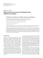
2.1. Signal Model. The K-user MISO interference channel, as
depicted in Figure 1, is composed of KN-antenna transmit-
ters, each of which intends to communicate with a unique
single-antenna receiver. We assume a narrowband channel
model where the ith transmitter sends a complex baseband

vector x
i
. The received signal y
i
contains the intended signal,
cochannel interference from the other K
−1 transmitters, and
additive Gaussian noise:
y
i
= h
H
i,i
x
i
+
K

j=1
j
/
=i
h
H
i,j
x
j
+ n
i
,(1)

where h
i,j
is the vector of complex channel gains between
the antennas of the jth transmitter and the ith receiver, and
x
1
h
11
h
12
y
1
x
2
h
22
h
21
y
2
Figure 1: Two-user MISO interference channel.
(·)
H
denotes the Hermitian transpose. We normalize the
channel gains such that—without loss of generality—n
i
has
unit variance. Particularly, we assume channels of the form
h
i,j

=
√
ρ
i,j

h
i,j
, where the elements of

h
i,j
are zero-mean,
unit-variance complex random variables, and ρ
i,j
represents
the expected channel gain between the jth transmitter and
the ith receiver.
2.2. Achievable Rates. To define the set of achievable rates
under our assumptions, we view each transmitted signal
x
i
as a zero-mean random vector characterized by the
covariance matrix P
i
= E{x
i
x
H
i
},whereE{·} denotes

statistical expectation. In principle, P
i
can be any positive
semidefinite matrix, although we focus on the rank-one case
due to the MISO setting considered here. Specifically, we
assume that x
i
is of the form x
i
= w
i
s
i
,wherew
i
is the
(fixed) transmit beamformer for user i,ands
i
is a zero-mean,
unit-variance Gaussian symbol. Thus, P
i
= w
i
w
H
i
, and the
spatial characteristics of the transmitted signal are entirely
characterized by the beamforming vector w
i

.
Each transmitter has limited peak power output, which
we model by constraining the norm of each beamformer:
w
i

2
≤ 1, where ·
2
denotes the 
2
norm. Let W
1
denote
the set of feasible beamformers:
W
1
=

w ∈ C
N
: w
2
≤ 1

. (2)
Here we have defined a general model where transmitters
choose both the magnitude of the beamformer, which
represents the transmit power, as well as its direction. When
the beamformers are unit-norm, the channel parameter ρ

i,j
represents the received signal-to-noise ratio (SNR) between
the jth transmitter and the ith receiver. We may wonder,
given the spatial freedom offered by the multiple antennas,
if such power control is necessary. For example, in [18]itis
shown that, when K
≤ N, only beamformers with w
i

2
= 1
are necessary, obviating the need for power control. However,
this result does not generalize, and in Section 5 we explore
the benefit of power control in a system with an arbitrary
number of users.
In determining achievable rates, we assume that trans-
mitters and receivers have full channel state information and
that the receivers employ single-user detection, meaning that
cochannel interference is treated as noise when decoding the
incoming signal. Under these assumptions, the rate across
EURASIP Journal on Advances in Signal Processing 3
the ith link is bounded by the mutual information between
x
i
and y
i
, which, in terms of the beamformers, is
I

x

i
; y
i

=
log
2
⎛
⎜
⎝
1+



h
H
i,i
w
i



2
1+

j
/
=i




h
H
i,j
w
j



2
⎞
⎟
⎠
. (3)
For notational convenience we will occasionally group
the beamformers into a single N
× K matrix W =
[w
1
w
2
··· w
K
]. Then, we can denote the mutual infor-
mation across the ith link as a function of the beamformers:
I
i
(W). The set of achievable rates is bounded by the mutual
information possible under all feasible beamformers:
R

=

r ∈ R
K
+
: r
i
≤ I
i
(
W
)
, W
∈ W
K
1

. (4)
The feasible set R has an important property which we will
exploit throughout the paper: it is comprehensive with respect
to the zero vector. A set S
⊂ R
K
is comprehensive with
respect to 0 provided that for every r
∈ S,0 s  r
implies s
∈ S,where and  represent element-wise vector
inequalities. In our case, the rate region R is comprehensive
because any user can—without altering its beamformer—

freely lower its rate without impacting other users’ rates.
2.3. Scheduling. In general, R is not convex, suggesting
that we may achieve higher rates—especially in cases of
strong interference—via time-sharing. (Alternatively, the
rate region may be convexified by other equivalent means
such as frequency-sharing or randomized beamformer selec-
tion). To do so, we divide each transmission into K time
blocks, during each of which the transmitters may use a
different beamformer. The mutual information during block
t is
I

x
i
(
t
)
; y
i
(
t
)

= log
2
⎛
⎜
⎝
1+




h
H
i,i
w
i
(t)



2
1+

j
/
=i



h
H
i,j
w
j
(t)



2

⎞
⎟
⎠
. (5)
We use I
i
(W(t)) to represent the mutual information during
the tth block.
The relative duration of each block is defined by the
scheduling vector a
=
[
a
1
··· a
K
]
, which obeys the constraints
a
 0and

K
t
=1
a
t
= 1. The scheduling weights in a define
a convex combination of the rates achieved during each
time block. With scheduling, the average achievable rate over
the ith link is bounded by the average mutual information


t
a
t
I(x
i
(t); y(t)). The set of feasible scheduling vectors is
A
=
⎧
⎨
⎩
a ∈ R
K
+
:
K

t=1
a
t
= 1
⎫
⎬
⎭
. (6)
Since time-sharing allows us to take convex combinations
of rate vectors, the set of achievable rates under scheduling,
denoted by
R, is the convex hull of R:

R =
⎧
⎨
⎩
r ∈ R
K
+
: r
i
≤
K

t=1
a
t
I
i
(
W
(
t
))
, a
∈ A, W
(
t
)
∈ W
K
1

, ∀t
⎫
⎬
⎭
.
(7)
To see that K time blocks are sufficient to achieve the convex
hull, note that the convex hull of R can be defined as the
intersection of all closed half-planes in
R
K
that contain R.
So, any boundary point on the convex hull of R must lie
on a convex subset of a bounding hyperplane in
R
K
defined
by at most K linearly independent boundary points of R.
Thus any point on the boundary of the convex hull can be
achieved by taking convex combinations of at most K points
in R. But, since R is comprehensive, we can reach any point
in the convex hull by choosing the nearest boundary point
and appropriately lowering the rates of the associated K
points. To see that K points are required in general, consider
an extreme case where ρ
i,j
=∞for i
/
= j, so only a single
transmitter can achieve a nonzero rate at a time. To realize

the boundary of the convex hull of R, each user needs its
own block in which to transmit, necessitating K blocks.
2.4. Beamforming Strategies. A few simple strategies for
choosing beamformers have previously been proposed. The
first is the Nash equilibrium (NE) beamformer [14], where
each transmitter maximizes its own mutual information
without regard for others. The NE beamformer relies on the
fact that, regardless of interference, a transmitter maximizes
its mutual information simply by maximizing
|h
H
i,i
w
i
|
2
.By
the Cauchy-Schwarz inequality, the NE beamformer is
w
NE
i
=
h
i,i


h
i,i



2
. (8)
In game-theoretic terms, this choice of beamformers is a
Nash equilibrium [19], meaning that no single transmitter
can improve its rate by switching to a different beamformer.
While the Nash equilibrium is individually optimal from
each user’s perspective, it is frequently possible for transmit-
ters to jointly choose beamformers such that each user’s rate
is higher than the NE rate. Indeed, the NE has notoriously
poor performance, especially when interference is strong.
The zero-forcing strategy [14] takes the opposite
approach, focusing entirely on eliminating cochannel inter-
ference in order to maximize the mutual information of
other users. To specify this beamformer, let H
−i
be the N ×
K − 1 matrix containing all of the interference channels for
the ith transmitter:
H
−i
=

h
1,i
··· h
i−1,i
h
i+1,i
··· h
K,i


. (9)
Then, we get the zero-forcing beamformer w
ZF
i
by projecting
the NE beamformer onto the orthogonal complement of the
column space of H
−i
:
w
ZF
i
=
Π
⊥
H
−i
h
i,i



Π
⊥
H
−i
h
i,i




2
, (10)
where Π
⊥
H
−i
represents the appropriate orthogonal projec-
tion. By choosing w
ZF
i
, a transmitter maximizes the mutual
information across the ith channel after ensuring that
its signal creates no cochannel interference. However, for
randomly generated channels, w
ZF
i
= 0 almost surely when
K>N. In such cases, zero-forcing trivially eliminates
4 EURASIP Journal on Advances in Signal Processing
interference by choosing the zero vector unless h
i,i
is outside
of the column space of H
−i
, which occurs with probability
zero.
Finally, we can also eliminate interference via sim-
ple time-division multiple access (TDMA) scheduling. We

divide up the transmission into equally spaced blocks by
setting a
t
= 1/K for every t, and we allow each transmitter
to signal, without interference, during a single block:
w
TDMA
i
(
t
)
=
⎧
⎪
⎨
⎪
⎩
h
i,i


h
i,i


2
,ift = i,
0, otherwise.
(11)
TDMA guarantees that each user has a nonzero rate regard-

less of interference strength as long as K is finite. However,
this approach entirely ignores the possibility of interference
mitigation through beamforming. So, to select beamformers
more comprehensively, we must clearly define our desired
performance criteria, which we discuss in the next section.
3. Kalai-Smorodinsky Solution
We briefly introduce the Kalai-Smorodinsky (K-S) solution
in an abstract setting, which we then apply to the MISO
interference channel. A K-player bargaining game is formally
defined by a set of feasible payoffs U
⊂ R
K
and a dis-
agreement point δ
∈ U. The disagreement point represents
the utility guaranteed to each player should bargaining fail.
In bargaining games, players cooperatively choose a com-
promise point. That is, rather than myopically maximizing
individual payoff, players jointly choose a strategy that results
in a mutually agreeable payoff vector. A bargaining solution
is a mapping f (U, δ)toapayoff vector u
∗
∈ U such that
u
∗
 δ.
The K-S solution is an axiomatic bargaining solution,
meaning that it is characterized abstractly by a set of
(ostensibly) reasonable axioms rather than by a concrete
bargaining process. First, define the ideal point b(U, δ)

element-wise by
b
i
(
U, δ
)
= max{u
i
: u ∈ U, u  δ}. (12)
The ideal point b expresses the best-case utility for each
player. Then, the K-S solution is defined by the following
axioms.
(1) Pareto Efficiency. If u
∈ U is a vector such that u  u
∗
,
then u
= u
∗
. That is, there is no point u ∈ U such that
any player receives higher payoff than under u
∗
without
penalizing another player. If there is a player i for which
u
i
>u
∗
i
, then there must be at least one player j for which

u
j
<u
∗
j
.Paretoefficiency ensures that we do not overlook
any points which improve players’ payoff without cost to
other players.
(2) Invariance to Positive Affine Transformations. Let A be
apositiveaffine transformation; that is, l(s)
= (c
1
s
1
+
d
1
, , c
K
s
K
+ d
K
)
T
for positive c
i
and arbitrary d
i
. Then, if

f (U, δ)
= u
∗
, then f (l(U), l(δ)) = l(u
∗
). In short, the
solution must be independent to the scale and zero level of
the players’ utilities.
(3) Symmetry. Let T be a permutation of the players. Then,
f (T(U, T(δ)))
= T(u
∗
) whenever f (U, δ). Here we impose
a minimal sense of fairness on the solution. Since players may
be interchanged without effect, each player obtains equal
utility (u
∗
i
= u
∗
j
,foralli, j)ifU is symmetric and δ
i
= δ
j
,
for all i, j.
(4) Monotonicity. Let (U, δ)and(V,δ) be bargaining games
such that V
⊇ U and b(U, δ) = b(V,δ). Then, f (V, δ) 

f (U, δ).
WhileAxioms1and3seemobviousforafairand
efficient bargain, Axioms 2 and 4 merit further discussion in
the context of bargaining in a wireless network. Invariance to
affine transformations is usually invoked because the scale
(or the units) of players’ utilities may be different. The
so-called interpersonal comparison of utilities is therefore
undesirable, since the utilities are incommensurable. Axiom
2 solves the commensurability problem by making the
solution independent to the scale level of players’ utilities; the
units are abstracted away by the bargaining solution.
For our problem, we have expressed each player’s utility
function in the same units (bits/sec/Hz), perhaps suggesting
that Axiom 2 is unnecessary. While there is much to be said
about the appropriateness of affine invariance, we note the
following practical observation: different users may regard
equal rates differently. A user with lower quality-of-service
demands, for example, might assign higher utility to a partic-
ular rate than would a user with higher demands. So, users’
true utilities are arbitrary (but presumably nondecreasing)
functions of the rates. In identifying the users’ utilities as
the rates and invoking affine invariance, we tacitly assume
that the true utilities are positive affine functions of the rates,
with scale and zero level unknown. In this case, invariance
to positive affine transformations is a necessary criterion for
bargaining among the wireless users.
Axiom 4 prescribes a subjective notion of fairness by
dictating the variation of the solution under changes in U.
Monotonicity ensures that if we expand the set of feasible
utilities, the bargained utility to each player can only increase.

Indirectly, monotonicity ensures that stronger players receive
higher payoff and are not unduly penalized by bargaining.
In its original presentation [16], it is shown that a
unique solution f (U, δ)satisfiesAxioms1–4foranytwo-
player game in which U is both compact and convex. In
order to generalize the solution to K players, however, we
need to place further restrictions on U [22]. Fortunately,
the generalization is straightforward when we restrict our
attention to the class of bargaining games where U is also
comprehensive [20, 23] and satisfies the following property:
if u, v
∈ U satsify u
/
=v and u  v, then there exists w ∈ U
such that w strictly dominates u,orw
 u.
As long as U is compact, convex, comprehensive, and
satisfies the above criterion, the four axioms lead to a
unique solution with a convenient geometric interpretation,
as depicted in Figure 2 for δ
= 0. The K-S solution u
∗
is
EURASIP Journal on Advances in Signal Processing 5
the largest element in U (with respect to any norm) that lies
along the line segment connecting δ with b, or the maximum
point u such that (u
i
−δ
i

)/(b
i
−δ
i
) = (u
j
−δ
j
)/(b
j
−δ
j
)for
all i, j. Equivalently, we can express the K-S solution as an
optimization over a weighted minimum objective function:
u
∗
= arg max
u∈U
min

u
1
−δ
1
b
1
−δ
1
, ,

u
K
−δ
K
b
K
−δ
K

. (13)
The solution (13) exposes a connection between the K-S
solution and max-min fairness, which focuses on improving
the payoff of the weakest players. While max-min is a widely
accepted criterion of fairness in both human and artificial
systems [24–27], it allows weak players to limit (unfairly, one
might argue) the payoff of stronger players, especially when
U is highly asymmetric [28, 29]. “Fairness” is ultimately
a subjective notion, so we refer to the max-min payoffsas
equitable rather than fair, since max-min gives equal payoff
to all users for convex U.
Rather than strictly maximizing the minimum rate, the
K-S solution normalizes the payoffs according to the shape
of U, placing a premium on increasing payoff to players with
higher best-case payoff b
i
. Doing so increases the sum payoff
at the cost of the payoff of the weakest player. In practice,
we may regard the K-S solution as a balance between strict
max-min equity and max-sum efficiency, a position further
justified by the results in Section 5.

3.1. Convexity. Of course, since the achievable rates for
the MISO interference channel are only convex under
scheduling, we should also consider K-S bargaining when
U is not convex. Fortunately, the K-S solution has also been
studied for nonconvex U [30, 31]. It is shown in [30] that by
weakening Pareto efficiency, the solution given above extends
to comprehensive, compact, but nonconvex U.Specifically,
Pareto efficiency is replaced with the following axiom.
(5) Weak Pareto Efficiency. If u
∈ U is a vector such that
u
 u
∗
, then u = u
∗
. That is, there exists no other u ∈ U
such that every player obtains higher payoff than in u
∗
.In
contrast to strong Pareto efficiency, it may indeed be possible
to find a point u
∈ U that improves several players’ utilities
without harming other players.
As long as U is compact and comprehensive, the
maximal element in U along the line segment connecting
δ and b is the unique solution satisfying Axioms 2–5. Since
U is nonconvex, the solution point u
∗
may not be the
unique weighted max-min point from (13), since there may

be multiple max-min points as depicted in Figure 3.If,
of course, the weak Pareto frontier of U coincides with
its strong Pareto frontier, u
∗
is still Pareto efficient and
corresponds to the unique weighted max-min point as
before.AswewillseeinSection 5.2, this is usually the case
with the rate regions associated with the MISO interference
channel.
u
1
u
2
b
u
∗
U
Figure 2: K-S solution for a convex payoff set.
u
1
u
2
b
u
∗
U
Figure 3: K-S solution for a nonconvex payoff set. Note that, in this
case, the solution point is only weakly Pareto efficient.
4. K-S Bargaining for the MISO Channel
Finding the K-S solution for the MISO interference channel

requires that we cast the problem in the game-theoretic
framework discussed in the previous section. The recasting
is straightforward. The transmitters, which choose the
beamforming strategies, serve as players, and the utility
function of each player is the achievable rate, which is the
(average, where appropriate) mutual information. So, the set
of feasible payoffsisR, unless we allow scheduling, in which
case it is
R.
There are several possible choices for the disagreement
point δ. The simplest is to let δ
= 0, which tacitly assumes
that if the bargaining process fails, the network simply shuts
down. Another common choice [32] is the security level of
each player, or the maximum payoff a player can guarantee
for itself even if other players conspire against it:
δ
i
= max
w
i
min
w
j
,j
/
=i
I
i
(

W
)
. (14)
6 EURASIP Journal on Advances in Signal Processing
In this case, each player pessimistically assumes only the
worst-case rate should bargaining fail. Finally, we can choose
the noncooperative Nash equilibrium rate as described
in Section 2.4. Here we assume that if bargaining fails,
players will simply act out of self-interest. Primarily due to
simplicity, we take δ
= 0 for the remainder of the paper.
It is possible to modify our methods to accommodate an
arbitrary δ, but only at the cost of increased computational
complexity.
With the problem recast as a bargaining game, we can
start looking for the K-S solution as defined in the previous
section. Of course, in addition to finding the rates associated
with the K-S solution, we need to find the beamformers (and,
where appropriate, scheduling vector) that achieve the K-S
rates. In this section we present algorithms that find the K-
S solution by constructing the rate-achieving beamformers
and scheduling vector.
4.1. Without Scheduling. First we consider the problem
without scheduling, in which case we can find the optimal
K-S beamformers. The first step is to find b, the vector of
best-case rates for each user. Fortunately, the best-case rates
are easily computed. The best possible scenario for the ith
transmitter is when all other transmitters shut down, and
the ith transmitter uses the Nash equilibrium beamformer
w

NE
i
= h
i,i
/h
i,i
, giving a best-case rate of
b
i
= log
2
⎛
⎝
1+





h
H
i,i
h
i,i


h
i,i



2





2
⎞
⎠
=
log
2

1+


h
i,i


2
2

.
(15)
Since we have chosen δ
= 0, the K-S solution forces the
bargained rates r
∗
to lie along the line segment connecting

the origin and b. In other words, they must satisfy r
∗
= tb
forsomescalar0
≤ t ≤ 1. So, we can find the K-S rates and
beamformers (which we gather into the matrix W) by solving
the following optimization problem:
max
t∈R
W∈C
N×K
t
subject to tb
i
= I
i
(
W
)
,
∀i,
w
i

2
≤ 1, ∀i.
(16)
While the objective function and norm constraint in (16)
are convex, the mutual information constraint is not.
However, by slightly relaxing the problem, we can make the

mutual information constraint convex. Instead of restricting
ourselves to beamformers, we allow transmitters to choose
covariance matrices P
i
= E(x
i
x
H
i
) with arbitrary rank. We
restrict the trace of the covariances to model the power
constraint:
tr
(
P
i
)
≤ 1, ∀i, (17)
where tr(
·) denotes the matrix trace. In terms of covariances,
the mutual information between x
i
and y
i
is
I

x
i
; y

i

=
log
2

1+
h
H
i,i
P
i
h
i,i
1+

j
/
=i
h
H
i,j
P
j
h
i,j

. (18)
Exponentiating both sides and rearranging, the mutual
information constraint can be written as

2
r
i
= 1+
h
H
i,i
P
i
h
i,i
1+

j
/
=i
h
H
i,j
P
j
h
i,j
, (19)
h
H
i,i
P
i
h

i,i
=
(
2
r
i
−1
)
⎛
⎝
1+

j
/
=i
h
H
i,j
P
j
h
i,j
⎞
⎠
. (20)
The equivalent constraint in (20)isaffine (and therefore
convex) with respect to the covariance matrices. Now, we can
find the K-S solution as an optimization problem over the
covariances:
max

P
i
∈C
t∈R
t
subject to h
H
i,i
P
i
h
i,i
=

2
tb
i
−1

⎛
⎝
1+

j
/
=i
h
H
i,j
P

j
h
i,j
⎞
⎠
, ∀i.
P
i
∈ S
+
, ∀i,
tr
(
P
i
)
≤ 1, ∀i,
(21)
where S
+
is the set of positive semi-definite matrices. The
mutual information constraint in (21)isconvexwithrespect
to the covariances but still nonconvex with respect to t.
The structure of (21) allows a solution by iteratively using
convex optimization techniques. Our approach is to choose t
according to the bisection method, using a convex feasibility
test to see whether or not there exist feasible covariances that
achieve the associated rates r
= tb.
Given a fixed t, we test for feasibility by solving the

following convex feasibility problem [33]:
find P
1
, , P
K
subject to h
H
i,i
P
i
h
i,i
=

2
tb
i
−1

⎛
⎝
1+

j
/
=i
h
H
i,j
P

j
h
i,j
⎞
⎠
,
P
i
∈ S
+
, ∀i,
tr
(
P
i
)
≤ 1, ∀i.
(22)
If the rates r
= tb are feasible, then performing the test
in (22) also produces achieving covariance matrices. In
our simulations, we test for feasibility using the convex
programming package cvx [34].
We find the K-S covariances by combining the bisection
line-search method with the feasibility test in (22), as
depicted in Figure 4. We start by setting t
min
= 0andt
max
=

1. At iteration k, we choose the test point t(k)definedby
t(k)
= (t
max
+ t
min
)/2. We then test the rate vector r(k) =
t(k)b for feasibility by solving the problem defined by (22).
If r(k) is feasible, then we set t
min
= t(k) and store the feasible
covariancesasthecurrentsolution.Ifr(k) is infeasible, we set
t
max
= t(k). Iterations continue until t
max
−t
min
<  for small
 > 0. At this point, we choose the rates r
∗
= t
min
b, which are
EURASIP Journal on Advances in Signal Processing 7
Input: Channel vectors h
i,j
,best-caseratesb,
and tolerance
 > 0

Output: Solution rates r
∗
and covariances P
∗
i
t
max
← 1
t
min
← 0
while t
max
−t
min
≥

do
t
← (t
max
+ t
min
)/2
Find covariances P
i
from feasibility test (22) using t
if t feasible then
r
∗

← tb
P
∗
i
← P
i
, ∀i
t
min
← t
else
t
max
← t
Algorithm 1: Kalai-Smorodinsky solution.
r
1
r
2
b
R
1
2
3
4
Figure 4: Depiction of bisection/feasibility algorithm for the K-S
solution. The first few test points are numbered sequentially.
arbitrarily close to the K-S solution. We give a pseudocode
summary of the procedure in Algorithm 1.
We emphasize that the generalization from beamformers

to arbitrary-rank covariances is only an intermediate step
that makes the feasibility problem convex. In [35]itis
shown that any rates on the Pareto frontier (strong or
weak) are achieved by rank-one covariances. Algorithm 1
therefore returns rank-one covariances except possibly for
negligible numerical artifacts associated with the tolerance
. Experimentally, we indeed find that Algorithm 1 always
returns rank-one covariances. The K-S beamformers are then
easily extracted as the sole nontrivial eigenvector of each
covariance matrix P
∗
i
.
Finally, we can also adapt Algorithm 1 for an arbitrary
disagreement point δ.Theonlyrealdifficulty is to compute
the best-case rates b for the new disagreement point.
Fortunately, the bisection/feasibility test is easily adapted to
compute b.Foreachuseri, we draw a line segment between
δ and the point q
i
= (δ
1
, ,log
2
(1 + h
i,i

2
2
), , δ

K
).
Using the bisection/feasibility method to find the maximal
point on the line segment joining δ and q
i
, we find the
maximum rate b
i
for user i such that every other user obtains
the rates given in δ. Now we can straightforwardly adapt
Algorithm 1 to find the K-S rates, which now lie on the line
segment joining δ and b. However, the generality comes with
a significant increase in complexity: since we have to run the
bisection/feasibility algorithm for each user individually to
find b, the computational complexity is increased by a factor
of K.
4.1.1. Asymptotic Performance. We start with a simple obser-
vation.
Proposition 1. Consider a fixed transmitter j and set of
receivers I that contains at least N members, but j
/
∈I.Ifthe
vectors

h
i,j
span all of C
N
, then the K-S rates r
∗

→ 0 as
ρ
i,j
→∞for all i ∈ I.
Proof. This result follows directly from the requirement r
∗
=
tb forscalar0≤ t ≤ 1. If one user’s rate approaches zero,
all rates must approach zero. We argue by contradiction.
Supposing users’ rates do not approach zero,
w
j
≥d for
some fixed d>0. But, since ρ
i,j
→∞for i ∈ I, the rates r
i
approach zero unless w
j
is orthogonal to all

h
i,j
, i ∈ I. Since
the vectors

h
i,j
span C
N

,onlyw
j
= 0 is orthogonal to them
all, which is a contradiction.
The requirement that the vectors

h
i,j
span C
N
is mild,
since most any generating distribution will produce linearly
independent channel vectors almost surely until
C
N
is
spanned. The condition ρ
i,j
→∞for fixed j and several
i
∈ I is roughly equivalent to moving a cluster of receivers
i
∈ I closer and closer to transmitter j. ( Of course, the
channel gains in a practical system will never approach
infinity, but they can become large enough to induce
the described asymptotic behavior.) While this scenario is
somewhat unlikely, it represents a reasonable worst-case
scenario. Similar statements hold when K
→∞and the
gains ρ

i,j
are bounded away from zero, or when transmitter
j has inaccurate channel state information and ρ
i,j
→∞
for any i
/
= j. In a variety of asymptotic cases, the system
responds to strong interference by simply shutting down.
It is perhaps unsurprising that rates go to zero when
the interference gains ρ
i,j
or the number of users go to
infinity. What is remarkable, however, is that all users’ rates
approach zero, even though only a subset of users needs to
be shut down. This occurs because of the behavior of the K-S
solution for nonconvex sets. The symmetry axiom precludes
our shutting down some users but not others, and we are
forced instead to accept the weakly Pareto efficient point
r
∗
= 0. In Section 4.2, we show how the use of scheduling
alleviates this drawback.
4.1.2. Pareto Efficiency. If we are willing to violate symmetry,
we can extend the algorithm presented above to find
(strongly) Pareto efficient rates that are at least as great as
the K-S rates. After finding the K-S rates, we can randomly
choose a user and use the bisection/feasibility method to
increase the user’s rate without decreasing other users’ rates.
8 EURASIP Journal on Advances in Signal Processing

More precisely, let r
∗
= (r
∗
1
, , r
∗
k
) be the K-S rates, and
randomly choose a user i. Then, we can test points along the
line segment joining r
∗
and (r
∗
1
, , b
i
, , r
∗
k
) for feasibility
as before. Thus, we maximize r
i
while keeping the other
rates constant. After maximizing r
1
, we can pick another
user, maximize its rate, and continue until all users’ rates are
maximized. The resulting rates are strongly Pareto efficient
by construction, but they no longer conform to the K-S

axioms. In fact, they do not represent a bargaining solution in
any sense: while they are at least as great as the K-S rates, they
do not conform to any axioms other than Pareto efficiency.
Ensuring strong Pareto efficiency increases the computa-
tional burden by approximately a factor of K.InSection 5,
we explore the benefits obtained, showing that, except in
asymptotic cases, the K-S solution produced by Algorithm 1
is typically close to a strongly Pareto solution.
4.2. With Scheduling. Using scheduling, the K-S solution is
characterized by the beamformers and scheduling vector that
maximize the objective function defined by the K-S solution:
J
(
W
(
1
)
, , W
(
K
)
, a
)
= min
i
⎛
⎝
1
b
i

K

t=1
a
t
I
i
(
W
(
t
))
⎞
⎠
, (23)
= min
i

r
i
(
S
)
b
i

, (24)
where we condense notation by collecting the beamform-
ers and scheduling vector into a scheduling profile S
=

(W(1), , W(K), a) in the set S = W
K
2
1
× A, and we let
r
i
(S) =

K
t
=1
a
t
I
i
(W(t)) denote user i’s average rate.
Ironically, however, taking convex combinations of
mutual information prevents us from transforming (23) into
aseriesofconvexproblemsasinSection 4.1.Instead,we
seek a locally optimal solution, which suggests a gradient-
based approach. Unfortunately, J(S) is not continuously
differentiable; in particular, the derivative is not continuous
at the K-S point. So, instead of maximizing J(S) directly, we
successively maximize smooth approximations. Define
F
(
S; d
)
=

K

i=1
ln

r
i
(
S
)
b
i
−d

, (25)
with d<min
i
(r
i
(S)/b
i
). Although it may not be immediately
clear, we will see that maximizing F(S; d)isnearlyequivalent
to maximizing J(S) for well-chosen d.
To maximize F(S; d)withrespecttothebeamformersand
scheduling vector, we use the gradient projection method
[36], a well-known method used to optimize a scalar
function whose argument is an element of a convex set. It
has been used to optimize similar multiantenna problems in
[37–39].

First, we initialize the algorithm with a randomly chosen
point S
0
= (W
0
(1), , W
0
(K), a
0
) ∈ X,andchoose
d
0
= min
i

r
i

S
0

b
i

−
d
, (26)
where

d

> 0 is a small constant. That is, we set d
0
close to
the minimum weighted average rate under S
0
.
Next, we take a step in the direction of the gradient
of F(S
0
; d
0
). The gradient with respect to the beamformers
is found by first finding the gradient of each mutual
information term I
i
(W(t)). Using the complex gradient
∇
z
f (z) = ∂f(z)/∂R(z)+ j(∂f(z)/∂I(z)), the gradient of the
mutual information I
i
(W(t)) with respect to w
j
(t)is
∇
w
j
(
t
)

I
i
(
W
(
t
))
=
⎧
⎪
⎪
⎨
⎪
⎪
⎩
2
ln 2
(σ
i
(
t
)
+ ν
i
(
t
)
)
−1
h

H
i,j
w
j
(
t
)
h
i,j
,fori = j,
−2σ
i
(
t
)
ln 2
(ν
i
(
t
)(
σ
i
(
t
)
+ ν
i
(
t

))
)
−1
h
H
i,j
w
j
(
t
)
h
i,j
,fori
/
= j,
(27)
where σ
i
(t) =|h
H
i,i
w
i
(t)|
2
is the signal power at receiver
i during block t,andν
i
(t) = 1+


j
/
=i
|h
H
i,j
w
j
(t)|
2
is the
corresponding interference-plus-noise power.
Using the chain rule, the gradient of F(S; d)withrespect
to a beamformer w
j
(t)is
∇
w
j
(t)
F
(
S; d
)
= a
t
K

i=1


r
i
(S)
b
i
−d

−1
∇
w
j
(t)
I
i
(
W
(
t
))
. (28)
Since the scheduling vector is real-valued, the gradient with
respect to a is simply a vector of partial derivatives:
∇
a
t
F
(
S; d
)

=
K

i=1

r
i
(S)
b
i
−d

−1
I
i
(
W
(
t
))
. (29)
Equations (28)and(29) highlight the connection
between maximizing the sum of logs in F(S; d) and the min-
imum in J(S). By setting d close to the minimum weighted
rate, (r
i
(S)/b
i
−d)
−1

becomes large for the minimum-
weighted-rate user i. So, the mutual information terms
of user i dominate the gradient of F(S; d), making it
approximately proportional to the gradient of J(S).
Having computed the gradient for each element of S,we
take a step in the direction of steepest ascent:

S
0
= S
0
+ s∇
S
F

S
0
; d
0

, (30)
for fixed step size s>0. Theoretically, s can be any constant
[36], but since the factor (r
i
(S)/b
i
/ − d)
−1
may be quite
large, we take s to be small, on the order of


d
.Ofcourse,
following the gradient may lead to an infeasible beamformer
or scheduling vector. So, we project each
w
k
i
(t)anda
k
onto
the feasible sets W
1
and A, respectively. It is straightforward
to show that the minimum-norm projections involve nor-
malization and zeroing out, if necessary:
proj
W
1
{w}=
⎧
⎪
⎨
⎪
⎩
w
w
,forw > 1,
w,for
w≤1,

proj
A
{a}=
[
a
−λ
]
+
,
(31)
where [
·]
+
= max(·,0),andλ ≥ 0 is a constant ensuring that
the projected vector sums to unity. We can quickly solve for λ
EURASIP Journal on Advances in Signal Processing 9
using the bisection method. After taking a gradient step, we
compute a new point

S
0
∈ S defined by the projections onto
the feasible space:
w
0
i
(
t
)
= proj

W
1


w
0
i
(
t
)

, ∀i,t,
a
0
= proj
A


a
0

.
(32)
Finally, we choose a new point S
1
by stepping in the feasible
direction defined by the projected vectors:
S
1
= S

0
+ α
0


S
0
−S
0

, (33)
for a variable step size 0
≤ α
0
≤ 1. Since (33)definesaconvex
combination, we always have S
1
∈ S. We choose α
0
according
to Armijo’s rule along the feasible direction, which sets α
0
=
γ
m
0
for some 0 ≤ γ ≤ 1andm
0
the smallest nonnegative
integer such that

F

S
1
; d
0

−F

S
1
; d
0

≥
βγ
m
0




∇
S
F

S
0
; d
0


,

S
0
−S
0




(34)
= βγ
m
0







∇
a
F,a
0
−a
0

+


i,t

∇
w
i
(t)
F, w
0
i
(
t
)
−w
0
i
(
t
)







.
(35)
At the beginning of each subsequent iteration k, we choose
d

k
by computing
(d
k
)

= min
i
⎛
⎝
r
i

S
k

b
i
⎞
⎠
−
d
. (36)
If (d
k
)

− d
k−1
> 

d
we choose d
k
= (d
k
)

, and otherwise
we choose d
k
= d
k−1
.SinceArmijo’srule(34)ensures
F(S
k
; d
k−1
) >F(S
k−1
; d
k−1
), our choice of d
k
guarantees d
k
<
min
i
(r
i

(S
k
)/b
i
), so F(S
k
; d
k
) is always well defined.
As before, we step in the direction of the gradient,
but now using the function F(S; d
k
), giving

S
k
= S
k
+
s
∇
S
F(S
k
; d
k
). We again take the projection

S
k

= proj
S

S
k
onto
the feasible set, and we choose a new point according to the
convex combination S
k+1
= S
k
+ α
k
(

S
k
−S
k
), with α
k
decided
by Armijo’s rule. Iterations continue until
max



S
k+1
−S

k



< 
t
, (37)
where max
|·|returns the absolute value of the maximal
element of its argument. At convergence, the solution point
S
∗
= S
k+1
is, within the specified tolerance, a stationary point
of F(S; d
k
). The algorithm is summarized in Algorithm 2.
Finally, we note that we cannot easily modify Algorithm 2
to use an arbitrary disagreement point δ. As before, the
primary difficulty is computing the best-case rates b for
the new disagreement point. Since Algorithm 2 operates on
gradient ascent, we can only approximate the best-case rates.
Since the best-case rates are so easily computed for δ
= 0, we
focus exclusively on this case.
Input: Channel vectors h
i,j
, initialization point S
0

,
and parameters s, β, γ,

t
, 
d
Output: Stationary point S
∗
containing beamformers
and scheduling vector.
k
← 0
d
0
← min
i
(r
i
(S
0
)/b
i
) −

d
while max |S
k+1
−S
k
|≥


t
do

S
k
← S
k
+ s∇
S
F(S
k
; d
k
)

S
k
← proj
S
{

S
k
}
m
k
← 0
while F(S
k+1

; d
k
) − F(S
k
; d
k
) <βγ
m
k
|∇
S
J(S
k
),

S
k
−S
k
| do
α
k
← γ
m
k
S
k+1
← S
k
+ α

k
(

S
k
−S
k
)
m
← m +1
(d
k+1
)

← min
i
(r
i
(S
k+1
)/b
i
) −

d
if (d
k+1
)

−d

k
> 
d
then
d
k+1
= (d
k+1
)

else
d
k+1
= d
k
k ← k +1
S
∗
← S
k+1
Algorithm 2: Kalai-Smorodinsky solution (with scheduling).
4.2.1. Convergence. The convergence of Algorithm 2 is guar-
anteed by the convergence of the sequence
{d
k
}. Since b
i
is the best-case rate, the average rate r
i
(S

k
) cannot exceed
b
i
. Then, by definition, d
k
≤ min
i
(r(x)
i
/b
i
) ≤ 1forall
k. The sequence
{d
k
} is therefore bounded, and since it is
also nondecreasing, it must converge to a limit. Furthermore,
since d
k
must increase by at least 
t
or remain constant, {d
k
}
reaches its limit at finite k. Therefore, after a finite number
of iterations, we perform gradient projection on F(S; d)for
fixed d, which converges to a stationary point.
Of course, convergence to a stationary point of F(S; d)
does not guarantee a good approximation to the K-S solu-

tion. Indeed, the result of Algorithm 2 does not, in general,
satisfy the K-S axioms described in Section 3.However,ifthe
solution point well-approximates the K-S point, then it may
approximate the desirable properties of the K-S solution. So,
we examine the solution point S
∗
in terms of the criterion for
the maximum of J(S): maximizing the minimum weighted
rate.
By setting d
k
close to min
i
(r
i
(S
k
)/b
i
), we give priority
to increasing the minimum weighted rate. Indeed, as we
let

d
→ 0, the relative benefit of increasing the min-
imum weighted rate becomes arbitrarily large, suggesting
that the algorithm will primarily focus on maximizing
min
i
(r

i
(S
k
)/b
i
) until r
i
(S
k
)/b
i
= r
j
(S
k
)/b
j
for all users.
However, since F(S; d)isnotconvex,itisalwayspossiblefor
gradient projection to halt at a stationary point such that
r
i
(S
∗
)/b
i
and r
j
(S
∗

)/b
j
are far apart. On the other hand, since
we set

d
to a fixed nonzero value, we can increase F(S; d)
by increasing any one rate, even if we are at a stationary
point for the minimum weighted rate. As a result, in practice,
our algorithm tends to avoid such points, and r
i
(S
∗
)/b
i
and
r
j
(S
∗
)/b
j
are close together. Since we cannot guarantee this
10 EURASIP Journal on Advances in Signal Processing
analytically, in Section 5 we show by simulations that this is
usually the case.
5. Numerical Results
5.1. Performance. To examine the performance of the pro-
posed algorithms, we simulate on randomly generated
channels. For our simulations, we choose N

= 4and
let K vary. In each simulation, we randomly place K
transmitter/receiver pairs on the unit square. The channel
coefficients are independently drawn from the zero-mean,
unit-variance, complex Gaussian distribution. The channel
gains ρ
i,j
are computed according to the path-loss model
ρ
i,j
=
M
d(i, j)
α
, (38)
where d(i, j) is the Euclidean distance between the jth
transmitter and the ith receiver, M is an arbitrary constant,
and α is the path loss exponent. In our simulations, we set
α
= 4andchooseM = 5/8, which forces ρ
i,j
= 10 dB when
d(i, j)
= 1/2. For Algorithm 1 (and related methods), we set
the convergence tolerance to
 = 10
−3
.ForAlgorithm 2,we
use parameters s
= 10

−3
, 
d
= 
t
= 10
−3
, γ = 0.5, and
β
= 0.05.
In Figures 5 and 6 we examine algorithm performance
in terms of efficiency and equity for K
={2, 4, 6, 8,10}.We
compare the proposed K-S algorithms with the max-min,
max-sum, and TDMA rates. To compute the max-min rates,
we modify Algorithm 1 to find the maximal rates such that
all rates are equal. To maximize the sum rate, we employ
a gradient-based method similar to [37], which returns a
stationary point of the sum rate. The TDMA rates, computed
easily by using the beamforming schedule from (11)provide
a baseline for the scheduled K-S solutions. By definition, the
TDMA rate for user i is b
i
/K. So, the rates satisfy r
i
/b
i
= r
j
/b

j
,
making them the optimal scheduling of single-user rates in
the K-S sense.
Figure 5 shows the average mutual information per user,
averaged over 100 realizations for each value of K.Not
surprisingly, the average rate is highest under sum rate
maximization. Both K-S approaches degrade as we increase
the number of users, but eventually the scheduling approach
gives a better average rate in spite of the fact that it gives
only a stationary point. In Figure 6 we examine the minimum
mutual information across all links, averaged over the same
100 realizations. Max-min (again unsurprisingly) gives the
highest minimum rate, followed by the K-S approaches.
Max-sum gives the worst minimum rate, which drops nearly
to zero beyond K
= 2. The K-S solution allows us to maintain
the sum rate while still protecting the weakest links.
Next, we focus on the performance of the scheduled
K-S approach. Specifically, we examine how well the algo-
rithm maintains the K-S constraint r
i
/b
i
= r
j
/b
j
.For
each simulation, we compute the minimum normalized

rate c
min
= min
i
r
i
/b
i
.InFigure 7, we plot the empirical
cumulative distribution function (CDF) the deviation of the
normalized rates from c
min
for several values of K.Anideal
CDF would form a sharp corner, meaning that all of the
0
1
2
3
4
5
6
Average mutual information (bits/s/Hz)
246810
Number of users
K-S
K-S (scheduling)
Max-sum
Max-min
TDMA
Figure 5: Average mutual information per user.

0
0.5
1
1.5
2
2.5
3
3.5
4
Minimum mutual information (bits/s/Hz)
246810
Number of users
K-S
K-S (scheduling)
Max-sum
Max-min
TDMA
Figure 6: Average mutual information of the worst-case user.
deviations from c
min
would be zero. The CDF for K = 2
approximates the ideal case, with large deviations extremely
rare. As K increases, the corner increasingly rounds off—the
normalized rates diverge more and more from c
min
.However,
even for K
= 10, most normalized rates are close to c
min
.

5.2. Pareto Efficiency. Recall that since R is nonconvex, the
K-S rates found by Algorithm 1 maybeonlyweaklyPareto
efficient. So, we compare the K-S rates to the strongly Pareto
rates found in Section 4.1.2 to determine how often and how
severely weakly Pareto rates occur. We set N
= 3andK = 5,
and let ρ
ij
(in dB) be uniformly distributed on the interval
EURASIP Journal on Advances in Signal Processing 11
0
0.1
0.2
0.3
0.4
0.5
0.6
0.7
0.8
0.9
1
Pr(r
i
/b
i
−c
min
< abscissa)
00.20.40.60.81
r

i
/b
i
−c
min
K = 2
K
= 6
K
= 10
Figure 7: Empirical CDF showing the performance of Algorithm 2.
0
0.1
0.2
0.3
0.4
0.5
0.6
0.7
0.8
0.9
1
Pr(r
i
< abscissa)
01234567
r
i
K-S
Pareto improved

Figure 8: Empirical CDF: K-S rates versus Pareto improved rates.
[5, 30]. In Figure 8 we show the CDF of the K-S and strongly
Pareto efficient rates of 1000 independent realizations. The
curves are essentially indistinguishable, showing that the K-S
rates are strongly Pareto efficient in the vast majority of cases.
While it is possible to find small-scale improvements, the
difference is negligible on the whole, making the extension
of Section 4.1.2 largely unnecessary.
5.3. Power Control. In [18] it is shown that, for a MISO
interference channel with K
≤ N, all strongly Pareto efficient
rates can be achieved with unit-norm beamformers, making
power control unnecessary. For K>N,however,wecan
0
0.1
0.2
0.3
0.4
0.5
0.6
0.7
0.8
0.9
1
Pr(r
i
< abscissa)
01234567
r
i

K-S (power control)
K-S (no power control)
Figure 9: Empirical CDF: K-S rates versus fixed-power K-S rates.
easily find counter-examples in which strongly Pareto K-S
rates are not achievable with unit-norm beamformers.
Since power control introduces additional complexity
to a wireless system, we consider the loss associated with
removing power control from the system. To do so, we
slightly modify the K-S method presented in Section 4.1,
changing the constraint tr(P
i
) ≤ 1toafixed-power
constraint tr(P
i
) = 1foralli.InFigure 9 we compare the
CDF of the ordinary K-S rates with the fixed-power rates,
using the same 1000 realizations from Section 5.2. Figure 9
shows a measurable loss: on average, users lose 24.7% of their
total throughput by giving up power control.
6. Conclusion
We have proposed a method of beamformer selection for the
MISO interference channel based on the Kalai-Smorodinsky
bargaining solution from cooperative game theory. Using
convex optimization techniques, we can efficiently find
beamformers that achieve the K-S rates. Our numerical
results demonstrate that despite the nonconvexity of R, the
K-S solution is almost always strongly Pareto efficient for
realistic signal-to-noise ratios. We have also shown that when
K>N, power control is instrumental in achieving the K-S
rates.

For cases of high interference, where R is highly
nonconvex, we convexified the rate region by introduc-
ing scheduling, where transmitters may time-share among
beamformers. We proposed a gradient-based method which
approximates the K-S solution for this scenario. For suffi-
ciently many users, the flexibility of time-sharing improves
overall performance, even though it results in a local
optimum. In both the convex and nonconvex approaches,
the K-S bargaining provides a lower sum rate, but increased
performance for weaker users, than maximizing the sum rate
12 EURASIP Journal on Advances in Signal Processing
directly. Cooperative bargaining allows us to strike a balance
between efficiency and equity for the interference channel.
Acknowledgment
This work has been partially supported by the US Army
Research Office under Multi-University Research Initiative
(MURI) Grant no. W91-1NF-04-1-0224.
References
[1] Y. Xiao, “IEEE 802.11n: enhancements for higher throughput
in wireless LANs,” IEEE Wireless Communications, vol. 12, no.
6, pp. 82–91, 2005.
[2] J. G. Andrews and A. Ghosh, Fundamentals ofWiMAX: Under-
standing BroadbandWireless Networking, Prentice-Hall, Upper
Saddle River, NJ, USA, 2007.
[3] D. Fundenberg and J. Tirole, Game Theory, MIT Press,
Cambrige, Mass, USA, 2nd edition, 1991.
[4] V. Srinivasan, P. Nuggehalli, C. F. Chiasserini, and R. R. Rao,
“Cooperation in wireless ad hoc networks,” in Proceedings of
the 22nd Annual Joint Conference on the IEEE Computer and
Communications Societies (INFOCOM ’03), vol. 2, pp. 808–

817, San Francisco, Calif, USA, March-April 2003.
[5] Z. Han, Z. Ji, and K. J. R. Liu, “Fair multiuser channel allo-
cation for OFDMA networks using Nash bargaining solutions
and coalitions,” IEEE Transactions on Communications, vol. 53,
no. 8, pp. 1366–1376, 2005.
[6] R. A. Iltis, S J. Kim, and D. A. Hoang, “Noncooperative iter-
ative MMSE beamforming algorithms for ad hoc networks,”
IEEE Transactions on Communications, vol. 54, no. 4, pp. 748–
759, 2006.
[7] G. Arslan, M. F. Demirkol, and Y. Song, “Equilibrium
efficiency improvement in MIMO interference systems: a
decentralized stream control approach,” IEEE Transactions on
Wireless Communications, vol. 6, no. 8, pp. 2984–2993, 2007.
[8] J. Ellenbeck, C. Hartmann, and L. Berlemann, “Decentralized
inter-cell interference coordination by autonomous spectral
reuse decisions,” in Proceedings of the 14th European Wireless
Conference (EW ’08), pp. 1–7, Prague, Czech Republic, June
2008.
[9] Y. Chen, H. T. Koon, S. Kishore, and J. Zhang, “Inter-
cell interference management in WiMAX downlinks by a
StackelberggamebetweenBSs,”inProceedings of the IEEE
International Conference on Communications (ICC ’08),pp.
3442–3446, Beijing, China, May 2008.
[10] G. Scutari, D. P. Palomar, and S. Barbarossa, “Competitive
design of multiuser MIMO interference systems based on
game theory: a unified framework,” in Proceedings of the
IEEE International Conference on Acoustics, Speech and Signal
Processing (ICASSP ’08) , pp. 5376–5379, Las Vegas, Nev, USA,
March-April 2008.
[11] M. T. Ivrlac and J. A. Nossek, “Intercell-interference in the

Gaussian MISO broadcast channel,” in Proceedings of the IEEE
Global Telecommunications Conference (GLOBECOM ’07),pp.
3195–3199, Washington, DC, USA, November 2007.
[12] M. Castaneda, A. Mezghani, and J. A. Nossek, “On maximizing
the sum network MISO broadcast capacity,” in Proceedings of
the International ITG Workshop on Smart Antennas, (WSA ’08),
pp. 254–261, Vienna, Austria, February 2008.
[13] B. Song, Y H. Lin, and R. L. Cruz, “Weighted max-min fair
beamforming, power control, and scheduling for a MISO
downlink,” IEEE Transactions on Wireless Communications,
vol. 7, no. 2, pp. 464–469, 2008.
[14] E. G. Larsson and E. A. Jorswieck, “Competition versus
cooperation on the MISO interference channel,” IEEE Journal
on Selected Areas in Communications, vol. 26, no. 7, pp. 1059–
1069, 2008.
[15] E. A. Jorswieck and E. G. Larsson, “THE MISO interference
channel from a game-theoretic perspective: a combination
of selfishness and altruism achieves Pareto optimality,” in
Proceedings of the IEEE International Conference on Acoustics,
Speech and Signal Processing (ICASSP ’08), pp. 5364–5367, Las
Vegas, Nev, USA, March-April 2008.
[16] E. Kalai and M. Smorodinksy, “Other solutions to Nash’s
bargaining problem,” Econometrica, vol. 43, no. 3, pp. 513–
518, 1975.
[17] J. F. Nash, “The bargaining problem,” Econometrica, vol. 18,
no. 2, pp. 155–162, 1950.
[18] E. A. Jorswieck, E. G. Larsson, and D. Danev, “Complete char-
acterization of the pareto boundary for the MISO interference
channel,” IEEE Transactions on Sig nal Processing
, vol. 56, no.

10, part 2, pp. 5292–5296, 2008.
[19] J. F. Nash, “Non-cooperative games,” Annals of Mathematics,
vol. 54, no. 2, pp. 286–295, 1951.
[20] H. Peters and S. Tijs, “Individually monotonic bargaining
solutions for n-person bargaining games,” Methods of Oper-
ations Research, vol. 51, pp. 377–384, 1984.
[21] R. C. Douven and J. C. Engwerda, “Properties of n-person
axiomatic bargaining solutions if the Pareto frontier is twice
differentiable and strictly concave,” Discussion Papers 50,
Tilburg University Center for Economic Research, Tilburg,
The Netherlands, 1995.
[22] A. E. Roth, “An impossibility result concerning n-person
bargaining games,” International Journal of Game Theory, vol.
8, no. 3, pp. 129–132, 1979.
[23] W. Thomson, “Two characterizations of the Raiffa solution,”
Economics Letters, vol. 6, no. 3, pp. 225–231, 1980.
[24] D. Bertsekas and R. Gallager, Data Networks, Prentice-Hall,
Upper Saddle River, NJ, USA, 1987.
[25] E. L. Hahne, “Round-robin scheduling for max-min fairness
in data networks,” IEEE Journal on Selected Areas in Commu-
nications, vol. 9, no. 7, pp. 1024–1039, 1991.
[26] J. Rawls, ATheoryofJustice, Belknap, Cambridge, Mass, USA,
1971.
[27] E. Kalai, “Proportional solutions to bargaining situations:
interpersonal utility comparisons,” Econometrica, vol. 45, no.
7, pp. 1623–1630, 1977.
[28] F. P. Kelly, A. K. Maulloo, and D. K. H. Tan, “Rate control
for communication networks: shadow prices, proportional
fairness and stability,” Journal of the Operational Research
Society, vol. 49, no. 3, pp. 237–252, 1998.

[29] A. Ibing and H. Boche, “Fairness vs. efficiency: comparison
of game theoretic criteria for OFDMA scheduling,” in Pro-
ceedings of the 41st Asilomar Conference on Signals, Systems
and Computers (ACSSC ’07), pp. 275–279, Pacific Grove, Calif,
USA, November 2007.
[30] J. P. Conley and S. Wilkie, “The bargaining problem without
convexity: extending the egalitarian and Kalai-Smorodinsky
solutions,” Economics Letters, vol. 36, no. 4, pp. 365–369, 1991.
[31] J. L. Hougaard and M. Tvede, “The Kalai-Smorodinsky
solution: a generalization to nonconvex n-person bargaining,”
Discussion Papers 98-21, Department of Economics, Univer-
sity of Copenhagen, Copenhagen, Denmark, 1998.
[32] R. D. Luce and H. Raiffa, Games and Decisions, John Wiley &
Sons, New York, NY, USA, 1957.
EURASIP Journal on Advances in Signal Processing 13
[33] S. Boyd and L. Vandenberghe, Convex Optimization,Cam-
bridge University Press, Cambridge, UK, 2004.
[34] M. Grant and S. Boyd, “CVX: matlab software for
disciplined convex programming,” December 2008,
/>∼boyd/cvx.
[35] X. Shang and B. Chen, “Achievable rate region for downlink
beamforming in the presence of interference,” in Proceedings of
the 41st Asilomar Conference on Signals, Systems and Computers
(ACSSC ’07), pp. 1684–1688, Pacific Grove, Calif, USA,
November 2007.
[36] D. P. Bertsekas, Nonlinear Programming, Athena Scientific,
Belmont, Mass, USA, 2nd edition, 1995.
[37] S. Ye and R. S. Blum, “Optimized signaling for MIMO
interference systems with feedback,” IEEE Transactions on
Signal Processing, vol. 51, no. 11, pp. 2839–2848, 2003.

[38] Y. Rong and Y. Hua, “Optimal power schedule for distributed
MIMO links,” IEEE Transactions on Wireless Communications,
vol. 7, no. 8, pp. 2896–2900, 2008.
[39] M. Nokleby, A. L. Swindlehurst, Y. Rong, and Y. Hua, “Coop-
erative power scheduling for wireless MIMO networks,” in
Proceedings of the IEEE Global Telecommunications Conference
(GLOBECOM ’07), pp. 2982–2986, Washington, DC, USA,
November 2007.