Báo cáo hóa học: " Research Article Colour Image Segmentation Using Homogeneity Method and Data Fusion Technique" pot

Hindawi Publishing Corporation
EURASIP Journal on Advances in Signal Processing
Volume 2010, Article ID 367297, 11 pages
doi:10.1155/2010/367297
Research Article
Colour Im age Segmentation Using Homogeneity
Method and Data Fusion Techniques
Salim Ben Chaabane,
1
Mounir Sayadi,
1, 2
Farhat Fnaiech,
1, 2
and Eric Brassart
2
1
SICISI Unit, High school of sciences and techniques of Tunis (ESSTT), 5 Av. Taha Hussein, 1008 Tunis, Tunisia
2
Laboratory for Innovation Technologies (LTI-UPRES EA3899), Electrical Power Engineering Group (EESA),
University of Picardie Jules Verne, 7, rue du Moulin Neuf, 80000 Amiens, France
Correspondence should be addressed to Salim Ben Chaabane, ben
chaabane
Received 17 December 2008; Revised 25 March 2009; Accepted 11 May 2009
Recommended by Jo
˜
ao Manuel R. S. Tavares
A novel method of colour image segmentation based on fuzzy homogeneity and data fusion techniques is presented. The general
idea of mass function estimation in the Dempster-Shafer evidence theory of the histogram is extended to the homogeneity domain.
The fuzzy homogeneity vector is used to determine the fuzzy region in each primitive colour, whereas, the evidence theory is
employed to merge different data sources in order to increase the quality of the information and to obtain an optimal segmented
image. Segmentation results from the proposed method are validated and the classification accuracy for the test data available

is evaluated, and then a comparative study versus existing techniques is presented. The experimental results demonstrate the
superiority of introducing the fuzzy homogeneity method in evidence theory for image segmentation.
Copyright © 2010 Salim Ben Chaabane et al. This is an open access article distributed under the Creative Commons Attribution
License, which permits unrestricted use, distribution, and reproduction in any medium, provided the original work is properly
cited.
1. Introduction
Image segmentation is considered as an important basic
operation for meaningful analysis and interpretation of
acquired images [1, 2]. In this framework, colour image
segmentation has wide applications in many areas [3, 4], and
many different techniques have been developed.
Most published results of colour image segmentation
are based on gray level image segmentation methods with
different colour representations. Most gray level image
segmentation techniques such as histogram thresholding,
clustering, region growing, edge detection, fuzzy methods,
and neural networks can be extended to colour images. Gray
level segmentation methods can be applied directly to each
component of a colour space, and then the results can be
combined in some way to obtain a final segmentation result.
In the Red, Green, Blue (RGB) representation, the colour
of each pixel is usually represented on the basis of the
three primary colours (red, green, and blue), but it can be
coded in other representation systems which are grouped
together according to their different properties. RGB is
suitable for colour display, but inappropriate for colour scene
segmentation and analysis because of the high correlation
among the R, G, and B components [5]. In this context,
image segmentation using data fusion techniques appears to
be an interesting method.

Data fusion is a technique which simultaneously takes
into account heterogeneous data coming from different
sources, in order to obtain an optimal set of objects for
investigation. Of the existing data fusion methods such
as probability theory [6], fuzzy logic [7–9], possibility
theory [10], evidence theory [11, 12, the Dempster-Shafer
(DS) evidence theory [13], is a powerful and flexible
mathematical tool for handling uncertain, imprecise, and
incomplete information. In the case of evidence theory, the
determination of mass function is a crucial step of fusion
process.
In the past, many authors have addressed this problem
using different methods [14–17], and several researchers
have, in particular, investigated the relationship between
fuzzy sets and Dempster-Shafer evidence theory. Most of the
literature using fuzzy sets has been focused on automatically
determining the mass function in the DS evidence theory
[17, 18]. Recently, most analytic fuzzy methods have been
2 EURASIP Journal on Advances in Signal Processing
derived from Bezdek’s Fuzzy C-Means (FCM) [19, 20]. How-
ever, this algorithm has a considerable drawback in noisy
environments, and the degrees of membership resulting
from FCM do not correspond to the intuitive concept of
belonging or compatibility. Also, the Hard C-Means (HCM)
[21] is one of the oldest clustering methods in which HCM
memberships are hard (i.e., 1 or 0). This method is used to
learn the prototypes of clusters or classes, and the cluster
centers are used as prototypes.
In this context, Gautier et al. [22] aim at providing a help
to the doctor for the follow-up of the diseases of the spinal

column. The objective is to rebuild each vertebral lumbar
rachis starting from a series of cross-sections. From an initial
segmentation obtained by using the Snakes, active contour
models, one seeks a segmentation which represents as well as
possible the anatomical contour of the vertebra, in order to
give the doctors a schema of the points really forming part of
the vertebra. The methodology is based on the application
of the belief theory to fusion information. However, the
active contour models do not require image preprocessing
and provide a closed contour of the object, however typical
problems remain difficult to solve including the initialization
of the model.
With the same objective, Zimmermann and Zysno [14],
have shown through empirical studies that the good Model
for Membership Functions is based on the Distance of
a point from a prototypical member (MMFD). However,
one of the major factors that influences the determination
of appropriate groups of points is the “distance measure”
chosen for the problem at hand. Also, Zhu et al. [17], and Ben
Chaabane et al. [23] have proposed a method of automati-
cally determining the mass function for image segmentation
problems. The idea is to assign, at each image pixel level, a
mass function that corresponds to a membership function
in fuzzy logic. The degrees of membership of each pixel are
determined by applying fuzzy c-means (FCM) clustering to
the gray levels of the image.
In another study, Vannoorenberghe et al. [16]andBen
Chaabane et al. [24] have proposed an information model
obtained from training sets extracted from the pixel intensity
of the image. In their papers, the authors described the

estimation of the Model Mass Function method based
on the Assumption of Gaussian Distribution (MMFAGD)
and histogram thresholding and applied on synthetic and
biomedical images that contain only two classes. However,
the differences between the various works cited above occur
in the method of mass functions estimation, and in the
application.
In this paper an investigation of how the user can
choose the best a priori knowledge for determining the mass
function in Dempster-Shafer evidence theory is described.
We shall assume a Gaussian distribution for estimating the
mass function. So, this work may be seen to be straight-
forwardly complementary to that in the paper proposed by
Vannoorenberghe et al. [16] and Ben Chaabane et al. [24].
In their paper, the authors suggested that the user has to
search for a suitable method for determining the a priori
knowledge. Hence, this paper is devoted to this task, applied
to colour image segmentation that contains more than two
classes. The idea is based on the histogram thresholding of
the homogeneity and data fusion techniques. The concept
of the histogram of the homogeneity was discussed in [25],
which is used to express the local and global information
among pixels in an image. Histogram analysis is applied to
find all major homogeneous regions in the three primitive
colours. The assumption of a Gaussian distribution is used
to calculate the mass function of each pixel. Once the mass
functions are determined for each primitive colour to be
fused, the DS combination rule and decision are applied to
obtain the final segmentation.
Section 2 introduces the proposed method for colour

image segmentation. The experimental results are discussed
in Section 3, and the conclusion is given in Section 4.
2. Proposed Method
For colour images with RGB representation, the colour
of a pixel is a mixture of the three primitive colours
red, green, and blue. RGB is suitable for colour display,
but not good for colour scene segmentation and analysis
because of the high correlation among the R, G, and B
components [5, 26]. By high correlation, we mean that if
the intensity changes, all the three components will change
accordingly. In this context, colour image segmentation
using evidence theory appears to be an interesting method.
However, to fuse different images using DS theory, the
appropriate determination of mass function plays a crucial
role, since assignation of a pixel to a cluster is given
directly by the estimated mass functions. In the present
study, the method of generating the mass functions is based
on the assumption of a Gaussian distribution. To do this,
histogram analysis is applied simultaneously to both the
homogeneity and the colour feature domains. These are
used to extract homogeneous regions in each primitive
colour. Once the mass functions are estimated, the DS
combination rule is applied to obtain the final segmentation
results.
2.1. Homogeneity Histogram Analysis. Histogram threshold-
ing is one of the widely used techniques for monochrome
image segmentation, but it is based on only gray levels and
does not take into account the spatial information of pixels
with respect to each other. A comprehensive survey of image
thresholding methods is provided in [27]. Cheng et al. [25,

28, 29], proposed a fuzzy homogeneity method to overcome
this limitation. In this paper, we employ the concept of the
homogeneity histogram to extract homogeneous regions in
each primitive colour.
Assume g
xy
is the intensity of a pixel p
xy
at the location
(x, y)inan(M
× N)image,w
(1)
xy
is a size (d × d) window
centered at (x, y) for the computation of variation, w
(2)
xy
is a
size (t
× t) window centered at (x, y) for the computation of
discontinuity. Let us choose a 5
× 5 window for computing
the standard deviation of a pixel p
xy
,anda3× 3 window
for computing the edge. However, w
(1)
xy
and w
(2)

xy
are the
EURASIP Journal on Advances in Signal Processing 3
local regions where the homogeneity features for pixel are
calculated. By assuming, that the signals are ergodic, the
standard deviation describes the contrast within a local
region [30], and is calculated for a pixel p
xy
as follows:
v
xy
=





1
d
2
x+(d
−1)/2

p=x−(d−1)/2
y+(d
−1)/2

q=y−(d−1)/2

g

pq
− μ
xy

2
,(1)
where x
≥ 2, p ≤ M −1, y ≥ 2, and q ≤ N − 1.
μ
xy
is the mean of the gray levels within window w
xy
and
is defined by:
μ
xy
=
1
d
2
x+(d
−1)/2

p=x−(d+1)/2
y+(d
−1)/2

q=y−(d+1)/2
g
pq

. (2)
The discontinuity is a measure of abrupt changes in gray
levels of pixels p
xy
, that is, the discontinuity is described
by its edge value, and could be obtained by applying edge
detectors to the corresponding region. There are many
differentedgeoperators:Sobel,Canny,Derish,Laplace,and
so forth, but their functions and performances are not
the same. In spite of all the efforts, none of the proposed
operators are fully satisfactory in real world cases. Applying
different operators to a noisy image shows that, the second
derivative operators exhibit better performance than classical
operators, but require more computations because the image
is first smoothed with a Gaussian function and then the
gradient is computed [31]. Liu and Haralick [32]have
evaluated the performance of edge detection algorithms.
Since it is not necessary to find the accurate locations
of the edges, and due to its simplicity, the Sobel operator
for calculating the discontinuity and the magnitude of the
gradient at location (x, y) are used for their measurement
[30]:
c
xy
=

G
2
x


+ G
2
y

,(3)
where G
x

and G
y

are the components of the gradient in the
x

and y

directions, respectively.
The homogeneity is represented by:
h

g
xy
, w
(
1
)
xy
, w
(
2

)
xy

=
1 −E

g
xy
, w
(
2
)
xy

×
V

g
xy
, w
(
1
)
xy

,(4)
where
V

g

xy
, w
(
1
)
xy

=
v
xy
max

v
xy

,
E

g
xy
, w
(
2
)
xy

=
c
xy
max


c
xy

,
(5)
c
xy
and v
xy
are, respectively, the discontinuity and the
standard deviation of a pixel p
xy
at the location (x, y), 2 ≤
x ≤ M − 1and2≤ y ≤ N − 1.
However, the size of the windows has an influence on
the calculation of the value of the homogeneity. The window
should be big enough to allow enough local information
about the pixel to be involved in the computation of the
homogeneity. Furthermore, using a larger window in the
computation of the homogeneity increases the smoothing
effect, and makes the derivative operations less sensitive to
noise [13]. However, smoothing the local area might hide
some abrupt changes of the local region. Also, a large window
causes significant processing time. In our case, the sizes of
the windows are selected experimentally over 120 images.
Weighting the pros and cons, experimentally, a 5
×5 window
for computing the standard deviation of the pixel, and a 3
×3

window for computing the edge are chosen.
Once the homogeneity histogram has been determined,
a typical segmentation method based on histogram analysis
is applied to each primitive colour. Sezgin and Sankur [27]
have examined and evaluated the quantitative performance
of several thresholding techniques. Finally, a peak finding
algorithm whose general form is reviewed as follows [25].
Input an M
× N image with gray levels zero to 255.
Suppose a homogeneity histogram of an image repre-
sented by a function h(i), where i is an integer, 0
≤ i ≤ 255
and the value of the homogeneity at each location of an
image has a range from [0, 1].
Step 1. Find the set of points p
i
corresponding to the local
maximums of the histogram.
The result forms a set P
0
:
P
0
={
(
i
)
, h
(
i

)
| h
(
i
)
>h
(
i −1
)
, h
(
i
)
>h
(
i +1
)
,
1
≤ i ≤ 254}.
(6)
Step 2. Find significant peaks in set P
0
.
The result form the set P
1
:
P
1
=


p
i

, h

p
i

| h

p
i

>h

p
i−1

, h

p
i

>h

p
i+1

,

p
i
∈ P
0

.
(7)
Step 3. Thresolding: includes three substeps.
(i) Remove small peaks: for any peak j,if(h(i)/
h(i
max
)) < 0.05, then the peak j is removed,
where i
max
is the value of the highest peak.
(ii) Choose one peak among two peaks (p
1
and p
2
) if they
aretooclosetoeachothers.
If (p
2
− p
1
) ≤ 12 then h = max(h(p
1
), h(p
2
)).

(iii) Remove a peak if the valley between two peaks is not
significant.
Comments. The first substep below Step 2.1 related to the
thresholding is used for removing the small peaks compared
with the biggest. For any peak j,if(h(i)/h(i
max
)) < 0.05,
then peak j is removed. The threshold 0.05 is based on the
experiments over more than 120 images. Since the value of
the homogeneity at each location of an image has a range
from [0, 1], h(i
max
) is equal to 1. Therefore, the points with
h(i
max
) < 0.05 will be removed.
The second substep below Step 2.1 is to select one peak
from two peaks close to each other. For two peaks h(p
1
)and
h(p
2
), p
2
>p
1
,if(p
2
−p
1

) ≤ 12, then h = max(h(p
1
), h(p
2
)).
Thus, the peak with the biggest value is chosen.
4 EURASIP Journal on Advances in Signal Processing
Finally, the third substep of Step 2.1 is applied for
removing a peak if the valley between two peaks is not
significant. The valley is not deep enough to separate the two
peaks, if h
aver
1
/h
aver
2
> 0.75, where h
aver
1
is the average value
among the points between peaks p
1
and p
2
indicated by
h
aver
1
=


p
i
=p
2
p
i
=p
1
h

p
i

p
2
− p
1
+1
,(8)
and h
aver
2
is the average value for the two peaks defined by
h
aver
2
=
h

p

1

+ h

p
2

2
. (9)
The distance 12 between two peaks is selected experimentally
over 120 images. It is a minimum threshold used to choose
one of these two peaks. Also, the threshold 0.75 is based on
the experiments over than 120 images.
2.2.UseofDSEvidenceTheoryforImageSegmentation.
The purpose of segmentation is to partition the image into
homogeneous regions. The idea of using DS evidence theory
for image segmentation is to fuse one by one the pixels
coming from the three images. The homogeneity method is
applied to the three primitive colours. Then, the segmented
results are combined using the Dempster-Shafer evidence
theory to obtain the final segmentation results.
Dempster-Shafer Theory (DS) is a mathematical theory
of evidence [11, 12]. This theory can be interpreted as a
generalization of probability theory where probabilities are
assigned to sets as opposed to mutually exclusive singletons.
In traditional probability theory, evidence is associated with
only one possible event.
In DS theory, evidence can be associated with multiple
possible events, for example, sets of events. One of the most
important features of Dempster-Shafer theory is that the

model is designed to cope with varying levels of precision
regarding the information.
In the present study, the clusters (C
i
)aregeneratedby
the homogeneity method from the frame of discernment Ω
composed of n single mutually exclusive subsets H
n
,which
are symbolized by
Ω
={H
1
, H
2
, , H
n
}={C
i
},1≤ i ≤ n. (10)
In order to express a degree of confidence for each proposi-
tion A of 2
Ω
, it is possible to associate an elementary mass
function m(A) which indicates the degree of confidence that
one can give to this proposition. Formally, this description of
m can be represented with the following three equations:
m :2
Ω
−→

[
0, 1
]
,
m

φ

=
0,

A
n
⊆Ω
m
(
A
)
= 1.
(11)
The quantity m(A) is interpreted as the belief strictly placed
on A. This quantity differs from a probability by the totality
of the total belief which is distributed not only on the simple
classes but also on the composed classes. This modelling
shows the impossibility of dissociating several hypotheses.
Hence, it is the principal advantage of this theory, but on the
other hand, it represents the main difficulty of this method.
In the following, we give some useful definitions. In fact
if m(A) > 0 then A is called a focal element.
The union of all the focal elements of a mass function is

called the core N of the mass function given by the following
equation:
N
=

A ∈ 2
Ω
/m
(
A
)
> 0

. (12)
Credibility Cr(
·) and plausibility Pl(·) functions are derived
from the mass function. However, the credibility for a set H
n
is defined as the sum of all the basic probability assignments
of the proper subsets (A) of the set of interest (H
n
)(A ⊆ H
n
),
see (13). The value Cr(H
n
) denotes the minimal degree of
belief in the hypothesis H
n
:

Cr
(
H
n
)
=

A⊆H
n
m
(
A
)
. (13)
The Plausibility is the sum of all the basic probability
assignments of the sets (A) that intersect the set of interest
(H
n
)(A ∩ H
n
= φ), see (14). The value Pl(H
n
) gives the
maximal degree of belief in the hypothesis H
n
:
Pl
(
H
n

)
=

A∩H
n
/
=φ
m
(
A
)
. (14)
The Dempster rule of combination is critical to the original
concept of Dempster-Shafer theory. Dempster’s rule com-
bines multiple belief functions through their basic probabil-
ity assignments (m). These belief functions are defined on the
same frame of discernment, but are based on independent
arguments or bodies of evidence. The combination rule
results in a belief function based on conjunctive-pooled
evidence.
The combination is performed by the orthogonal sum of
Dempster, and is expressed for n sources as

n
i
=1
m
i
(
H

n
)
=
1
1 −k

A
1
∩A
2
∩···∩A
n
=H
n
m
1
(
A
1
)
m
2
(
A
2
)
···m
n
(
A

n
)
,
(15)
where H
n
, A
1
, , A
n
are subsets of Ω,and
k
=

A
1
∩A
2
∩···∩A
n
=φ
m
1
(
A
1
)
m
2
(

A
2
)
···m
n
(
A
n
)
. (16)
Specifically, the combination (called the joint m
12
)is
calculated from the aggregation of two mass functions m
1
and m
2
and given as follows:
∀H
i
⊆ Ω, m
12
(
H
i
)
=
1
1 −K


A
1
∩A
2
=H
i
m
1
(
A
1
)
m
2
(
A
2
)
,
(17)
EURASIP Journal on Advances in Signal Processing 5
where K is defined by [11]:
K =

A
1
∩A
2
=φ
m

1
(
A
1
)
m
2
(
A
2
)
, (18)
K represents the basic probability mass associated with con-
flict. This is determined by summing the products of mass
functions of all sets where the intersection is an empty set.
This rule is commutative and associative. The denomi-
nator in Dempster’s rule, (1
− K), is a normalization factor,
which evaluates the conflict between the two sources A
1
and
A
2
.
The DS theory of evidence is a rich model of uncertainty
handling as it allows the expression of partial belief [9].
2.2.1. Mass Function of Simple Hypotheses. Masses of simple
hypotheses C
i
are obtained from the assumption of Gaussian

Distributions of the grey level g
xy
to cluster i as follows:
m
xy
q
(
C
i
)
=
1
σ
i
√
2π
exp
−

g
q
xy
− μ
i

2
2σ
2
i
, (19)

where g
q
xy
is the intensity of a pixel p
xy
at the location
(x, y) for one of the three information sources (q
= 1, 2, 3).
The values μ
i
= E(g
q
xy
)andσ
2
i
= E(g
q
xy
− E(g
q
xy
))
2
are,
respectively, the mean and the variance on the class C
i
present in each primitive colour (R, G, and B). E denoted
the mathematical expectation.
2.2.2. Mass Function of Double Hypotheses. Themassfunc-

tion assigned to double hypotheses depends on the mass
functions of each hypothesis.
In fact, if there is a high ambiguity in assigning a grey
level g
xy
to cluster r or s, that is, |m
xy
q
(C
r
) − m
xy
q
(C
s
)| <ε,
where ε is the thresholding value, then a double hypotheses
is formed. In the present study, ε was fixed at 0.1.
Once the double hypotheses (composed of two simple
hypotheses) are formed, their joint mass is calculated
according to the following formula:
m
xy
q
(
C
r
∪ C
s
)

=
1
σ
rs
√
2π
exp
−

g
q
xy
− μ
rs

2
2σ
2
rs
, (20)
with μ
rs
= (μ
r
+ μ
s
)/2andσ
rs
= max(σ
r

, σ
s
).
In the case where the double hypotheses C
j
are composed
of more than two simple hypotheses, their joint mass is
determined as follows:
m
xy
q
(
C
1
∪ C
2
∪···∪C
M
)
=
1
σ
j
√
2π
exp
−

g
q

xy
− μ
j

2
2σ
2
j
,
(21)
where μ
j
= (1/M)

M
i
=1
μ
i
, σ
j
= max(σ
1
, σ
2
, , σ
M
)and2<
M
≤ N.

Once the mass functions of the three images are esti-
mated, their combination is performed using the orthogonal
sum that can be represented as follows:
m
(
C
i
)
= m
1
(
C
i
)
⊕ m
2
(
C
i
)
⊕ m
3
(
C
i
)
(22)
with
⊕ is the sum of DS orthogonal rule.
After calculating the orthogonal sum of the mass func-

tions for the three images, the decisional procedure for
classification purpose consists in choosing one of the most
likely hypotheses C
i
. The proposed method can be described
by a flowchart given in Figure 1.
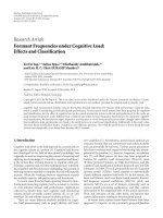
3. Experimental Results
In this section, several results of the simulations on the seg-
mentation of medical and synthetic colour images (Figure 5),
which illustrate the ideas presented in the previous section,
are given.
In order to evaluate the performance of the proposed
algorithm on the segmentation of colour cell images (which
is a challenging problem in this field), the segmentation
results of the datasets are reported. Consequently, a synthetic
image dataset is developed and used for numerical evaluation
purpose.
First the segmentation results in RGB colour space by
applying the proposed method to red, green, and blue colour
features, respectively, are presented. In this case, we find that
the regions are recognized for example in red and green
components but are not identified by the blue component.
This shows the lack of information when using only one
information source and may be explained by the high degree
of correlation among of the three components of the RGB
colour space.
The experimentation is carried out on a medical image
provided by a cancer hospital Figure 2(a) andusedasan
original image. The results are shown in Figures 2(b), 2(c),
and 2(d).

The problem of the incorrectly segmentation is also
illustrated in Figure 2(b), the resulting image has four cells,
while in Figures 2(c) and 2(d) the resulting image by using
homogeneity histogram thresholding has only three and two
cells, respectively.
Comparing the results, we can find that the cells are much
better segmented in (b) than in (c) and (d). Also, the first
resulting image contains some missing features in one of the
cells, which do not exist in the other resulting images. This
demonstrates the necessity of using the fusion process
Also let us compare the performance of our proposed
algorithm to those in other published reports that have
recently been applied to colour images. These include
Zimmermann and Zysno [14], Vannoorenberghe et al. [16],
Ben Chaabane et al. [24], Zhu et al. [17], and Ben Chaabane
et al. [23].
The segmentation results are shown in Figures 3, 4, 6,and
7.
Firstly let us present a colour image that contains two
classes. To highlight its performance let us compare it with
the MMFD [14]andMMFAGD[24] algorithms.
Secondly let us work on more realistic images containing
multiple classes and compare the performance of our
method with other methods that use FCM [23], and HCM
[21] algorithms as tools for the estimation of mass functions
in the Dempster-Shafer evidence theory. Figures 3, 4, 6,and
7 show the obtained results of the proposed method.
6 EURASIP Journal on Advances in Signal Processing
Original image
Calculate the mass functions of

each primitive colour based on the
assumption of Gaussian distribution
Each component image is
divided into sub-regions,
each has a similar colour
Combination of the three
information sources
Final segmentation results
Input the image
Calculate the homogeneity
feature and create the
homogeneity histogram
Apply peak finding algorithm to
the homogeneity histogram, and
perform segmentation in the
homogeneity domain
Calculate the orthogonal sum of
mass functions
Decision
Figure 1: Flowchart of the proposed method.
The original images are artificial, that is, generated with
a user defined classification, and are stored in RGB format.
Each of the primitive colours (red, green, and blue) takes 8
bits and has an intensity range from 0 to 255.
Figure 3 shows a comparison of the results between the
traditional methods MMFD [14], MMFADG [24], and the
proposed method. However, the image shown in Figure 3(b)
represents the original image I where a “Salt and pepper”
noise of D density was added. This affects approximately
(D

× (N ×M)) pixels. The value of D is 0.02.
The final images using the MMFD and MMFAGD
algorithms and the homogeneity for the determination of
mass functions in DS theory are shown in Figures 3(c), 3(d),
and 3(e),respectively.
Comparing Figures 3(c), 3(d),and3(e), one can find that
the cell is much better segmented in (e) than those in (c) and
(d), also the first and the second images contain some holes
in the cell and some pixels were incorrectly segmented. These
do not exist in the correctly segmented image, but after the
redefining process, only a few singularity points are left in the
final image as shown in Figure 3(e).
Accordingly, the dark blue colour of the cell is identified
by the proposed method (Figure 3(e)), but is not seen in
other traditional methods (Figures 3(c) and 3(d)).
It can be seen from Tab l e 1 that 31.77%, 20.44%, and
2.73% of pixels were incorrectly segmented in Figures 3(c),
3(d),and3(e), respectively. However, the two regions are
correctly segmented in Figure 3(e), using the complementary
information provided by the three primitive colours and
consequently a good estimation of mass function by homo-
geneity, even in the presence of a noise (without the filtering
step) is recorded.
In fact, the experimental results indicate that the pro-
posed method, which uses both local and global information
for mass function calculation in DS evidence theory, is
more accurate than the traditional methods in terms of
segmentation quality as denoted by segmentation sensitivity,
see Ta bl e 1 .
In the method based on traditional histogram thresh-

olding [16, 24] only global information is considered in the
histogram analysis.
To provide insights into the proposed method, we
have compared the performance of the proposed method
with those of the corresponding Hard and Fuzzy C-
Means algorithms. The method was also tested on synthetic
images and compared with other existing methods, see
Figure 4.
Figure 4 shows a synthetic input image that contains a
multicomponent object with complicated boundaries and
different component sizes. This figure consists of mainly
six kinds of objects. After applying the HCM and FCM
algorithms for the estimation of the mass function in DS
evidence theory, followed by the data fusion techniques, the
resulting image is divided into only four and five regions,
respectively. But, using the proposed segmentation method,
the resulting image is divided into six regions.
EURASIP Journal on Advances in Signal Processing 7
Table 1: Segmentation sensitivity from MMFD and DS, MMFAGD and DS and homogeneity method and DS for the data set shown in
Figure 5.
MMFD and DS MMFAGD and DS
Homogeneity and DS
(proposed method)
Sensitivity segmentation (%)
Image 1 66.84 72.94 94.23
Image 2 68.23 79.66 97.27
Image 3 72.56 83.19 90.84
Image 4 85.11 88.91 98.11
Image 5 75.42 76.86 96.85
Image 6 63.71 81.45 98.58

Image 7 83.54 93.88 98.36
Image 8 66.78 79.33 95.37
Image 9 75.84 77.85 99.85
Image 10 54.85 75.17 96.97
Image 11 62.74 74.43 81.13
Image 12 45.37 68.45 97.72
(a) (b)
(c) (d)
Figure 2: Segmentation results on a colour image. (a) Original
image (256
×256×3) with gray level spread on the range [0, 255]. (b)
Red resulting image by homogeneity histogram-based method. (c)
Green resulting image by homogeneity histogram-based method.
(d) Blue resulting image by homogeneity histogram-based method.
The selected thresholds are 147, 110, and 194, respectively.
In brief, the experimental results conform to the visu-
alized colour distribution in the objects. However, the new
classes that appeared in Figure 6(d), tend to increase the
size of some regions (yellow regions), and to shrink other
regions (flowers), and some incorrectly segmented pixels are
present in Figure 6(c),suchastheextrabluecontouringin
the bottom centre flower.
The improved experimental results have been achieved
by the proposed method based on the homogeneity his-
togram which can be used to generate a mass function that
has a typical interpretation, that is, the resulting partition
(a) (b)
(c) (d)
(e) (f)
Figure 3: Comparison of the proposed segmentation method with

other existing methods on a medical image (2 classes, 1 cell).
(a) Original image with RGB representation (256
× 256 × 3), (b)
colour cell image disturbed with a “salt and pepper” noise, (c)
segmentation based on MMFD and DS (d) segmentation based on
MMFAGD and DS, (e) segmentation based on homogeneity and
DS, and (f) reference segmented image.
of the data can be interpreted as the compatibilities of the
points with the class prototypes, while the HCM and FCM
methods use only the gray level to determine the degree of
membership of each pixel.
8 EURASIP Journal on Advances in Signal Processing
Table 2: Segmentation sensitivity from HCM and DS, FCM and DS and homogeneity method and DS for the data set shown in Figure 5.
HCMandDS FCMandDS
Homogeneity and DS
(proposed method)
Sensitivity segmentation (%)
Image 1 86.74 89.45 94.23
Image 2 61.82 88.92 97.27
Image 3 73.76 87.25 90.84
Image 4 89.21 96.68 98.11
Image 5 78.62 90.15 96.85
Image 6 72.33 87.78 98.58
Image 7 73.64 96.88 98.36
Image 8 61.48 88.79 95.37
Image 9 73.38 99.63 99.85
Image 10 64.42 79.58 96.97
Image 11 44.93 69.07 81.13
Image 12 56.87 67.31 97.72
(a) (b)

(c) (d)
Figure 4: Comparison of the proposed segmentation method with
other existing methods on a synthetic image (6 classes). (a) Original
image (256
×256×3): colour synthetic image with RGB description,
(b) segmentation based on HCM and DS, (c) segmentation based
on FCM and DS, and (d) segmentation based on homogeneity and
DS.
Comparing Figures 4(b), 4(c),and4(d), one can see that
the different objects of the image are much better segmented
in (d) than those in (b) and (c).
Figures 6 and 7 show other comparison results on a com-
plex medical image. The segmentation results are obtained
using the HCM, the FCM and Homogeneity method.
They correspond, respectively, to Figures 6(b), 6(c),and
6(d) in Figure 6. The cells are exactly and homogeneously
segmented in Figure 6(d), which is not the case of Figures
6(b) and 6(c).
To evaluate the performance of the proposed segmenta-
tion algorithm, its accuracy was recorded.
Figure 5: Data set used in the experiment. Twelve were selected for
a comparison study. The patterns are numbered from 1 through 12,
starting at the upper left-hand corner.
Regarding the accuracy, Tables 1 and 2 list the segmenta-
tion sensitivity of the different methods for the data set used
in the experiment.
The segmentation sensitivity [33, 34] is determined as
follows:
Sens
=

N
pcc
N × M
× 100, (23)
with Sens, N
pcc
, N × M correspond, respectively, to the
segmentation sensitivity (%), number of correctly classified
pixels and dimension of the image. The acquisition of the
correct classified pixels is not a manual process; hence
EURASIP Journal on Advances in Signal Processing 9
(a) (b)
(c) (d)
Figure 6: Comparison of the proposed segmentation method with
other existing methods on a complex medical image (2 classes,
various cells). (a) Original image (256
× 256 × 3): colour medical
image with RGB description, (b) segmentation based on HCM and
DS,(c)segmentationbasedonFCMandDS,and(d)segmentation
based on homogeneity and DS.
(a) (b)
(c) (d)
Figure 7: Comparison of the proposed segmentation method with
other existing methods on a complex medical image (3 classes,
various cells). (a) Original image (256
×256×3): colour cells image
with RGB description, (b) segmentation based on HCM and DS, (c)
segmentation based on FCM and DS, and (d) segmentation based
on homogeneity and DS.
software based on a reference image is run. It consists of a

small program which compares the labels of the obtained
pixels and the reference pixels as shown in Figure 3(f).The
correctly classified pixel denotes a pixel with a label equal to
its corresponding pixel in the reference image. The labeling
of the original image is generated by the user based on the
image used for segmentation.
121110987654321
Image reference
MMFD and DS
MMFAGD and DS
Homogeneity and DS
0
20
40
60
80
100
120
Segmentation sensitivity (%)
Figure 8: Segmentation sensitivity plots using MMFD and DS,
MMFAGD and DS and homogeneity method and DS for the data
set shown in Figure 5.
121110987654321
Image reference
HCM and DS
FCM and DS
Homogeneity and DS
0
20
40

60
80
100
120
Segmentation sensitivity (%)
Figure 9: Segmentation sensitivity plots using HCM and DS, FCM
and DS and homogeneity method and DS for the data set shown in
Figure 5.
In fact, the experimental results presented in Figure 6(d)
are quite consistent with the visualized colour distributions
in the objects, which make it possible to do an accurate
measurement of cell volumes.
Parts (b), (c), and (d) of Figure 7 show other segmenta-
tion results and were obtained using HCM, FCM algorithms,
and the homogeneity method, as used for the DS mass
determination.
In Figure 7(a), only three colours are needed to represent
the colour image (dark blue, blue, and background). In
Figures 7(b) and 7(c), the resulting image has only two
colours. In Figure 7(d), the resulting image has three colours.
The partition resulting by the HCM is less accurate, and
the partition resulting by FCM is not satisfactory either.
The performance of the homogeneity method is quite
acceptable. In fact, one can observe in Figures 7(b) and
7(c) that 13.26% and 10.55% of pixels were incorrectly
segmented for the HCM and FCM methods, respectively.
However, this demonstrates that the mass functions resulting
from the two algorithms, do not always correspond to the
intuitive concept of degree of belonging or compatibility,
10 EURASIP Journal on Advances in Signal Processing

and the generated mass functions do not have a typical
interpretation. Moreover, the HCM and FCM algorithms are
instable in noisy environments. However, errors were largely
reduced when exploiting simultaneously the three images
through the use of the DS fusion method including the
homogeneity histogram.
Indeed, only 5.77% of pixels were incorrectly segmented
in Figure 7(d). This good performance between these meth-
ods can also be easily assessed by visually comparing the
segmentation results.
The segmentation sensitivity values reported in Tables 1
and 2 are plotted in Figures 8 and 9,respectively.
Figure 8 shows two segmentation sensitivity plots using
traditional methods such as MMFD and MMFAGD com-
pared with the proposed method plot.
Figure 9 shows two other segmentation sensitivity plots
using automatic methods such as HCM and FCM compared
with the proposed method plot.
As seen on both Figures 8 and 9, the proposed method
plot is clearly located on the top of the other methods plots.
Referring to segmentation sensitivity plots given in
Figure 9, one observes that 27.67%, 12.22%, and 1.42% of
pixels were incorrectly segmented in Figures 6(b), 6(c),and
6(d), respectively. Comparing Figures 6(b) and 6(c) with
Figure 6(d), the resulting image by the proposed method is
much clearer than the one given by the HCM and FCM
methods.
4. Conclusion
In this paper, we have proposed a new method for colour
image segmentation based on homogeneity histogram

thresholding and data fusion techniques. In the first phase,
uniform regions are identified in each primitive colour via
a thresholding operation on a newly defined homogeneity
histogram. Then, the DS combination rule and decision are
applied to fuse the three primitive colours.
The results obtained show the generic and robust
character of the method in the sense that the local and
global information were involved in the fusion process. On
the other hand, in the estimation of mass function, we have
used the local and global information. The results obtained
demonstrated the significant improved performance in seg-
mentation. The proposed method can be useful for colour
image segmentation.
Nevertheless, there are some drawbacks to our proposed
method. The used image models are mainly based on some
a priori knowledge such as the mean and the standard
deviation of each region of the image to be segmented. Also,
in all our work, we have considered only one image for
each application, whereas, many realizations of the same
image fused together may be very helpful to the segmentation
process. Furthermore, the research of other optimal models
to estimate the mass functions in the Dempster-Shafer
evidence theory and the fusion of imperfect information
coming from different colour images are an important
aspect of our present work. Also, the proposed method
assumes that we have a reference image, which should be
labelled by the user for comparison purposes. In practice,
this is not realisable; hence advanced intelligent software for
classification based on the Kohonen Neural Network may be
used in parallel with the proposed segmentation procedure

to avoid the manually labelling of the image by the user.
References
[1] E. Navon, O. Miller, and A. Averbuch, “Color image segmen-
tation based on adaptive local thresholds,” Image and Vision
Computing, vol. 23, no. 1, pp. 69–85, 2005.
[2] S. Kasaei and M. Hasanzadeh, “Fuzzy image segmentation
using membership connectedness,” EURASIP Journal on
Advances in Signal Processing, vol. 2008, Article ID 417293, 13
pages, 2008.
[3] H.D.Cheng,X.H.Jiang,Y.Sun,andJ.Wang,“Colorimage
segmentation: advances and prospects,” Pattern Recognition,
vol. 34, no. 12, pp. 2259–2281, 2001.
[4] R. Etienne-Cummings, P. Pouliquen, and M. A. Lewis, “A
vision chip for color segmentation and pattern matching,”
EURASIP Journal on Applied Signal Processing, vol. 2003, no.
7, pp. 703–712, 2003.
[5] X. Gao, K. Hong, P. Passmore, L. Podladchikova, and D.
Shaposhnikov, “Colour vision model-based approach for
segmentation of traffic signs,” EURASIP Journal on Image and
Video Processing, vol. 2008, Article ID 386705, 7 pages, 2008.
[6] R. Bradley, “A unified Bayesian decision theory,” Theory and
Decision, vol. 63, no. 3, pp. 233–263, 2007.
[7] I. Bloch and H. Maitre, “Fusion of image information under
imprecision,” in Aggregation and Fusion of Imperfect Informa-
tion, B. Bouchon-Meunier, Ed., Series studies in fuzziness,
Physical Verlag, pp. 189–213, Springer, 1997.
[8] S L. Dong, J M. Wei, T. Xing, and H T. Liu, “Constraint-
based fuzzy optimization data fusion for sensor network
localization,” in Proceedings of the 2nd International Conference
on Semantics Knowledge and Grid (SKG ’06), p. 59, November

2006.
[9] C. Lucas and B. N. Araabi, “Generalization of the Dempster-
Shafer theory: a fuzzy-valued measure,” IEEE Transactions on
Fuzzy Systems, vol. 7, no. 3, pp. 255–270, 1999.
[10] D. Dubois and H. Prade, “Possibility theory and its applica-
tions: a retrospective and prospective view,” in Proceedings of
the IEEE International Conference on Fuzzy Systems, vol. 1, pp.
5–11, May 2003.
[11] A. P. Dempster, “Upper and lower probabilities induced by
multivalued mapping,” Annals of Mathematical Statistics, vol.
38, pp. 325–339, 1967.
[12] G. Shafer, A Mathematical Theory of Evidence, Princeton
University Press, 1976.
[13] T. Denœux, “A k-nearest neighbor classification rule based on
Dempster-Shafer theory,” IEEE Transactions on Systems, Man
&Cybernetics, vol. 25, no. 5, pp. 804–813, 1995.
[14] H J. Zimmermann and P. Zysno, “Quantifying vagueness in
decision models,” European Journal of Operational Research,
vol. 22, no. 2, pp. 148–158, 1985.
[15] K. Raghu and J. M. Keller, “A possibilistic method to
clustering,” IEEE Transactions on Fuzzy Systems,vol.1,no.2,
1993.
[16] P. Vannoorenberghe, O. Colot, and D. De Brucq, “Color
image segmentation using Dempster-Shafer’s theory,” IEEE
International Conference on Image Processing (ICIP ’99), vol.
4, pp. 300–304, October 1999.
EURASIP Journal on Advances in Signal Processing 11
[17] Y. M. Zhu, L. Bentabet, O. Dupuis, V. Kaftandjian, D.
Babot, and M. Rombaut, “Automatic determination of mass
functions in Dempster-Shafer theory using fuzzy c-means and

spatial neighborhood information for image segmentation,”
Optical Engineering, vol. 41, no. 4, pp. 760–770, 2002.
[18] R. R. Yager, “Class of fuzzy measures generated from a
Dempster-Shafer belief structure,” International Journal of
Intelligent Systems, vol. 14, no. 12, pp. 1239–1247, 1999.
[19] J. C. Bezdek, Pattern Recognition with Fuzzy Objective Function
Algorithms, Plenum Press, New York, NY, USA, 1981.
[20] M. N. Ahmed, S. M. Yamany, N. Mohamed, A. A. Farag, and T.
Moriarty, “A modified fuzzy C-means algorithm for bias field
estimation and segmentation of MRI data,” IEEE Transactions
on Medical Imaging, vol. 21, no. 3, pp. 193–199, 2002.
[21] R. Duda and P. Hart, Pattern Classification and Scene Analysis,
John Wiley & Sons, New York, NY, USA, 1973.
[22]L.Gautier,A.Taleb-Ahmed,M.Rombaut,J.G.Postaire,
and H. Leclet, “Help to decison of segmentation of pictures
by Dempster-Shafer theory: application to MRI sequence,”
Editions Scientifiques et Medicales Elsevier SAS,vol.22,no.6,
pp. 378–392, 2001.
[23] S. Ben Chaabane, M. Sayadi, F. Fnaiech, and E. Brassart,
“Dempster-Shafer evidence theory for image segmentation:
application in cells images,” International Journal of Signal
Processing, vol. 5, no. 1, 2009.
[24] S. Ben Chaabane, M. Sayadi, F. Fnaiech, and E. Brassart,
“Color image segmentation based on Dempster-Shafer evi-
dence theory,” in Proceedings of the Mediterranean Electrotech-
nical Conference (MELECON ’08), pp. 862–866, 2008.
[25] H. D. Cheng, C. H. Chen, H. H. Chiu, and H. Xu, “Fuzzy
homogeneity approach to multilevel thresholding,” IEEE
Transactions on Image Processing, vol. 7, no. 7, pp. 1084–1088,
1998.

[26] E. Littmann and H. Ritter, “Adaptive color segmentation—a
comparison of neural and statistical methods,” IEEE Transac-
tions on Neural Networks, vol. 8, no. 1, pp. 175–185, 1997.
[27] M. Sezgin and B. Sankur, “Survey over image thresholding
techniques and quantitative performance evaluation,” Journal
of Electronic Imaging, vol. 13, no. 1, pp. 146–168, 2004.
[28] H D. Cheng and Y. Sun, “A hierarchical approach to color
image segmentation using homogeneity,” IEEE Transactions on
Image Processing, vol. 9, no. 12, pp. 2071–2082, 2000.
[29] H. D. Cheng, X. H. Jiang, and J. Wang, “Color image
segmentation based on homogram thresholding and region
merging,” Pattern Recognition, vol. 35, no. 2, pp. 373–393,
2002.
[30] R. C. Gonzalez and P. Wintz, Digital Image Processing,
Addison-Wesley, Reading, Mass, USA, 1987.
[31] M. Heath, S. Sarkar, T. Sanocki, and K. Bowyer, “Comparison
of edge detectors: a methodology and initial study,” in Pro-
ceedings of the IEEE Computer Society Conference on Computer
Vision and Pattern Recognition, pp. 143–148, 1996.
[32] G. Liu and R. M. Haralick, “Assignment problem in edge
detection performance evaluation,” in Proceedings of the IEEE
Computer Society Conference on Computer Vision and Pattern
Recognition, vol. 1, pp. 26–31, 2000.
[33]V.Grau,A.U.J.Mewes,M.Alca
˜
niz, R. Kikinis, and S. K.
Warfield, “Improved watershed transform for medical image
segmentation using prior information,” IEEE Transactions on
Medical Imaging, vol. 23, no. 4, pp. 447–458, 2004.
[34] R.O.Duda,P.E.Hart,andD.G.Sork,Pattern Classification,

Wiley-Interscience, New York, NY, USA, 2000.