báo cáo hóa học:" Research Article An Open Framework for Rapid Prototyping of Signal Processing Applications" pdf

Hindawi Publishing Corporation
EURASIP Journal on Embedded Systems
Volume 2009, Article ID 598529, 13 pages
doi:10.1155/2009/598529

Research Article
An Open Framework for Rapid Prototyping of
Signal Processing Applications
Maxime Pelcat,1 Jonathan Piat,1 Matthieu Wipliez,1 Slaheddine Aridhi,2
and Jean-Francois Nezan1
¸
1 IETR/Image

and Remote Sensing Group, CNRS UMR 6164/INSA Rennes, 20, avenue des Buttes de Coăsmes,
e
35043 Rennes Cedex, France
2 HPMP Division, Texas Instruments, 06271 Villeneuve Loubet, France
Correspondence should be addressed to Maxime Pelcat,
Received 27 February 2009; Revised 7 July 2009; Accepted 14 September 2009
Recommended by Markus Rupp
Embedded real-time applications in communication systems have significant timing constraints, thus requiring multiple
computation units. Manually exploring the potential parallelism of an application deployed on multicore architectures is greatly
time-consuming. This paper presents an open-source Eclipse-based framework which aims to facilitate the exploration and
development processes in this context. The framework includes a generic graph editor (Graphiti), a graph transformation library
(SDF4J) and an automatic mapper/scheduler tool with simulation and code generation capabilities (PREESM). The input of the
framework is composed of a scenario description and two graphs, one graph describes an algorithm and the second graph describes
an architecture. The rapid prototyping results of a 3GPP Long-Term Evolution (LTE) algorithm on a multicore digital signal
processor illustrate both the features and the capabilities of this framework.
Copyright © 2009 Maxime Pelcat et al. This is an open access article distributed under the Creative Commons Attribution License,
which permits unrestricted use, distribution, and reproduction in any medium, provided the original work is properly cited.

1. Introduction
The recent evolution of digital communication systems
(voice, data, and video) has been dramatic. Over the last two
decades, low data-rate systems (such as dial-up modems, first
and second generation cellular systems, 802.11 Wireless local
area networks) have been replaced or augmented by systems
capable of data rates of several Mbps, supporting multimedia
applications (such as DSL, cable modems, 802.11b/a/g/n
wireless local area networks, 3G, WiMax and ultra-wideband
personal area networks).
As communication systems have evolved, the resulting
increase in data rates has necessitated a higher system algorithmic complexity. A more complex system requires greater
flexibility in order to function with different protocols in
different environments. Additionally, there is an increased
need for the system to support multiple interfaces and
multicomponent devices. Consequently, this requires the
optimization of device parameters over varying constraints
such as performance, area, and power. Achieving this
device optimization requires a good understanding of the

application complexity and the choice of an appropriate
architecture to support this application.
An embedded system commonly contains several processor cores in addition to hardware coprocessors. The
embedded system designer needs to distribute a set of signal
processing functions onto a given hardware with predefined
features. The functions are then executed as software code
on target architecture; this action will be called a deployment
in this paper. A common approach to implement a parallel
algorithm is the creation of a program containing several
synchronized threads in which execution is driven by the

scheduler of an operating system. Such an implementation
does not meet the hard timing constraints required by realtime applications and the memory consumption constraints
required by embedded systems [1]. One-time manual
scheduling developed for single-processor applications is
also not suitable for multiprocessor architectures: manual
data transfers and synchronizations quickly become very
complex, leading to wasted time and potential deadlocks.


2
Furthermore, the task of finding an optimal deployment of
an algorithm mapped onto a multicomponent architecture
is not straightforward. When performed manually, the result
is inevitably a suboptimal solution. These issues raise the
need for new methodologies, which allow the exploration of
several solutions, to achieve a more optimal result.
Several features must be provided by a fast prototyping
process: description of the system (hardware and software),
automatic mapping/scheduling, simulation of the execution, and automatic code generation. This paper draws on
previously presented works [2–4] in order to generate a
more complete rapid prototyping framework. This complete
framework is composed of three complementary tools based
on Eclipse [5] that provide a full environment for the
rapid prototyping of real-time embedded systems: Parallel
and Real-time Embedded Executives Scheduling Method
(PREESM), Graphiti and Synchronous Data Flow for Java
(SDF4J). This framework implements the methodology
Algorithm-Architecture Matching (AAM), which was previously called Algorithm-Architecture Adequation (AAA) [6].
The focus of this rapid prototyping activity is currently
static code mapping/scheduling but dynamic extensions are

planned for future generations of the tool.
From the graph descriptions of an algorithm and of
an architecture, PREESM can find the right deployment,
provide simulation information, and generate a framework
code for the processor cores [2]. These rapid prototyping
tasks can be combined and parameterized in a workflow.
In PREESM, a workflow is defined as an oriented graph
representing the list of rapid prototyping tasks to execute
on the input algorithm and architecture graphs in order
to determine and simulate a given deployment. A rapid
prototyping process in PREESM consists of a succession of
transformations. These transformations are associated in a
data flow graph representing a workflow that can be edited in
a Graphiti generic graph editor. The PREESM input graphs
may also be edited using Graphiti. The PREESM algorithm
models are handled by the SDF4J library. The framework can
be extended by modifying the workflows or by connecting
new plug-ins (for compilation, graph analyses, and so on).
In this paper, the differences between the proposed
framework and related works are explained in Section 2.
The framework structure is described in Section 3. Section 4
details the features of PREESM that can be combined by
users in workflows. The use of the framework is illustrated by
the deployment of a wireless communication algorithm from
the 3rd Generation Partnership Project (3GPP) Long-Term
Evolution (LTE) standard in Section 5. Finally, conclusions
are given in Section 6.

2. State of the Art of Rapid Prototyping and
Multicore Programming

There exist numerous solutions to partition algorithms
onto multicore architectures. If the target architecture is
homogeneous, several solutions exist which generate multicore code from C with additional information (OpenMP
[7], CILK [8]). In the case of heterogeneous architectures,

EURASIP Journal on Embedded Systems
languages such as OpenCL [9] and the Multicore Association
Application Programming Interface (MCAPI [10]) define
ways to express parallel properties of a code. However,
they are not currently linked to efficient compilers and
runtime environments. Moreover, compilers for such languages would have difficulty in extracting and solving the
bottlenecks of the implementation that appear inherently in
graph descriptions of the architecture and the algorithm.
The Poly-Mapper tool from PolyCore Software [11]
offers functionalities similar to PREESM but, in contrast
to PREESM, its mapping/scheduling is manual. Ptolemy II
[12] is a simulation tool that supports many models of
computation. However, it also has no automatic mapping
and currently its code generation for embedded systems
focuses on single-core targets. Another family of frameworks
existing for data flow based programming is based on
CAL [13] language and it includes OpenDF [14]. OpenDF
employs a more dynamic model than PREESM but its
related code generation does not currently support multicore
embedded systems.
Closer to PREESM are the Model Integrated Computing
(MIC [15]), the Open Tool Integration Environment (OTIE
[16]), the Synchronous Distributed Executives (SynDEx
[17]), the Dataflow Interchange Format (DIF [18]), and
SDF for Free (SDF3 [19]). Both MIC and OTIE can not

be accessed online. According to literature, MIC focuses
on the transformation between algorithm domain-specific
models and metamodels while OTIE defines a single system
description that can be used during the whole signal
processing design cycle.
DIF is designed as an extensible repository of representation, analysis, transformation, and scheduling of data
flow language. DIF is a Java library which allows the user
to go from graph specification using the DIF language to
C code generation. However, the hierarchical Synchronous
Data Flow (SDF) model used in the SDF4J library and
PREESM is not available in DIF.
SDF3 is an open-source tool implementing some data
flow models and providing analysis, transformation, visualization, and manual scheduling as a C++ library. SDF3
implements the Scenario Aware Data Flow (SADF [20]), and
provides Multiprocessor System-on-Chip (MP-SoC) binding/scheduling algorithm to output MP-SoC configuration
files.
SynDEx and PREESM are both based on the AAM
methodology [6] but the tools do not provide the same
features. SynDEx is not an open source, it has its own model
of computation that does not support schedulability analysis,
and code generation is possible but not provided with the
tool. Moreover, the architecture model of SynDEx is at a too
high level to account for bus contentions and DMA used
in modern chips (multicore processors of MP-SoC) in the
mapping/scheduling.
The features that differentiate PREESM from the related
works and similar tools are
(i) The tool is an open source and accessible online;
(ii) the algorithm description is based on a single wellknown and predictable model of computation;

EURASIP Journal on Embedded Systems

SDF4J
Generic graph
editor eclipse
plug-in

3

Data flow graph
transformation library

PREESM

Scheduler

Graph
transformation

Graphiti

Rapid prototyping
eclipse plug-ins

Code
generator

Core
Eclipse framework

Figure 1: An Eclipse-based Rapid Prototyping Framework.

(iii) the mapping and the scheduling are totally automatic;
(iv) the functional code for heterogeneous multicore
embedded systems can be generated automatically;
(v) the algorithm model provides a helpful hierarchical encapsulation thus simplifying the mapping/scheduling [3].
The PREESM framework structure is detailed in the next
section.

3. An Open-Source Eclipse-Based Rapid
Prototyping Framework
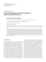
3.1. The Framework Structure. The framework structure is
presented in Figure 1. It is composed of several tools to
increase reusability in several contexts.
The first step of the process is to describe both the target
algorithm and the target architecture graphs. A graphical
editor reduces the development time required to create,
modify and edit those graphs. The role of Graphiti [21] is
to support the creation of algorithm and architecture graphs
for the proposed framework. Graphiti can also be quickly
configured to support any type of file formats used for
generic graph descriptions.
The algorithm is currently described as a Synchronous
Data Flow (SDF [22]) Graph. The SDF model is a good
solution to describe algorithms with static behavior. The
SDF4J [23] is an open-source library providing usual
transformations of SDF graphs in the Java programming
language. The extensive use of SDF and its derivatives in
the programming model community led to the development

of SDF4J as an external tool. Due to the greater specificity
of the architecture description compared to the algorithm
description, it was decided to perform the architecture
transformation inside the PREESM plug-ins.
The PREESM project [24] involves the development of a
tool that performs the rapid prototyping tasks. The PREESM
tool uses the Graphiti tool and SDF4J library to design
algorithm and architecture graphs and to generate their
transformations. The PREESM core is an Eclipse plug-in that
executes sequences of rapid prototyping tasks or workflows.
The tasks of a workflow are delegated to PREESM plugins. There are currently three PREESM plug-ins: the graph

transformation plug-in, the scheduler plug-in, and the codegeneration plug-in.
The three tools of the framework are detailed in the next
sections.
3.2. Graphiti: A Generic Graph Editor for Editing Architectures,
Algorithms and Workflows. Graphiti is an open-source plugin for the Eclipse environment that provides a generic graph
editor. It is written using the Graphical Editor Framework
(GEF). The editor is generic in the sense that any type
of graph may be represented and edited. Graphiti is used
routinely with the following graph types and associated file
formats: CAL networks [13, 25], a subset of IP-XACT [26],
GraphML [27] and PREESM workflows [28].
3.2.1. Overview of Graphiti. A type of graph is registered
within the editor by a configuration. A configuration is an
XML (Extensible Markup Language [29]) file that describes
(1) the abstract syntax of the graph (types of vertices
and edges, and attributes allowed for objects of each
type);
(2) the visual syntax of the graph (colors, shapes, etc.);

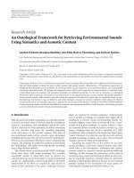
(3) transformations from the file format in which the
graph is defined to Graphiti’s XML file format G, and
vice versa (Figure 2);
Two kinds of input transformations are supported, from
XML to XML and from text to XML (Figure 2). XML is
transformed to XML with Extensible Stylesheet Language
Transformation (XSLT [30]), and text is parsed to its Concrete Syntax Tree (CST) represented in XML according to a
LL(k) grammar by the Grammatica [31] parser. Similarly,
two kinds of output transformations are supported, from
XML to XML and from XML to text.
Graphiti handles attributed graphs [32]. An attributed
graph is defined as a directed multigraph G = (V , E, μ) with
V the set of vertices, E the multiset of edges (there can be
more than one edge between any two vertices). μ is a function
μ : ({G} ∪ V ∪ E) × A → U that associates instances with
attributes from the attribute name set A and values from U,
the set of possible attribute values. A built-in type attribute
is defined so that each instance i ∈ {G} ∪ V ∪ E has a type
t = μ(i, type), and only admits attributes from a set At ⊂ A


4

EURASIP Journal on Embedded Systems
XML
Text

Parsing

XSLT

transformations

XML
CST

G

(a)
G

XML

XSLT
transformations

Text
(b)

Figure 2: Input/output with Graphiti’s XML format G.

do something
acc
produce

<vertexType name=“node”>
<attributes>
<color red=“163” green=“0” blue=“85”/>
<shape name=“roundedBox”/>
<size width=“40” height=“40”/>
</attributes>

type=“java.lang.String”
default=“ ”/>
type=“java.util.List”>
<element value=“0”/>
</parameter>
</parameters>
</vertexType>

out

in

out

consume

Figure 4: The type of vertices of the graph shown in Figure 3.

in

Figure 3: A sample graph.

given by At = τ(t). Additionally, a type t has a visual syntax
σ(t) that defines its color, shape, and size.
To edit a graph, the user selects a file and the matching
configuration is computed based on the file extension. The
transformations defined in the configuration file are then

applied to the input file and result in a graph defined in
Graphiti’s XML format G as shown in Figure 2. The editor
uses the visual syntax defined by σ in the configuration to
draw the graph, vertices, and edges. For each instance of type
t the user can edit the relevant attributes allowed by τ(t)
as defined in the configuration. Saving a graph consists of
writing the graph in G, and transforming it back to the input
file’s native format.
3.2.2. Editing a Configuration for a Graph Type. To create a
configuration for the graph represented in Figure 3, a node (a
single type of vertex) must be defined. A node has a unique
identifier called id, and accepts a list of values initially equal to
[0] (Figure 4). Additionally, ports need to be specified on the
edges, so the configuration describes an edgeType element
(Figure 5) that carries sourcePort and targetPort parameters
to store an edge’s source and target ports, respectively, such
as acc, in, and out in Figure 3.
Graphiti is a stand-alone tool, totally independent of
PREESM. However, Graphiti generates workflow graphs,
IP-XACT and GraphML files that are the main inputs of
PREESM. The GraphML files contain the algorithm model.
These inputs are loaded and stored in PREESM by the SDF4J
library. This library, discussed in the next section, executes
the graph transformations.
3.3. SDF4J: A Java Library for Algorithm Data Flow Graph
Transformations. SDF4J is a library defining several Data
Flow oriented graph models such as SDF and Directed
Acyclic Graph (DAG [33]). It provides the user with several
classic SDF transformations such as hierarchy flattening, and

<edgeType name=“edge”>
<attributes>
<directed value=“true”/>
</attributes>

type=“java.lang.String”
default=“ ”/>
type=“java.lang.String”
default=“ ”/>
</parameters>
</vertexType>
Figure 5: The type of edges of the graph shown in Figure 3.

SDF to Homogeneous SDF (HSDF [34]) transformations
and some clustering algorithms. This library also gives the
possibility to expand optimization templates. It defines its
own graph representation based on the GraphML standard
and provides the associated parser and exporter class. SDF4J
is freely available (GPL license) for download.
3.3.1. SDF4J SDF Graph model. An SDF graph is used
to simplify the application specifications. It allows the
representation of the application behavior at a coarse grain
level. This data flow representation models the application
operations and specifies the data dependencies between these
operations.
An SDF graph is a finite directed, weighted graph G =<
V , E, d, p, c > where:
(i) V is the set of nodes. A node computes an input data

stream and outputs the result;
(ii) E ⊆ V × V is the edge set, representing channels
which carry data streams;
(iii) d : E → N ∪ {0} is a function with d(e) the number
of initial tokens on an edge e;
(iv) p : E → N is a function with p(e) representing the
number of data tokens produced at e’s source to be
carried by e;


EURASIP Journal on Embedded Systems
op1 3

2 op 2
2

3

4

5

op4

1

4
2 op3 2

op1 3

1

op2

1
op1 1

op2
1 op
2

1

Figure 6: A SDF graph.

(v) c : E → N is a function with c(e) representing the
number of data tokens consumed from e by e’s sink
node;
This model offers strong compile-time predictability
properties, but has limited expressive capability. The SDF
implementation enabled by the SDF4J supports the hierarchy
defined in [3] which increases the model expressiveness. This
specific implementation is straightforward to the programmer and allows user-defined structural optimizations. This
model is also intended to lead to a better code generation
using common C patterns like loop and function calls. It is
highly expandable as the user can associate any properties
to the graph components (edge, vertex) to produce a
customized model.
3.3.2. SDF4J SDF Graph Transformations. SDF4J implements

several algorithms intended to transform the base model or
to optimize the application behavior at different levels.
(i) The hierarchy flattening transformation aims to flatten
the hierarchy (remove hierarchy levels) at the chosen
depth in order to later extract as much as possible
parallelism from the designer’s hierarchical description.
(ii) The HSDF transformation (Figure 7) transforms the
SDF model to an HSDF model in which the amount
of tokens exchanged on edges are homogeneous
(production = consumption). This model reveals
all the potential parallelism in the application but
dramatically increases the amount of vertices in the
graph.
(iii) The internalization transformation based on [35]
is an efficient clustering method minimizing the
number of vertices in the graph without decreasing
the potential parallelism in the application.
(iv) The SDF to DAG transformation converts the SDF or
HSDF model to the DAG model which is commonly
used by scheduling methods [33].
3.4. PREESM: A Complete Framework for Hardware and Software Codesign. In the framework, the role of the PREESM
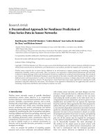
tool is to perform the rapid prototyping tasks. Figure 8
depicts an example of a classic workflow which can be
executed in the PREESM tool. As seen in Section 3.3, the
data flow model chosen to describe applications in PREESM
is the SDF model. This model, described in [22], has the
great advantage of enabling the formal verification of static
schedulability. The typical number of vertices to schedule in

1

op2

Figure 7: A SDF graph and its HSDF transformation.

PREESM is between one hundred and several thousands. The
architecture is described using IP-XACT language, an IEEE
standard from the SPIRIT consortium [26]. The typical size
of an architecture representation in PREESM is between a
few cores and several dozen cores. A scenario is defined as a
set of parameters and constraints that specify the conditions
under which the deployment will run.
As can be seen in Figure 8, prior to entering the
scheduling phase, the algorithm goes through three transformation steps: the hierarchy flattening transformation,
the HSDF transformation, and the DAG transformation
(see Section 3.3.2). These transformations prepare the graph
for the static scheduling and are provided by the Graph
Transformation Module (see Section 4.1). Subsequently, the
DAG—converted SDF graph—is processed by the scheduler
[36]. As a result of the deployment by the scheduler, a
code is generated and a Gantt chart of the execution is
displayed. The generated code consists of scheduled function
calls, synchronizations, and data transfers between cores. The
functions themselves are handwritten.
The plug-ins of the PREESM tool implement the rapid
prototyping tasks that a user can add to the workflows. These
plug-ins are detailed in next section.

4. The Current Features of PREESM
4.1. The Graph Transformation Module. In order to generate

an efficient schedule for a given algorithm description, the
application defined by the designer must be transformed.
The purpose of this transformation is to reveal the potential
parallelism of the algorithm and simplify the work of the
task scheduler. To provide the user with flexibility while
optimizing the design, the entire graph transformation
provided by the SDF4J library can be instantiated in a
workflow with parameters allowing the user to control each
of the three transformations. For example, the hierarchical
flattening transformation can be configured to flatten a
given number of hierarchy levels (depth) in order to keep
some of the user hierarchical construction and to maintain
the amount of vertices to schedule at a reasonable level.
The HSDF transformation provides the scheduler with a
graph of high potential parallelism as all the vertices of the
SDF graph are repeated according to the SDF graph’s basic
repetition vector. Consequently, the number of vertices to
schedule is larger than in the original graph. The clustering
transformation prepares the algorithm for the scheduling
process by grouping vertices according to criteria such as
strong connectivity or strong data dependency between


6

EURASIP Journal on Embedded Systems

Graphiti editor
Architecture
editor

Algorithm
editor

Scenario
editor

Hierarchical
SDF

Scenario

IP-XACT

Hierarchy flattening
SDF
HSDF transformation
HSDF
SDF to DAG transformation
DAG
Mapping /scheduling
DAG + implementation
information

Gantt chart

Code

Code generation
PREESM framework

Figure 8: Example of a workflow graph: from SDF and IP-XACT descriptions to the generated code.

vertices. The grouped vertices are then transformed into a
hierarchical vertex which is then treated as a single vertex
in the scheduling process. This vertex grouping reduces the
number of vertices to schedule, speeding up the scheduling
process. The user can freely use available transformations in
his workflow in order to control the criteria for optimizing
the targeted application and architecture.
As can be seen in the workflow displayed in Figure 8,
the graph transformation steps are followed by the static
scheduling step.
4.2. The PREESM Static Scheduler. Scheduling consists of
statically distributing the tasks that constitute an application
between available cores in a multicore architecture and
minimizing parameters such as final latency. This problem
has been proven to be NP-complete [37]. A static scheduling
algorithm is usually described as a monolithic process, and
carries out two distinct functionalities: choosing the core to
execute a specific function and evaluating the cost of the
generated solutions.
The PREESM scheduler splits these functionalities into
three submodules [4] which share minimal interfaces: the
task scheduling, the edge scheduling, and the Architecture
Benchmark Computer (ABC) submodules. The task scheduling submodule produces a scheduling solution for the
application tasks mapped onto the architecture cores and
then queries the ABC submodule to evaluate the cost of the

proposed solution. The advantage of this approach is that any

task scheduling heuristic may be combined with any ABC
model, leading to many different scheduling possibilities. For
instance, an ABC minimizing the deployment memory or
energy consumption can be implemented without modifying
the task scheduling heuristics.
The interface offered by the ABC to the task scheduling
submodule is minimal. The ABC gives the number of available cores, receives a deployment description and returns
costs to the task scheduling (infinite if the deployment is
impossible). The time keeper calculates and stores timings
for the tasks and the transfers when necessary for the ABC.
The ABC needs to schedule the edges in order to calculate
the deployment cost. However, it is not designed to make
any deployment choices; this task is delegated to the edge
scheduling submodule. The router in the edge scheduling
submodule finds potential routes between the available cores.
The choice of module structure was motivated by
the behavioral commonality of the majority of scheduling
algorithms (see Figure 9).
4.2.1. Scheduling Heuristics. Three algorithms are currently
coded, and are modified versions of the algorithms described
in [38].
(i) A list scheduling algorithm schedules tasks in the
order dictated by a list constructed from estimating
a critical path. Once a mapping choice has been


EURASIP Journal on Embedded Systems
made, it will never be modified. This algorithm is
fast but has limitations due to this last property.
List scheduling is used as a starting point for other

refinement algorithms.
(ii) The FAST algorithm is a refinement of the list
scheduling solution which uses probabilistic hops. It
changes the mapping choices of randomly chosen
tasks; that is, it associates these tasks to another
processing unit. It runs until stopped by the user
and keeps the best latency found. The algorithm is
multithreaded to exploit the multicore parallelism of
a host computer.
(iii) A genetic algorithm is coded as a refinement of the
FAST algorithm. The n best solutions of FAST are
used as the base population for the genetic algorithm.
The user can stop the processing at any time while
retaining the last best solution. This algorithm is also
multithreaded.
The FAST algorithm has been developed to solve complex
deployment problems. In the original heuristic, the final
order of tasks to schedule, as defined by the list scheduling
algorithm, was not modified by the FAST algorithm. The
FAST algorithm only modifies the mapping choices of the
tasks. In large-scale applications, the initial order of the
tasks performed by the list scheduling algorithm becomes
occasionally suboptimal. In the modified version of the FAST
scheduling algorithm, the ABC recalculates the final order of
a task when the heuristic maps a task to a new core. The task
switcher algorithm used to recalculate the order simply looks
for the earliest appropriately sized hole in the core schedule
for the mapped task (see Figure 10).
4.2.2. Scheduling Architecture Model. The current architecture representation was driven by the need to accurately
model multicore architectures and hardware coprocessors

with intercores message-passing communication. This communication is handled in parallel to the computation using
Direct Memory Access (DMA) modules. This model is
currently used to closely simulate the Texas Instruments
TMS320TCI6487 processor (see Section 5.3.2). The model
will soon be extended to shared memory communications
and more complex interconnections. The term operator
represents either a processor core or a hardware coprocessor.
Operators are linked by media, each medium representing a
bus and the associated DMA. The architectures can be either
homogeneous (with all operators and media identical) or
heterogeneous. For each medium, the user defines a DMA
set up time and a bus data rate. As shown in Figure 9,
the architecture model is only processed in the scheduler
by the ABC and not by the heuristic and edge scheduling
submodules.
4.2.3. Architecture Benchmark Computer. Scheduling often
requires much time. Testing intermediate solutions with
precision is an especially time-consuming operation. The
ABC submodule was created by reusing the useful concept
of time scalability introduced in SystemC Transaction Level

7

DAG

Task scheduling

IP-XACT + scenario
Number of cores
Architecture

Task schedule
benchmark
computer (ABC)
Time keeper

Scheduler
Edge scheduling

Cost
Task schedule

Router

Edge
schedule

Figure 9: Scheduler module structure.

Modeling (TLM) [39]. This language defines several levels of
system temporal simulation, from untimed to cycle-accurate
precision. This concept motivated the development of several
ABC latency models with different timing precisions. Three
ABC latency models are currently coded (see Figure 11).
(i) The loosely-timed model takes into account task and
transfer times but no transfer contention.
(ii) The approximately-timed model associates each intercore communication medium with its constant rate
and simulates contentions.
(iii) The accurately-timed model adds set up times which
simulate the duration necessary to initialize a parallel
transfer controller like Texas Instruments Enhanced

Direct Memory Access (EDMA [40]). This set up
time is scheduled in the core which sends the transfer.
The task and architecture properties feeding the ABC
submodule are evaluated experimentally, and include media
data rate, set up times, and task timings. ABC models
evaluating parameters other than latency are planed in
order to minimize memory size, memory accesses, cadence
(i.e., average runtime), and so on. Currently, only latency
is minimized due to the limitations of the list scheduling
algorithms: these costs cannot be evaluated on partial
deployments.
4.2.4. Edge Scheduling Submodule. When a data block is
transferred from one operator to another, transfer tasks are
added and then mapped to the corresponding medium. A
route is associated with each edge carrying data from one
operator to another, which possibly may go through several
other operators. The edge scheduling submodule routes the
edges and schedules their route steps. The existing routing
process is basic and will be developed further once the
architecture model has been extended. Edge scheduling can
be executed with different algorithms of varying complexity,
which results in another level of scalability. Currently, two
algorithms are implemented:
(i) the simple edge scheduler follows the scheduling order
given by the task list provided by the list scheduling
algorithm;


8

EURASIP Journal on Embedded Systems

IP-XACT + scenario

DAG

Edge scheduling
Scheduler

Genetic algorithms

FAST

Latency/cadence/memory driven

Scheduler

Task scheduling

Edge scheduling

IP-XACT scenario
Architecture benchmark computer (ABC)

List scheduling

Only latency-driven

ACCURATE

Cadence

ABC

Memory

DAG
Task scheduling

Accurately-timed Approximately-timed Loosely-timed
Bus contention
+ setup times

Bus contention

FAST

ACCURATE

Figure 10: Switchable scheduling heuristics.

Unscheduled
communication

FAST

Figure 11: Switchable ABC models.

(ii) the switching edge scheduler reuses the task switcher
algorithm discussed in Section 4.2.1 for edge scheduling. When a new communication edge needs to be

scheduled, the algorithm looks for the earliest hole of
appropriate size in the medium schedule.
The scheduler framework enables the comparison of
different edge scheduling algorithms using the same task
scheduling submodule and architecture model description.
The main advantage of the scheduler structure is the
independence of scheduling algorithms from cost type and
benchmark complexity.
4.3. Generating a Code from a Static Schedule. Using the
AAM methodology from [6], a code can be generated from
the static scheduling of the input algorithm on the input
architecture (see workflow in Figure 8). This code consists
of an initialization phase and a loop endlessly repeating the
algorithm graph. From the deployment generated by the
scheduler, the code generation module generates a generic
representation of the code in XML. The specific code for
the target is then obtained after an XSLT transformation.
The code generation flow for a Texas Instruments tricore
processor TMS320TCI6487 (see Section 5.3.2) is illustrated
by Figure 12.
PREESM currently supports the C64x and C64x+ based
processors from Texas Instruments with DSP-BIOS Operating System [41] and the x86 processors with Windows
Operating System. The supported intercore communication
schemes include TCP/IP with sockets, Texas Instruments
EDMA3 [42], and RapidIO link [43].
An actor is a task with no hierarchy. A function must
be associated with each actor and the prototype of the
function must be defined to add the right parameters in the
right order. A CORBA Interface Definition Language (IDL)
file is associated with each actor in PREESM. An example

of an IDL file is shown in Figure 13. This file gives the
generic prototypes of the initialization and loop function
calls associated with a task. IDL was chosen because it is a
language-independent way to express an interface.

Depending on the type of medium between the operators
in the PREESM architecture model, the XSLT transformation
generates calls to the appropriate predefined communication
library. Specific code libraries have been developed to
manage the communications and synchronizations between
the target cores [2].

5. Rapid Prototyping of a Signal Processing
Algorithm from the 3GPP LTE Standard
The framework functionalities detailed in the previous
sections are now applied to the rapid prototyping of a
signal processing application from the 3GPP LTE radio access
network physical layer.
5.1. The 3GPP LTE Standard. The 3GPP [44] is a group
formed by telecommunication organizations to standardize
the third generation (3G) mobile phone system specification.
This group is currently developing a new standard: the LongTerm Evolution (LTE) of the 3G. The aim of this standard is
to bring data rates of tens of megabits per second to wireless
devices. The communication between the User Equipment
(UE) and the evolved base station (eNodeB) starts when the
user equipment (UE) requests a connection to the eNodeB
via random access preamble (Figure 14). The eNodeB then
allocates radio resources to the user for the rest of the random
access procedure and sends a response. The UE answers
with a L2/L3 message containing an identification number.

Finally, the eNodeB sends back the identification number
of the connected UE. If several UEs sent the same random
access preamble at the same time, only one connection
is granted and the other UEs will need to send a new
random access preamble. After the random access procedure,
the eNodeB allocates resources to the UE and uplink and
downlink logical channels are created to exchange data
continuously. The decoding algorithm, at the eNodeB, of
the UE random access preamble is studied in this section.
This algorithm is known as the Random Access CHannel
Preamble Detection (RACH-PD).


EURASIP Journal on Embedded Systems

9
IDL prototypes Communication
C64x+.xsl libraries actors code

Architecture model

Proc1.c

Proc 3
c64x+

Code generation

Scheduler

Proc 2
c64x+

Deployment

Medium 1
type

Proc2.xml

Proc3.xml

XSL transformation

Proc1.xml
Proc 1
c64x+

Proc2.c

Proc3.c

Proc1.exe
TI code composer compiler

Algorithm

Proc2.exe

Proc3.exe

Figure 12: Code generation.

RACH burst

module antenna delay {
typedef long cplx;
typedef short param;
interface antenna delay {
void init(in cplx antIn);
void loop(in cplx antIn,
out char waitOut, in param antSize);
};
};

Preamble
bandwidth
Time
GP1

2x N-sample preamble
n ms

GP2

Figure 15: The random access slot structure.

Figure 13: Example of an IDL prototype.

UE

eNodeB

Random access preamble

Random access response

L2/L3 message
Message for early contention resolution

Figure 14: Random access procedure.

5.2. The RACH Preamble Detection. The RACH is a
contention-based uplink channel used mainly in the initial
transmission requests from the UE to the eNodeB for
connection to the network. The UE, seeking connection
with a base station, sends its signature in a RACH preamble
dedicated time and frequency window in accordance with a
predefined preamble format. Signatures have special autocorrelation and intercorrelation properties that maximize the
ability of the eNodeB to distinguish between different UEs.
The RACH preamble procedure implemented in the LTE
eNodeB can detect and identify each user’s signature and is
dependent on the cell size and the system bandwidth. Assume

that the eNodeB has the capacity to handle the processing of
this RACH preamble detection every millisecond in a worst
case scenario.
The preamble is sent over a specified time-frequency
resource, denoted as a slot, available with a certain cycle
period and a fixed bandwidth. Within each slot, a Guard

Period (GP) is reserved at each end to maintain time
orthogonality between adjacent slots [45]. This preamblebased random access slot structure is shown in Figure 15.
The case study in this article assumes a RACH-PD for
a cell size of 115 km. This is the largest cell size supported
by LTE and is also the case requiring the most processing
power. According to [46], preamble format no. 3 is used
with 21,012 complex samples as a cyclic prefix for GP1,
followed by a preamble of 24,576 samples followed by the
same 24,576 samples repeated. In this case the slot duration
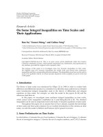
is 3 ms which gives a GP2 of 21,996 samples. As per Figure 16,
the algorithm for the RACH preamble detection can be
summarized in the following steps [45].
(1) After the cyclic prefix removal, the preprocessing
(Preproc) function isolates the RACH bandwidth, by
shifting the data in frequency and filtering it with
downsampling. It then transforms the data into the
frequency domain.
(2) Next, the circular correlation (CirCorr) function
correlates data with several prestored preamble root
sequences (or signatures) in order to discriminate
between simultaneous messages from several users. It
also applies an IFFT to return to the temporal domain
and calculates the energy of each root sequence
correlation.


EURASIP Journal on Embedded Systems
Antenna #2 to N preamble repetition #1 to P
Antenna #1 preamble repetition #2 to P
Power accumulation

Antenna #1
RACH circular correlation
Root sequence # 2 to R

Power
comp.

IFFT

Zero pad.

ZC root seq.
mult.

Subcarrier
demapping

Root sequence # 1
DFT

FIR
(bandpass filter)

Antenna #2 to N
Preamble repetition #1 to P
Antenna#1
Preamble repetition #2 to P
Antenna #1 preamble repetition #1
RACH preprocessing

Frequency shift

Antenna interface

10

Noise floor
estimation

PeakSearch

Figure 16: Random Access Channel Preamble Detection (RACH-PD) Algorithm.

(3) Then, the noisefloor threshold (NoiseFloorThr)
function collects these energies and estimates the
noise level for each root sequence.
(4) Finally, the peak search (PeakSearch) function detects
all signatures sent by the users in the current time
window. It additionally evaluates the transmission
timing advance corresponding to the approximate
user distance.

2

1
C64x+

C64x+
3

C64x+

C64x+

EDMA

EDMA

C64x+
4

C64x+
EDMA

C64x+

In general, depending on the cell size, three parameters
of RACH may be varied: the number of receive antennas,
the number of root sequences, and the number of times the
same preamble is repeated. The 115 km cell case implies 4
antennas, 64 root sequences, and 2 repetitions.
5.3. Architecture Exploration
5.3.1. Algorithm Model. The goal of this exploration is to
determine through simulation the architecture best suited
to the 115km cell RACH-PD algorithm. The RACH-PD
algorithm behavior is described as a SDF graph in PREESM.
A static deployment enables static memory allocation, so
removing the need for runtime memory administration. The
algorithm can be easily adapted to different configurations
by tuning the HSDF parameters. Using the same approach as

in [47], valid scheduling derived from the representation in
Figure 16 can be described by the compact expression:
(8Preproc)(4(64(InitPower
(2((SingleZCProc)(PowAcc))))PowAcc))
(64NoiseFloorThreshold)PeakSearch
We can separate the preamble detection algorithm in 4
steps:
(1) preprocessing step: (8Preproc),
(2) circular correlation step: (4(64(InitPower
(2((SingleZCProc)(PowAcc))))PowAcc)),
(3) noise floor threshold step: (64NoiseFloorThreshold),
(4) peak search step: PeakSearch.
Each of these steps is mapped onto the available cores
and will appear in the exploration results detailed in

C64x+

C64x+

C64x+

Figure 17: Four architectures explored.

Section 5.3.4. The given description generates 1,357 operations; this does not include the communication operations
necessary in the case of multicore architectures. Placing
these operations by hand onto the different cores would
be greatly time-consuming. As seen in Section 4.2 the
rapid prototyping PREESM tool offers automatic scheduling,
avoiding the problem of manual placement.
5.3.2. Architecture Exploration. The four architectures

explored are shown in Figure 17. The cores are all
homogeneous Texas Instrument TMS320C64x+ Digital
Signal Processors (DSP) running at 1 GHz [48]. The
connections are made via DMA links. The first architecture
is a single-core DSP such as the TMS320TCI6482. The
second architecture is dual-core, with each core similar to
that of the TMS320TCI6482. The third is a tri-core and
is equivalent to the new TMS320TCI6487 [40]. Finally,
the fourth architecture is a theoretical architecture for
exploration only, as it is a quad-core. The exploration goal
is to determine the number of cores required to run the
random RACH-PD algorithm in a 115 km cell and how to
best distribute the operations on the given cores.
5.3.3. Architecture Model. To solve the deployment problem,
each operation is assigned an experimental timing (in
terms of CPU cycles). These timings are measured with


EURASIP Journal on Embedded Systems

11

Chip

1 core

GEM 0

Real-time limit of 4 ms

3 cores
+ EDMA
4 cores
+ EDMA

GEM 1

GEM 2

C64x+
Core 0

C64x+
Core 1

C64x+
Core 2

L2 mem

2 cores
+ EDMA

L2 mem

L2 mem

Switched central resources (SCR)

Loosely timed

Approximately timed
Accurately timed

Figure 18: Timings of the RACH-PD algorithm schedule on target
architectures.

EDMA3

Inter-core
interruptions

Hardware
semaphores

DDR2 external memory

deployments of the actors on a single C64x+. Since the
C64x+ is a 32-bit fixed-point DSP core, the algorithms must
be converted from floating-point to fixed-point prior to
these deployments. The EDMA is modelled as a nonblocking
medium (see Section 4.2.2) transferring data at a constant
rate and with a given set up time. Assuming the EDMA has
the same performance from the L2 internal memory to the
L2 internal memory as the EDMA3 of the TMS320TCI6482
(see [42], then the transfer of N bytes via EDMA should
take approximately): transfer(N) = 135 + (N ÷ 3.375) cycles.
Consequently, in the PREESM model, the average data rate
used for simulation is 3.375 GBytes/s and the EDMA set up
time is 135 cycles.
5.3.4. Architecture Choice. The PREESM automatic scheduling process is applied for each architecture. The workflow

used is close to that of Figure 8. The simulation results
obtained are shown in Figure 18. The list scheduling heuristic is used with loosely-timed, approximately-timed, and
accurately-timed ABCs. Due to the 115 km cell constraints,
preamble detection must be processed in less than 4 ms.
The experimental timings were measured on code executions using a TMS320TCI6487. The timings feeding the
simulation are measured in loops, each calling a single
function with L1 cache activated. For more details about
C64x+ cache, see [48]. This represents the application
behavior when local data access is ideal and will lead to
an optimistic simulation. The RACH application is well
suited for a parallel architecture, as the addition of one core
reduces the latency dramatically. Two cores can process the
algorithm within a time frame close to the real-time deadline
with loosely and approximately timed models but high data
transfer contention and high number of transfers disqualify
it when accurately timed model is used.
The 3-core solution is clearly the best one: its CPU loads
(less than 86% with accurately-timed ABC) are satisfactory
and do not justify the use of a fourth core, as can be seen
in Figure 18. The high data contention in this case study
justifies the use of several ABC models; simple models for

Figure 19: TMS320TCI6487 architecture.

fast results and more complex models to dimension correctly
the system.
5.4. Code Generation. Developed Code libraries for the
TMS320TCI6487 and automatically generated code created
by PREESM (see Section 4.3) were used in this experiment.
Details of the code libraries and code optimizations are

given in [2]. The architecture of the TMS320TCI6487 is
shown in Figure 19. The communication between the cores
is performed by copying data with the EDMA3 from one
core local L2 memory to another core L2 memory. The cores
are synchronized using intercore interruptions. Two modes
are available for memory sharing: in symmetric mode,
each CPU has 1MByte of L2 memory while in asymmetric
mode, core-0 has 1.5 MByte, core-1 has 1 MByte and core-2
0.5 MByte.
From the PREESM generated code, the size of the
statically allocated buffers are 1.65 MBytes for one core,
1.25 MBytes for a second core, and 200 kBytes for a third
core. The asymmetric mode is chosen to fit this memory
distribution. As the necessary memory is higher than the
internal L2, some buffers are manually chosen to go in
the external memory and the L2 cache [40] is activated. A
memory minimization ABC in PREESM would help this
process, targeting some memory objectives while mapping
the actors on the cores.
Modeling the RACH-PD algorithm in PREESM while
varying the architectures (1,2,3 and 4 cores-based) enabled
the exploration of multiple solutions under the criterion
of meeting the stringent latency requirement. Once the
target architecture is chosen, PREESM can be setup to
generate a framework code for the simulated solution. As
highlighted and explained in the previous paragraph, the
statically allocated buffers by the generated code were higher
than the physical memory of the target architecture. This

12

EURASIP Journal on Embedded Systems
CPU 2

4 ms

CPU 1

Circorr32
signatures

Circorr32
signatures

Circorr32
signatures

methodologies and tools to efficiently partition code on these
architectures is thus an increasingly important objective.

CPU 0

Circorr32
signatures

Preprocess

References
Preprocess

Maximal
cadence

4 ms

4 ms

Preprocess

noiseFloor +
PeakSearch
Circorr32
signatures

Circorr32
signatures

Preprocess

Figure 20: Execution
a TMS320TCI6487.

of

the

RACH-PD

algorithm

on

necessitated moving manually some of the noncritical buffers
to external memory. This generated code, representing a
priori a good deployment solution, when executed on the
target had an average load of 78% per core while meeting
the real time deadline. Hence, the goal of decoding a RACHPD every 4 ms on the TMS320TCI6487 is thus successfully
accomplished. A simplified view of the code execution is
shown in Figure 20. The execution of the generated code had
led to a realistic assessment of a deployment very close to that
predicted with accurately timed ABC where the simulation
had shown an average load per core around 80%. These
results show that prototyping the application with PREESM
allows by simulation to assess different solutions and to give
the designer a realistic picture of the multicore solution
before solving complex mapping problems. This global result
needs to be tempered because one week-effort of manual
memory optimizations and also some manual constraints
were necessary to obtain such a fast deployment. New ABCs
computing the costs of semaphores for synchronizations
and the memory balance between the cores will reduce this
manual optimizations time.

6. Conclusions
The intent of this paper was to detail the functionalities
of a rapid prototyping framework comprising the Graphiti,
SDF4J, and PREESM tools. The main features of the framework are the generic graph editor, the graph transformation
module, the automatic static scheduler, and the code generator. With this framework, a user can describe and simulate
the deployment, choose the most suitable architecture for

the algorithm and generate an efficient framework code.
The framework has been successfully tested on RACH-PD
algorithm from the 3GPP LTE standard. The RACH-PD
algorithm with 1357 operations was deployed on a tricore
DSP and the simulation was validated by the generated code
execution. In the near future, an increasing number of CPUs
will be available in complex System on Chips. Developing

[1] E. A. Lee, “The problem with threads,” Computer, vol. 39, no.
5, pp. 33–42, 2006.
[2] M. Pelcat, S. Aridhi, and J. F. Nezan, “Optimization of
automatically generated multi-core code for the LTE RACHPD algorithm,” in Proceedings of the Conference on Design
and Architectures for Signal and Image Processing (DASIP ’08),
Bruxelles, Belgium, November 2008.
[3] J. Piat, S. S. Bhattacharyya, M. Pelcat, and M. Raulet, “Multicore code generation from interface based hierarchy,” in
Proceedings of the Conference on Design and Architectures for
Signal and Image Processing (DASIP ’09), Sophia Antipolis,
France, September 2009.
[4] M. Pelcat, P. Menuet, S. Aridhi, and J.-F. Nezan, “Scalable
compile-time scheduler for multi-core architectures,” in Proceedings of the Conference on Design and Architectures for Signal
and Image Processing (DASIP ’09), Sophia Antipolis, France,
September 2009.
[5] “Eclipse Open Source IDE,” />[6] T. Grandpierre and Y. Sorel, “From algorithm and architecture
specifications to automatic generation of distributed real-time
executives: a seamless flow of graphs transformations,” in
Proceedings of the 1st ACM and IEEE International Conference
on Formal Methods and Models for Co-Design (MEMOCODE
’03), pp. 123–132, 2003.
[7] “OpenMP,” />[8] R. D. Blumofe, C. F. Joerg, B. C. Kuszmaul, C. E. Leiserson,
K. H. Randall, and Y. Zhou, “Cilk: an efficient multithreaded

runtime system,” Journal of Parallel and Distributed Computing, vol. 37, no. 1, pp. 55–69, 1996.
[9] “OpenCL,” />[10] “The Multicore Association,” />[11] “PolyCore Software Poly-Mapper tool,” />[12] E. A. Lee, “Overview of the ptolemy project,” Technical
Memorandum UCB/ERL M01/11, University of California,
Berkeley, Calif, USA, 2001.
[13] J. Eker and J. W. Janneck, “CAL language report,” Tech.
Rep. ERL Technical Memo UCB/ERL M03/48, University of
California, Berkeley, Calif, USA, December 2003.
[14] S. S. Bhattacharyya, G. Brebner, J. Janneck, et al., “OpenDF:
a dataflow toolset for reconfigurable hardware and multicore
systems,” ACM SIGARCH Computer Architecture News, vol. 36,
no. 5, pp. 29–35, 2008.
[15] G. Karsai, J. Sztipanovits, A. Ledeczi, and T. Bapty, “Modelintegrated development of embedded software,” Proceedings of
the IEEE, vol. 91, no. 1, pp. 145–164, 2003.
[16] P. Belanovic, An open tool integration environment for efficient
design of embedded systems in wireless communications, Ph.D.
thesis, Technische Universită t Wien, Wien, Austria, 2006.
a
[17] T. Grandpierre, C. Lavarenne, and Y. Sorel, “Optimized rapid
prototyping for real-time embedded heterogeneous multiprocessors,” in Proceedings of the 7th International Workshop on
Hardware/Software Codesign (CODES ’99), pp. 74–78, 1999.
[18] C.-J. Hsu, F. Keceli, M.-Y. Ko, S. Shahparnia, and S. S.
Bhattacharyya, “DIF: an interchange format for dataflowbased design tools,” in Proceedings of the 3rd and 4th


EURASIP Journal on Embedded Systems

[19]

[20]

[21]
[22]
[23]
[24]
[25]

[26]

[27]

[28]

[29]
[30]
[31]
[32]

[33]

[34]

[35]

[36]

[37]

[38]

[39]

International Workshops on Computer Systems: Architectures,
Modeling, and Simulation (SAMOS ’04), vol. 3133 of Lecture
Notes in Computer Science, pp. 423–432, 2004.
S. Stuijk, Predictable mapping of streaming applications on multiprocessors, Ph.D. thesis, Technische Universiteit Eindhoven,
Eindhoven, The Netherlands, 2007.
B. D. Theelen, “A performance analysis tool for scenario-aware
steaming applications,” in Proceedings of the 4th International
Conference on the Quantitative Evaluation of Systems (QEST
’07), pp. 269–270, 2007.
“Graphiti Editor,” />E. A. Lee and D. G. Messerschmitt, “Synchronous data flow,”
Proceedings of the IEEE, vol. 75, no. 9, pp. 1235–1245, 1987.
“SDF4J,” />“PREESM,” />J. W. Janneck, “NL—a network language,” Tech. Rep., ASTG
Technical Memo, Programmable Solutions Group, Xilinx, July
2007.
SPIRIT Schema Working Group, “IP-XACT v1.4: a specification for XML meta-data and tool interfaces,” Tech. Rep., The
SPIRIT Consortium, March 2008.
U. Brandes, M. Eiglsperger, I. Herman, M. Himsolt, and
M. S. Marshall, “Graphml progress report, structural layer
proposal,” in Proceedings of the 9th International Symposium on
Graph Drawing (GD ’01), P. Mutzel, M. Junger, and S. Leipert,
Eds., pp. 501–512, Springer, Vienna, Austria, 2001.
J. Piat, M. Raulet, M. Pelcat, P. Mu, and O. D´ forges, “An
e
extensible framework for fast prototyping of multiprocessor
dataflow applications,” in Proceedings of the 3rd International
Design and Test Workshop (IDT ’08), pp. 215–220, Monastir,
Tunisia, December 2008.
“w3c XML standard,” />“w3c XSLT standard,” />“Grammatica parser generator,” .
J. W. Janneck and R. Esser, “A predicate-based approach

to defining visual language syntax,” in Proceedings of IEEE
Symposium on Human-Centric Computing (HCC ’01), pp. 40–
47, Stresa, Italy, 2001.
J. L. Pino, S. S. Bhattacharyya, and E. A. Lee, “A hierarchical multiprocessor scheduling framework for synchronous
dataflow graphs,” Tech. Rep., University of California, Berkeley, Calif, USA, 1995.
S. Sriram and S. S. Bhattacharyya, Embedded Multiprocessors:
Scheduling and Synchronization, CRC Press, Boca Raton, Fla,
USA, 1st edition, 2000.
V. Sarkar, Partitioning and scheduling parallel programs for
execution on multiprocessors, Ph.D. thesis, Stanford University,
Palo Alto, Calif, USA, 1987.
O. Sinnen and L. A. Sousa, “Communication contention in
task scheduling,” IEEE Transactions on Parallel and Distributed
Systems, vol. 16, no. 6, pp. 503–515, 2005.
M. R. Garey and D. S. Johnson, Computers and Intractability:
A Guide to the Theory of NP-Completeness, W. H. Freeman, San
Francisco, Calif, USA, 1990.
Y.-K. Kwok, High-performance algorithms of compiletime
scheduling of parallel processors, Ph.D. thesis, Hong Kong
University of Science and Technology, Hong Kong, 1997.
F. Ghenassia, Transaction-Level Modeling with Systemc: TLM
Concepts and Applications for Embedded Systems, Springer,
New York, NY, USA, 2006.

13
[40] “TMS320TCI6487 DSP platform, texas instrument product
bulletin (SPRT405)”.
[41] “Tms320 dsp/bios users guide (SPRU423F)”.
[42] B. Feng and R. Salman, “TMS320TCI6482 EDMA3 performance,” Technical Document SPRAAG8, Texas Instruments,
November 2006.

[43] “RapidIO,” />[44] “The 3rd Generation Partnership Project,” http://www
.3gpp.org.
[45] J. Jiang, T. Muharemovic, and P. Bertrand, “Random access
preamble detection for long term evolution wireless networks,” US patent no. 20090040918.
[46] “3GPP technical specification group radio access network;
evolved universal terrestrial radio access (EUTRA) (Release 8),
3GPP, TS36.211 (V 8.1.0)”.
[47] S. S. Bhattacharyya and E. A. Lee, “Memory management
for dataflow programming of multirate signal processing
algorithms,” IEEE Transactions on Signal Processing, vol. 42, no.
5, pp. 1190–1201, 1994.
[48] “TMS320C64x/C64x+ DSP CPU and instruction set,” Reference Guide SPRU732G, Texas Instruments, February 2008.