báo cáo hóa học:" Research Article Automatic Query Generation and Query Relevance Measurement for Unsupervised Language Model Adaptation of Speech Recognition" doc

Hindawi Publishing Corporation
EURASIP Journal on Audio, Speech, and Music Processing
Volume 2009, Article ID 140575, 12 pages
doi:10.1155/2009/140575
Research Article
Automatic Query Generation and Query Relevance
Measurement for Unsupervised Language Model Adaptation of
Speech Recognition
Akinori Ito,
1
Yasutomo Kajiura,
1
Motoyuki Suzuki,
2
and Shozo Makino
1
1
Graduate School of Engineering, Tohoku University, 6-6-05 Aramaki aza Aoba, Sendai 980-8579, Japan
2
Institute of Technology and Science, University of Tokushima 2-1, Minamijosanjima-cho, Tokushima, Tokushima 770-8506, Japan
Correspondence should be addressed to Akinori Ito,
Received 3 December 2008; Revised 20 May 2009; Accepted 25 October 2009
Recommended by Horacio Franco
We are developing a method of Web-based unsupervised language model adaptation for recognition of spoken documents. The
proposed method chooses keywords from the preliminary recognition result and retrieves Web documents using the chosen
keywords. A problem is that the selected keywords tend to contain misrecognized words. The proposed method introduces two
new ideas for avoiding the effects of keywords derived from misrecognized words. The first idea is to compose multiple queries
from selected keyword candidates so that the misrecognized words and correct words do not fall into one query. The second idea is
that the number of Web documents downloaded for each query is determined according to the “query relevance.” Combining these
two ideas, we can alleviate bad effect of misrecognized keywords by decreasing the number of downloaded Web documents from
queries that contain misrecognized keywords. Finally, we examine a method of determining the number of iterative adaptations

based on the recognition likelihood. Experiments have shown that the proposed stopping criterion can determine almost the
optimum number of iterations. In the final experiment, the word accuracy without adaptation (55.29%) was improved to 60.38%,
which was 1.13 point better than the result of the conventional unsupervised adaptation method (59.25%).
Copyright © 2009 Akinori Ito et al. This is an open access article distributed under the Creative Commons Attribution License,
which permits unrestricted use, distribution, and reproduction in any medium, provided the original work is properly cited.
1. Introduction
An n-gram model is one of the most powerful language
models (LM) for speech recognition and demonstrates high
performance when trained using a general corpus that
includes many topics. However, it is well known that an n-
gram model specialized for a specific topic outperforms a
general n-gram model when recognizing speech that belongs
to a specific topic.
An n-gram model specialized for a specific topic can
be trained by using a corpus that contains only sentences
concerning that topic, but it is time consuming, or often
impossible, to collect a huge amount of documents related
to the topic. To solve this problem, several adaptation
methods for language models have been proposed [1, 2].
The basic strategy of these methods is to exploit topic-related
documents with a general corpus. There are two major issues
with language model adaptation methods; the first is how to
calculate the adapted language model when adaptation data
are given and the second is how to gather and exploit data for
adaptation. Many methods have been proposed concerning
the first issue, including linear interpolation [3], context
dependent model combination [4], Bayesian estimation (or
maximum a posteriori estimation) [5], maximum entropy
model [6], and probabilistic latent semantic analysis [7]. The
adaptation algorithm is not the main focus of this paper; we

use adaptation based on Bayesian estimation [5, 8] in the
experiments, but other algorithms could be applied.
This paper focuses on the second issue of how to gather
the adaptation data. As mentioned before, it is costly to
gather a large amount of text data on a specific topic
manually. Two types of approach have been proposed to
overcome this problem.
Thefirsttypeofapproachusesasmallamountof
manually prepared data. Akiba et al. proposed a method for
adapting a language model using a small amount of manually
2 EURASIP Journal on Audio, Speech, and Music Processing
created sentences or examples [9]. Their method reduces
the cost of gathering the adaptation data, but is effective
only for those sentences with fixed expressions observed in
a question-answering task. Adda et al. proposed a method
that uses manually prepared text as a “seed” for selecting
adaptation data from a large text corpus [10]. In this type
of approach, a small amount of topic-related documents
is prepared first, and then similar documents are selected
from a general corpus by calculating statistical similarity
metrics such as Kullback-Leibler divergence or perplexity.
This approach assumes that sentences related to the topic
are included in the large corpus; if not, we either cannot
extract any relevant documents from the corpus, or the
extracted documents are not appropriate for the topic. One
method to overcome this problem is to use the world’s largest
collection of documents—the World Wide Web (WWW)—
as the data source. By using a Web search engine such as
Google or Yahoo, we can retrieve many documents relevant
to a specific topic using only prepared keywords concerning

the topic. Sethy et al. used linguistic data downloaded from
the WWW for building a topic-specific language model [11].
Ariki et al. used a similar method to create a language
model for transcribing sports broadcasts [12]. In addition
to specifying the query keywords manually, they can also
be chosen automatically when certain amounts of text data
representative of the topic are available [13].
The second type of approach does not use any data
prepared by humans; this kind of adaptation method is
called unsupervised language model adaptation [14, 15].
The simplest method is to use the recognized sentences as
adaptation data (self-adaptation) [15, 16],whichiseffective
when recognizing a series of recordings of a specific topic
[16]. As this framework is independent of the adaptation
algorithm, we can exploit any adaptation algorithm such
as linear interpolation [17], Bayesian estimation (count
merging) [15], or methods based on document vector space
such as LDA [18]. Iterative adaptation is also effective
[15], but the recognized sentences are often insufficient as
adaptation data, especially when the amount of speech is not
large. Niesler and Willett used the recognized sentence as the
“key” for selecting relevant sentences from a large text corpus
[14]. Bigi et al. proposed a method of using recognized
sentences as the seed text for document selection [19]. These
methods can be viewed as a combination of unsupervised
language model adaptation and adaptation text selection.
Similarly, the unsupervised language model adaptation can
be combined with the WWW. Berger and Miller [20]pro-
posed a method called “Just-In-Time language modeling.”
The Just-In-Time language model first decodes the input

speech, and then extracts keywords from the transcription.
Relevant documents are retrieved with a search engine
using the keywords. The language model is then adapted
accordingly using the downloaded data. Finally, the input
speech is decoded again using the adapted language model.
In this paper, we address the problem of obtaining
adaptation data from the WWW in an unsupervised lan-
guage adaptation manner. To implement this unsupervised
language model adaptation using the WWW, we have to
consider two issues concerning the retrieval. The first issue
is how to determine the queries to be input into a search
engine. Berger and Miller described in their paper [20] that
the queries were composed using a stop word filter, but did
not give details of the query compositions. These queries
are essential for gathering documents that are relevant to
the spoken document. As the transcribed spoken document
contains many misrecognized words, it is clear that a simple
method such as frequency-based term selection will choose
words that are not relevant to the actual topic of the spoken
document.
The second issue is how to determine the number of
queries and the number of documents to be downloaded. In
this work, we do not consider the problem of determining
the total number of documents to be downloaded, because
of the following two reasons. The first reason is that
the total number of documents for downloading depends
on the adaptation method, the general corpus and the
task. The second reason is that the total number is also
restricted by the processing time required, as the time taken
to download documents is roughly proportional to the

number of documents. Therefore, if we have a limitation
on processing time, the number of downloaded documents
is limited accordingly. Therefore, we assume that the total
number of documents is determined empirically.
On the other hand, if we use more than one query for
downloading documents, we have to decide the number
of documents to be downloaded by each query even if we
fix the total number of documents. Generally speaking, the
quality of downloaded documents in terms of adaptation
performance differs from query to query, so we want to
download more documents from “good” queries. In our
previous work [21], we composed multiple queries, each
of which had a single keyword. Within that framework, we
retrieved an equal number of documents for each query,
but this proved to be problematic because some queries
contained keywords derived from misrecognitions.
In this paper, we propose a method of query composition
and document downloading for adaptation of language
model of a speech recognizer, based on Web data using
a search engine. The framework of the adaptation is
similar to the Just-In-Time language model, but with the
following three differences. The first is the method with
which the queries are composed in order to search for
relevant documents with a Web search engine. The second
is how the number of documents to be downloaded for
each query is determined. The adaptation method is also
different. Berger and Miller used a maximum-entropy-based
adaptation method, whereas our method is based on an n-
gram count mixture [5, 8, 15]. However, this difference only
concerns implementation and is not essential for using our

query composition method.
Note that an adaptation based on this framework takes a
great amount of time for generating the final transcription,
becausewehavetorecognizethespeechdocumentat
least twice, download thousands of Web documents, and
train a language model. Therefore, this kind of method is
not suitable for real-time speech transcription, but can be
used for off-line transcription tasks such as transcribing a
recording of a lecture.
EURASIP Journal on Audio, Speech, and Music Processing 3
General
corpus
Te x t f o r
adaptation
General
n-gram
We b se arc h
engine
First
transcription
Recognition
result
Spoken
document
Query
generation
Decoder
Queries
URLs
Downloader

Te x t
filter
Decoder
Adapted
n-gram
Iterative
adaptation
Query
relevance
measurement
Wor ld Wi de We b
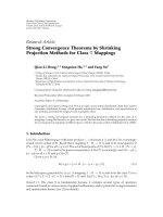
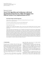
Figure 1: Overview of the proposed system.
2. Unsupervised Language Model Adaptation
Using a Web Search Engine
2.1. Basic Framework. In this section, we introduce the basic
framework of the unsupervised language model adaptation
using a Web search engine [20], and evaluate its performance
as a baseline result. Figure 1 shows the basic framework of
the adaptation. First, we train a baseline language model
(thegeneraln-gram)fromalargegeneralcorpussuchasa
newspaper corpus. Then a spoken document is automatically
transcribed using a speech recognizer with the general n-
gram to generate the first transcription. Several keywords
are selected from the transcription, and those keywords are
used as a query given to the Web search engine. URLs
relevant to the query are then retrieved from the search
results. HTML documents denoted by the retrieved URLs
are then downloaded, and are formatted using a text filter.
The formatted sentences are used as text for adaptation,
and the adapted n-gram is trained. The spoken document

is then recognized again using the adapted n-gram. This
process may be iterated several times [15] to obtain further
improvement.
2.2. Implementation of the Baseline System. We implemented
the speech recognition system with the unsupervised LM
adaptation. Note that the details of the investigated method
here are slightly different from those of the conventional
method [20], but these differences are only a matter of
implementation and do not constitute the novel aspects of
this paper (therefore the results in this section are denoted as
“Conventional”).
We used transcriptions of 3,124 lectures (containing
about 7 million words) as a general corpus taken from the
Corpus of Spontaneous Japanese (CSJ) [22]. The language
model for generating the first transcription is a back-off
trigram with 56,906 lexical entries, which are all words that
appear in the general corpus. The baseline vocabulary for
the adaptation has 39,863 lexical entries that appear more
than once in the general corpus. The most frequent words
in the downloaded text are added to the vocabulary, and the
vocabulary size grows to 65,535. The reason why we used
different vocabularies for generating the first transcription
and the baseline vocabulary for adaptation was that the
upper limit of the vocabulary size for the decoder was
65,535. If we were to use a baseline vocabulary of more than
56,000 words, we could add fewer than 10,000 words in the
adaptation process. Conversely, we could reserve space for
more additional vocabulary by limiting the size of the first
vocabulary.
Julius version 3.4.2 [23] was used as a decoder, with

the gender-independent 3,000-state phonetic tied mixture
HMM [24] as an acoustic model. The keywords were selected
from the transcription based on tf
·idf. On calculating
tf
·idf values, the term frequencies were calculated from the
transcription. In addition, two years’ worth of articles from
a Japanese newspaper (Mainichi Shimbun) were added to
the general corpus for the calculation of idf. There were
208,693 articles in the newspaper database, which contained
about80millionwords.Thesegeneralcorporaaswellas
the downloaded Web documents were tokenized by the
morphemic analyzer ChaSen [25]. Morphemic analysis is
indispensable for training a language model for Japanese
because Japanese sentences do not have any spaces between
words and so sentences must be split into words using a
morphemic analyzer before training a language model. Using
a morphemic analyzer, we also can obtain pronunciations of
words.
The Web search is performed on the Yahoo! Japan
Website, using the Yahoo API [26]. As the Yahoo API
4 EURASIP Journal on Audio, Speech, and Music Processing
returns a maximum of 1,000 URLs as search results, when
more documents are needed the system performs recursive
download of Web documents by following links contained
in the already downloaded documents. When downloading
Web documents, there is a possibility of downloading one
document more than once, since the same document could
be denoted by multiple URLs. However, we do not perform
any special treatment for such documents downloaded

multiple times because it is not easy to completely avoid
duplicate downloading.
Collected Web documents are input into a text filter
[27]. The filter excludes Web documents written in other
than the target language (Japanese in this case). The filtering
is performed in three stages. In the first stage, HTML
tags and JavaScript codes are removed based on a simple
pattern matching. In the second stage, the document is
organized into sentence-like units based on punctuation
marks, and then the units that contain more than 50%
US-ASCII characters are removed because those units are
likely to be other than Japanese sentences. Finally, character-
based perplexities are calculated for every unit, based on
a character bigram trained from 3,128 lectures in the
Corpus of Spontaneous Japanese [22].Theunitswhose
character perplexity values are higher than a threshold are
removed from the training data because those units with
high perplexity values are considered to be other than
Japanese (which could be Chinese, Korean, Russian or any
other language coded by other than US-ASCII). A perplexity
threshold of 200 was used in [27], but we used a threshold
of 800 because it showed a lower out-of-vocabulary (OOV)
rate in a preliminary experiment. After selecting the text
data, each sentence in the data is split into words using the
morphemic analyzer.
Next, a mixed corpus is constructed by merging the
general corpus and the extracted sentences, and the adapted
n-gram model is trained by the mixed corpus [8]. Of course,
we could have used other adaptation methods such as linear
interpolation or adaptation based on the maximum entropy

framework; the reason why we chose the simple corpus
mixture (which is equivalent to the n-gram count merge)
is that we can easily use the adapted language model with
the existing decoder because the adapted n-gram by corpus
mixture is simply an ordinary n-gram.
We did not weigh the n-gram count of the downloaded
text for mixing the corpora. Using an optimum weight, we
can improve the accuracy. However, we did not optimize the
weight for two reasons. First, it was difficult to determine the
optimum weight automatically, because we employed an n-
gram count merge, for which determination of the optimum
weight should be performed empirically. Second, the pre-
liminary experiments suggested that the recognition results
without optimization of weight were not very different from
those that did use the optimally determined weights.
2.3. Experimental Conditions. We used 10 lectures (contain-
ing about 18,000 words) for evaluation, which are included
in the CSJ and are not included in the training corpus. These
lectures are taken from the section “Objective explanations
Table 1: Lectures for evaluation.
ID ID in CSJ Title No. of words
0 S04M0609 History of character 1420
1 S04M1191 Lottery 1285
2 S04M1552 Paintings in America and Europe 1092
3 S04F0496 Effect of charcoal 2330
4 S04F1497 Accounting work 1478
5 S04F0925 Brushing teeth 1957
6 S04F1417 Golden retriever 2184
7 S04M0794 Miscellaneology 1407
8 S04M0618 The reason why I was fired 2415

9 S04M1569 The steel industry 2202
Total 17770
of what you know well or you are interested in” in the
CSJ. The topics of the chosen 10 lectures were independent
from those of other lectures in the CSJ. The IDs and titles
of the lectures are shown in Ta bl e 1. The total number of
downloaded documents was set to 1,000, 2,000 or 5,000.
2.4. Experimental Results. Figure 2 shows the experimental
result when the adaptation was performed only once. In
this figure, “top-1” denotes the result when we used only
one keyword with the highest tf
·idf as a query, while “top-
2” denotes the result when two keywords were used as a
query, which was determined as the best number of keywords
from the preliminary experiment on the same training and
test set. This result clearly shows that the unsupervised LM
adaptation using Web search is effective.
Figure 3 shows the effect of iterative adaptation. In this
result, the top-2 keywords are used for downloading 2,000
documents. Iterative adaptation is effective, and we can
obtain an improvement of around 2.5 points by iterating
the adaptation process compared to the result of the first
adaptation.
2.5. Problems of the Conventional Method. Although the
conventional LM adaptation framework is effective for
improving word accuracy, it has a problem; those words
derived from misrecognition are mixed among the selected
keywords. Table 2 shows the selected keywords of the test
documents when two keywords were selected at the first
iteration. The italicized words denote the words derived from

misrecognition. From this result, three out of ten queries
contain misrecognized words. Figure 4 shows the average
absolute improvement of word accuracy for documents with
misrecognized queries (ID 0, 3, 7) and without them (ID 1,
2, 4, 5, 6, 8, 9) at the first iteration with respect to the number
of downloaded documents. We can see that the improvement
of accuracy for documents with misrecognized queries is
smaller than that for other documents, indicating that we
need to develop a method for avoiding using misrecognized
wordsasaquery.
EURASIP Journal on Audio, Speech, and Music Processing 5
Number of retrieved web documents
0 1000 2000 3000 4000 5000 6000
Word accuracy (%)
55
55.5
56
56.5
57
57.5
58
58.5
To p - 1
To p - 2
Figure 2: Word accuracies by the adaptation (no iteration).
0123456
Iteration
55
55.5
56

56.5
57
57.5
58
58.5
59
95.5
60
Word accuracy (%)
Figure 3: Word accuracies by the adaptation (effect of iterative
adaptation).
0
0.5
1
1.5
2
2.5
3
Word accuracy improvement (pt)
0 1000 2000 3000 4000 5000
Number of retrieved web documents
With misrecognition
Without misrecognition
Figure 4: Word accuracy improvement for queries with or without
misrecognized words.
Table 2: Selected keywords (top 2).
3. Query Composition and Determination of
Number of Downloaded Documents
3.1. Concept. From the observation of the previous section,
we need to develop a method for avoiding using misrec-

ognized words in a query. However, it is quite difficult
to determine whether a recognized word is derived from
misrecognition. A straightforward way of determining the
correctness of a word is to exploit a confidence measure,
which is calculated from the acoustic and linguistic scores
of recognition candidates. However, the acoustic confidence
measure does not seem to be helpful in this case. For
example, the misrecognized keyword
(household) in
document ID 0 is pronounced as /shotai/, which is a
homonym of the correct keyword
(font). Therefore, it
is impossible to distinguish these two keywords acoustically.
Besides, as the baseline language model is not tuned to a
specific topic, it is also difficult to determine that “font” is
more likely than “household.”
To solve this problem, we combined two ideas. One
idea is to cluster the selected keyword candidates so that
the misrecognized words do not fall into the same cluster
that contains correct words. Each of the resulting clusters
is used as an independent query. The other idea is to
estimate how relevant a query is to the spoken document
to be transcribed. If a query is not relevant to the spoken
document, we just abandon it. By combining these two ideas,
we can exclude the unrelated adaptation data caused by the
misrecognized words. It may seem difficult to measure the
relevance of a query for the same reason it is difficult to
determine misrecognized words. The principle is that we
do not measure the relevance of words in a query directly;
instead, we measure the relevance of downloaded documents

using the query. This makes sense because what we need for
LM adaptation is not a query but downloaded documents.
6 EURASIP Journal on Audio, Speech, and Music Processing
To realize the first idea, we propose a keyword clustering
algorithm based on word similarity. For the second idea, we
propose a method to measure the relevance of a query using
document vector.
3.2. Keyword Clustering Algorithm Based on Word Similarity.
To create keyword clusters, we first select keyword candidates
from the first transcription of the spoken document, and
then the keyword candidates are clustered.
Word clustering techniques are widely used in the
information retrieval (IR) field. However, most works in IR
use word clustering for word sense disambiguation [28]and
text classification [29, 30]. Boley et al. used word clustering
for composing a query [31], but the purpose of word
clustering in their work was to choose query terms, which
is different from our work, and in fact, they used only one
query for relevant document retrieval.
The keyword candidates are selected from nouns in the
transcription generated by the first recognition. The keyword
selection is based on keyword score [21]. It is basically a
tf
·idf score, where the tf is calculated from the transcription
and the idf is calculated from the general corpus. We use
the top 10 words with highest tf
·idf values as keyword
candidates in the later experiments. We could use a variable
number of words based on tf
·idf score, but we decided to

use a fixed number of candidates because we would have
to control the number of candidates so that a sufficient
number of candidates was obtained when variable numbers
of candidates were used.
Next, we cluster the keyword candidates based on word
similarity. If we can define similarity (or distance) between
any two keyword candidates, we can exploit an agglomerative
clustering algorithm. We therefore defined word similarity
based on the document frequency of a word in the WWW
obtained using a Web search engine. Let us consider the
number of Web documents retrieved using two keywords.
If two keywords belong to the same topic, the number of
documents should be large. Conversely, the number of doc-
uments should be small if the two keywords are unrelated.
Following this assumption, we define the similarity between
two keywords as the number of retrieved Web documents.
Let d(w) be the number of Web documents that contain
awordw,andd(w
1
, w
2
) be the number of documents that
contain both words w
1
and w
2
. The numbers of documents
are obtained using the Yahoo API. The similarity between the
two words sim(w
1

, w
2
) is then calculated as follows:
sim
(
w
1
, w
2
)
=
2d
(
w
1
, w
2
)
d
(
w
1
)
+ d
(
w
2
)
. (1)
This definition is the same as the Dice coefficient [32].

Now we can perform an agglomerative clustering for the
set of keywords. Initially, all keywords belong to their own
singleton clusters. Then the two clusters with the highest
similarity are merged into one cluster. The new similarity
between clusters C
1
and C
2
is defined as equation (2). This
definition of similarity corresponds to the furthest-neighbor
A
{A}
{A, B}
{A, B, C}
{A, B, C, D}
Root node
{A, B, C, D, E, F}
B
C
D
E
F
{B}
{C}
{D}
{E}
{F}
{E, F}
Figure 5: An example of a tree generated by the keyword clustering.
method of an ordinary clustering using the distance between

two points,
sim
(
C
1
, C
2
)
= min
w∈C
1
,v∈C
2
sim
(
w, v
)
. (2)
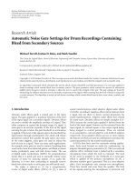
This clustering method generates a tree as shown in Figure 5.
In this example, A, B, , F are keywords, and a node in the
tree corresponds to a cluster of keywords. The root node
of the tree corresponds to a cluster that contains all of the
keywords.
After clustering, clusters corresponding to queries are
extracted.Ingeneral,whenweusemorekeywordsinan
AND query, the number of retrievable documents (i.e.,
number of Web documents that contains all keywords in
the query) become smaller, and vice versa. If the number
of retrievable documents is too large, it means that the
query is underspecified, and the retrieved documents are

not expected to have the same topic as that of the given
spoken document. Conversely, if the number of retrievable
documents is too small, we cannot gather sufficient number
of Web documents for the adaptation. Therefore, given
anumberofWebdocumentsn
θ
, the objective of query
composition here is to find clusters so that
(1) each of the clusters contain keywords with which
more than n
θ
documents are retrieved,
(2) if any nearest two clusters in the determined clusters
are merged, the number of retrievable Web docu-
ments using the keywords in the merged cluster is less
than n
θ
.
Next, we explain an algorithm for finding the clusters. Let
d(n) be the number of Web documents that can be retrieved
using a query composed by the keywords in a node n in the
tree. For example, if n is the root node of the tree in Figure 5,
d(n) is the number of Web documents retrieved by the AND
query composed by the six keywords, A, B, C, D, E and F.
This number can be obtained from a Web search engine.
Note that Yahoo! API returns the number of documents even
when the number is more than 1,000, though the maximum
number of actually retrievable URLs is 1,000. The limit of
EURASIP Journal on Audio, Speech, and Music Processing 7
Q ←∅, S ←∅

Add the root node to Q
while Q is not empty
for all node n in Q
Remove n from Q
if d(n) >n
θ
then
Add n to S
else if n has no child nodes, then
Add n to S
else
Add all child nodes of n to Q
end if
end for
end while
return S
Algorithm 1: An algorithm for determination of queries.
retrievable URLs is not a problem here because we only
need the number of documents for the clustering. Then, we
determine the threshold n
θ
that is the minimum number of
Web documents retrieved by the query. Let Q and S be the
set of “current nodes under search” and “selected nodes,”
respectively. We then use Algorithm 1 for determining the
number of queries and keywords that correspond to the
queries.
All keywords that correspond to a node in S are used
as a single query. Then Web documents are retrieved using
each query, and all the retrieved Web documents are used for

adaptation.
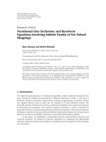
An example of the clustering result and selected keywords
are shown in Figure 6. In this figure, black nodes in the
tree denote the “selected nodes.” There are six keyword
candidates (word “A” to “F”), and three clusters are selected.
Retrieval of Web documents is carried out three times using
the keywords in queries 1, 2 and 3.
A misrecognized word belongs to a different topic from
the correct words. As a result, a misrecognized word is
separated from the correct words.
We carried out an experiment to cluster the keyword
candidates for the 10 test documents, using the experimental
conditions described in Section 2.3.
First, a selected keyword list was investigated. We chose
10 keyword candidates for the 10 documents making
100 words in total. Among them, 23% of the keywords
were misrecognized words. After the clustering, 48 queries
are generated (4.8 queries/document). Among them, 29
queries (60.4%) contain only correctly recognized words,
15 queries (31.2%) contain only misrecognized words
and the remaining 4 queries (8.3%) contain both correct
and misrecognized words. This result shows that most of
the misrecognized words could be separated from correct
words. The average number of words in a query with only
correctly recognized words was 2.10, while that with only
misrecognized words was 1.07. This result indicates that a
misrecognized word tend to be classified into a singleton
cluster.
A
{A}

{A, B}
{A, B, C}
{A, B, C, D}
Root node
{A, B, C, D, E, F}
B
C
D
E
F
{B}
{C}
{D}
{E}
{F}
{E, F}
Query 1
Query 2
Query 3
A and B and C
D
EandF
Figure 6: An example of hierarchical clustering and selected key-
words.
Table 3: Examples of selected keywords and clusters.
(a) Results for the document “History of characters (ID 0).”
(b) Results for the document “Paintings in America and Europe (ID 2).”
Ta bl e 3 shows the selected keywords and clusters from
two lectures on “History of characters” (ID 0) and “Paintings
in America and Europe” (ID 2). In this table, italicized words

denote the misrecognitions. Both examples illustrate how
appropriate clusters were acquired and most misrecognitions
were separated from the correct words.
8 EURASIP Journal on Audio, Speech, and Music Processing
3.3. Estimation of the Optimum Number of Downloaded
Documents. Next, we explain a method to measure the
relevance of a query to the spoken document. We call
this metric “query relevance.” After estimating the query
relevance of a query, we use that value for determining the
number of documents to be downloaded using that query.
As explained before, if a query is not relevant to the spoken
document, we do not use that query. However, a binary
classification of a query into “relevant” or “not relevant”
is difficult. Therefore, we use a “fuzzier” way of using the
query relevance: we determine the number of downloaded
documents by a query so that the number is proportional to
the value of query relevance.
In the proposed method, a small number (up to 100
documents) of documents are downloaded for each of the
composed queries. Then the relevance of the downloaded
text to the spoken document is measured. The query
relevance is a cosine similarity between the first transcription
and the downloaded text.
Let I be the number of nouns in the vocabulary, v
i
be
the tf
·idf score of the ith noun in the first transcription, and
w
i,j

be that of the ith noun in the downloaded text by the jth
query. Word vectors v and w
j
are
v
=
(
v
1
, , v
I
)
w
j
=

w
1,j
, , w
I, j

.
(3)
The query relevance of the jth query is calculated as
Q
j
=
v · w
j
|v|




w
j



. (4)
This value roughly reflects the similarity of unigram distri-
bution between the transcription and a downloaded text.
If the two distributions are completely identical, this value
becomes 1. Conversely, if the distributions are different, the
value becomes smaller. Thus, if a query has a high query
relevance value, it can be said that the query retrieves Web
documents with similar topics to the transcription of the
spoken document.
In addition to the above calculation, the threshold Q
th
is
introduced to prune queries that have low query relevance:
Q

j
=
⎧
⎨
⎩
Q
j

if Q
j
>Q
th
,
0 otherwise.
(5)
The number of downloaded documents using the jth
query is calculated as follows. First, the total number of
downloaded documents N
d
is determined. This number is
determined empirically, and our previous work suggests that
5,000 documents are enough [21]. Let N
q
be the number of
all queries. Then, the number of documents downloaded by
the jth query is proportional to the query relevance of the jth
query, calculated as
N
j
= N
d
·
Q

j

N
q

k=1
Q

k
. (6)
0
0.1
0.2
0.3
0.4
0.5
0.6
0 20 40 60 80 100 120 140
Correlation coefficient
Number of downloaded web document
Figure 7: Number of downloaded documents n
p
and correlation
coefficient.
Note that the number of downloaded documents for
measurement of the query relevance is included in N
j
.
For example, if we use 100 documents for measuring the
query relevance, the number of additionally downloaded
documents by the jth query will be N
j
−100.
3.4. Evaluation of Query Relevance. To evaluate the reliability
of the query relevance, we first measured query relevance val-

ues for queries composed in the previous experiment based
on n
p
documents of downloaded text. Next, we performed
speech recognition experiments for each of the queries using
a language model adapted by using 1,000 documents of
downloaded text from the query. Then the improvement
of word accuracy from the baseline was calculated. Finally,
we examined the correlation coefficients between the query
relevances and the accuracy improvements. If they are
correlated, we can use the query relevance as an index of
improvement of the language model.
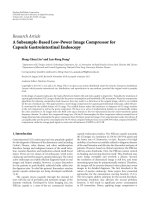
Figure 7 shows the relationship between n
p
and the
correlation coefficient. Correlation coefficient values in this
graph are the averages for the 10 test documents used for
the experiment. Q
th
was set to 0. This result shows that we
obtain a correlation of more than 0.5 by using more than 50
documents. We used 100 documents in the later experiments
for estimating the query relevance.
Figure 8 shows the correlation coefficients for all docu-
ments when using 100 documents for estimating the query
relevance. In this figure, both the Q
th
= 0 case and the
optimum Q
th

case are shown. We estimated the optimum Q
th
using 10-fold cross validation for each document. Note that
the cross validation was performed on the test set; therefore,
this result is the “ideal” result. The estimated values of Q
th
were 0.09 for document ID 8, 0.14 for ID 9 and 0.12 for
all of the other documents. In the test document ID 3, 7
and 8, the correlations using the optimum Q
th
were smaller
than those when Q
th
= 0. In these documents, the queries
with high query relevance did not necessarily gather relevant
Web documents. Especially, queries that contain both correct
and misrecognized words were included in the queries of
EURASIP Journal on Audio, Speech, and Music Processing 9
Correlation coefficient
−0.8
−0.6
−0.4
−0.2
0
0.2
0.4
0.6
0.8
1
ID 0 ID 1 ID 2 ID 3 ID 4 ID 5

ID 6 ID 7 ID 8
ID 9 Ave
Q
th
= 0
Optimum Q
th
Figure 8: Correlation coefficient for each document.
0 1000 2000 3000 4000 5000
55
55.5
56
56.5
57
57.5
58
58.5
59
Word accuracy (%)
Number of retrieved web documents
Conventional
Proposed
Figure 9: Comparison of word accuracy by the conventional and
proposed methods.
ID 7 and 8, which had not very small query relevance values
(1.4 for ID 7, 22.7 for ID 8). This fact seems to be a reason
why we could not determine the optimum threshold of query
relevance.
This result shows that we can obtain a correlation coef-
ficient of 0.55 between the query relevance and the accuracy

improvement, on average. In addition, we can improve the
correlation using an optimum threshold.
4. Evaluation Experiment
4.1. Effect of the Proposed Query Composition and Determina-
tion of Number of Documents. We conducted an experiment
for evaluating the proposed method. First, we investigated
whether the proposed method (keyword clustering and
estimation of query relevance) solved the problem shown in
Figure 4. In this experiment, the adaptation was performed
only once; iteration was not performed. The threshold n
θ
was
set to 30,000 and n
p
was set to 100.
0
0.5
1
1.5
2
2.5
3
3.5
4
4.5
5
0 1000 2000 3000 4000 5000
Word accuracy improvement (pt)
Number of retrieved web documents
With misrecognition

Without recognition
Figure 10: Word accuracy improvement using the proposed
method.
Figure 9 shows the word accuracy by the conventional
and proposed methods. In this result, the proposed method
gave slightly better word accuracy. We conducted two-way
layout ANOVA to compare the result of the conventional
and proposed methods, excluding the no adaptation case
(number of retrieved documents
= 0). As a result, the
difference of the methods (conventional/proposed) was
statistically significant (P
= .0324) while the difference of
the number of retrieved documents was not significant (P
=
.0924).
Figure 10 shows the word accuracy improvement, cal-
culated for two groups of documents (ID 0, 3, 7 as “with
misrecognition” group, and all other documents as “without
misrecognition” group). This figure can be compared with
Figure 4. From the comparison between Figures 4 and 9,it
is found that the performance for the “without misrecogni-
tion” group is almost the same in the two results, while that
for the “with misrecognition” group was greatly improved
by the proposed method. We conducted two-way layout
ANOVA for “with misrecognition” results of Figures 4 and
9 (excluding no adaptation case, where number of retrieved
Web documents was 0). As a result, method (conventional
=
Figure 4, proposed

=
Figure 9) was significant (P
=
.0004) and the number of retrieved Web documents was
also significant (P
= .0091). This result proves that the
proposed method effectively avoided the harmful influence
of misrecognized words in queries.
4.2. Effect of Iteration. Next, we conducted an experiment
with iterative adaptation. In this experiment, 2,000 docu-
ments were used for adaptation at each of the iterations.
Figure 11 shows the word accuracy result with respect to the
number of iteration. From this result, the proposed method
gave better performance than the conventional method.
We conducted two-way layout ANOVA (excluding the no
adaptation case where the number of iterations was 0). As
a result, the difference of methods (proposed/conventional)
was statistically significant (P
= .0003) and the difference of
10 EURASIP Journal on Audio, Speech, and Music Processing
55
56
57
58
59
60
61
0123456
Conventional
Proposed

Word accuracy (%)
Number of iterations
Figure 11: Result of iterative adaptation.
55
57
59
61
63
65
67
69
0123456
ID 0
ID 8
Word accuracy (%)
Number of iterations
Figure 12: Word accuracy at each number of iterations.
iteration count was also significant (P = .0002). From this
result, the proposed method was proved to be also effective
when iterative adaptation was performed.
5. Iterative Adaptation a nd
the Stopping Criterion
5.1. Problem of Iterative Adaptation. As explained in Sections
2 and 4, iterative adaptation is effective for improving
word accuracy. However, there are still two problems. First,
we want to reduce the number of iterations because the
adaptation procedure using WWW is slow. If we can cut the
number of iterations in half, the adaptation procedure will
be almost two times faster. Second, the optimum number
of iterations varies from document to document. Word

accuracy does not necessarily converge when we iterate the
adaptation process. Figure 12 shows the number of iterations
and word accuracy for two of the test documents. While
0
0.5
1
1.5
2
2.5
3
3.5
4
4.5
5
OOV rate (%)
Number of iterations
0123456
ID 0
ID 8
Figure 13:OOVrateateachnumberofiterations.
Recognize D, and generate R
0
and L
0
k ← 1
loop forever
Perform adaptation using the transcription R
k−1
Recognize D, and generate R
k

and L
k
if L
k
≤ L
k−1
then
R
k−1
becomes the final recognition result
stop
end if
k
← k +1
end loop
Algorithm 2: The adaptation procedure with iteration.
the accuracy of document ID 0 converges, the accuracy
of document ID 8 begins to degrade when the adaptation
process is iterated two or more times. Figure 13 shows
the OOV rate of the two documents for each number of
iterations. The OOV rate of document ID 0 decreases until
the third iteration, whereas the OOV rate of document ID
8 slightly increases at the first iteration and does not change
at all from the following iteration. These examples illustrate
the need to introduce a stopping criterion to find the best
number of iterations document by document.
5.2. Iteration Stopping Criterion Using Recognition Likelihood.
We examined a simple way of determining whether or not
the iteration improves the recognition performance using
recognition likelihood. This method monitors the recogni-

tion likelihood every time we recognize the speech, and stops
the iteration when the likelihood begins to decrease. Let R
k
be the recognition result (a sequence of words) of the spoken
document D after k iterations of adaptation. Let L
k
be the
total likelihood of R
k
. The adaptation procedure is as shown
in Algorithm 2.
EURASIP Journal on Audio, Speech, and Music Processing 11
55
55.5
56
56.5
57
57.5
58
58.5
59
59.5
60
60.5
61
Word accuracy (%)
Number of iterations
0123456
Conventional (fixed)
Proposed (fixed)

Conventional (auto)
Proposed (auto)
Proposed (oracle)
Figure 14: Experimental result of iteration number determination.
Table 4: Number of iterations.
ID Conventional method Proposed method
Likelihood Oracle
ID 0 4 + 1 5 + 1 5
ID 1 3 + 1 2 + 1 2
ID 2 2 + 1 2 + 1 2
ID 3 1 + 1 5 + 1 5
ID 4 3 + 1 3 + 1 5
ID 5 3 + 1 2 + 1 2
ID 6 1 + 1 1 + 1 4
ID 7 4 + 1 5 + 1 5
ID 8 1 + 1 1 + 1 1
ID 9 1 + 1 1 + 1 0
Ave 3.3 3.7 3.1
5.3. Experimental Results. We carried out experiments
to investigate the effectiveness of the proposed itera-
tion method, using the same experimental conditions as
described in the previous section.
The results are shown in Figure 14. In this figure,
“Conventional (fixed)” and “Proposed (fixed)” are the same
results as shown in Figure 11.“Conventional(auto)”and
“Proposed (auto)” are the results where the proposed stop-
ping criterion was used for the conventional and proposed
adaptation methods, respectively. “Proposed (oracle)” is the
result when using the proposed method for adaptation and
the number of iterations was determined document by

document a posteriori so that the highest word accuracy
was obtained. Note that the number of iterations of the
“auto” conditions is the average of the determined number of
iterations. As explained above, we need to carry out one more
adaptation to confirm that the current iteration number is
optimum.
As shown in Figure 14, we could reduce the number of
iterations while maintaining high word accuracy. When the
proposed adaptation method was used, the result using the
proposed stopping criterion was better than any result using
a fixed number of iterations. Moreover, the result obtained
by the proposed method was only 0.23 points behind the
optimum result (oracle), which shows that the proposed
stopping criterion was almost the best.
Ta bl e 4 shows the determined number of iterations when
the likelihood-based stopping criterion was used. Numbers
such as “5 + 1” mean that adaptation was performed six
times and recognition results from the fifth adaptation were
determined as the final recognition result. This result shows
that we can determine the optimum number of iterations for
7 out of 10 documents.
6. Conclusion
In this paper, we proposed a new method for gathering
adaptation data using the WWW for unsupervised language
model adaptation. Through an experiment of conventional
unsupervised LM adaptation using Web documents, we
found a problem that misrecognized words are selected
as keywords for Web queries. To solve this problem, we
proposed a new framework for gathering Web documents.
First, the selected keyword candidates are clustered so that

correct and misrecognized words do not fall into the same
cluster. Second, we estimated the relevance of a query to the
spoken document using the downloaded text. The estimated
relevance values were then used for determining the number
of Web documents to be downloaded.
Experimental results showed that the proposed method
yielded significant improvements over the conventional
method. Especially, we obtained a bigger improvement for
documents with misrecognized keyword candidates.
Next, we proposed a method for automatically determin-
ing the number of iterative adaptations based on recognition
likelihood. Using the proposed method, we could reduce the
number of iterations while maintaining high word accuracy.
Some parameters in this system are given apriori.For
example, the number of keyword candidates or threshold of
query composition is determined by a limited number of
preliminary experiments. As a future work, we are going to
investigate the effect of these parameters and find the best
way to determine the parameters.
References
[1] R. Rosenfeld, “Two decades of statistical language modeling:
wheredowegofromhere?”Proceedings of the IEEE , vol. 88,
no. 8, pp. 1270–1278, 2000.
[2] J. R. Bellegarda, “Statistical language model adaptation: review
and perspectives,” Speech Communication,vol.42,no.1,pp.
93–108, 2004.
[3] R. Iyer and M. Ostendorf, “Modeling long distance depen-
dence in language: topic mixtures vs. dynamic cache models,”
IEEE Transactions on Speech and Audio Processing, vol. 7, no. 1,
pp. 30–39, 1996.

[4] X. Liu, M. J. F. Gales, and P. C. Woodland, “Context dependent
language model adaptation,” in Proceedings of the International
Speech Communicatiuon Association (Interspeech ’08), pp. 837–
840, Brisbane, Australia, September 2008.
12 EURASIP Journal on Audio, Speech, and Music Processing
[5] M. Federico, “Bayesian estimation methods for n-gram lan-
guage model adaptation,” in Proceedings of the International
Conference on Spoken Language Processing (ICSLP ’96), vol. 1,
pp. 240–243, Philadelphia, Pa, USA, October 1996.
[6] R. Rosenfeld, “A maximum entropy approach to adaptive sta-
tistical language modelling,” Computer Speech and Language,
vol. 10, no. 3, pp. 187–226, 1996.
[7] T. Hofmann, “Unsupervised learning by probabilistic latent
semantic analysis,” Machine Learning, vol. 42, no. 1-2, pp. 177–
196, 2001.
[8] A. Ito, H. Saitoh, M. Katoh, and M. Kohda, “N-gram language
model adaptation using small corpus for spoken dialog
recognition,” in Proceedings of the 5th European Conference on
Speech Communication and Technology (Eurospeech ’97),pp.
2735–2738, Rhodes, Greece, September 1997.
[9] T. Akiba, K. Itou, and A. Fuji, “Language model adaptation
for fixed phrases by amplifying partial N-gram sequences,”
Systems and Computers in Japan, vol. 38, no. 4, pp. 63–73,
2007.
[10] G. Adda, M. Jardino, and J. L. Gauvain, “Language modeling
for broadcast news transcription,” in Proceedings of the
European Conference on Speech Communication and Tech-
nology (Eurospeech ’99), pp. 1759–1762, Budapest, Hungary,
September 1999.
[11] A. Sethy, P. G. Georgiou, and S. Narayanan, “Building topic

specific language models from webdata using competitive
models,” in Proceedings of the 9th European Conference on
Speech Communication and Technology (Eurospeech ’05),pp.
1293–1296, Lisbon, Portugal, September 2005.
[12] Y. Ariki, T. Shigemori, T. Kaneko, J. Ogata, and M. Fujimoto,
“Live speech recognition in sports games by adaptation of
acoustic model and language model,” in Proceedings of the
8th European Conference on Speech Communication and Tech-
nology (Eurospeech ’03), pp. 1453–1456, Geneva, Switzerland,
2003.
[13]T.Ng,M.Ostendorf,M Y.Hwang,M.Siu,I.Bulyko,and
X. Lei, “Web-data augmented language models for mandarin
conversational speech recognition,” in Proceedings of the
IEEE International Conference on Acoustics, Speech and Signal
Processing (ICASSP ’05), vol. 1, pp. 589–592, Philadelphia, Pa,
USA, March 2005.
[14] T. Niesler and D. Willett, “Unsupervised language model
adaptation for lecture speech transcription,” in Proceedings of
the 7th International Conference on Spoken Language Processing
(ICSLP ’02), pp. 1413–1416, Denver, Colo, USA, September
2002.
[15] M. Bacchiani and B. Roark, “Unsupervised language model
adaptation,” in Proceedings of the IEEE International Confer-
ence on Acoustics, Speech and Signal Processing (ICASSP ’03),
vol. 1, pp. 224–227, Hong Kong, April 2003.
[16] G. Tur and A. Stolcke, “Unsupervised language model
adaptation for meeting recognition,” in Proceedings of the
IEEE International Conference on Acoustics, Speech and Signal
Processing (ICASSP ’07), vol. 4, pp. 173–176, Honolulu,
Hawaii, USA, April 2007.

[17] I. Bulyko, S. Matsoukas, R. Schwartz, L. Nguyen, and J.
Makhoul, “Language model adaptation in machine transla-
tion from speech,” in Proceedings of the IEEE International
Conference on Acoustics, Speech and Signal Processing (ICASSP
’07), vol. 4, pp. 117–120, Honolulu, Hawaii, USA, April 2007.
[18] Y C. Tam and T. Schultz, “Unsupervised language model
adaptation using latent semantic marginals,” in Proceedings of
the 9th International Conference on Spoken Language Processing
(ICSLP ’06), vol. 5, pp. 2206–2209, Pittsburgh, Pa, USA,
September 2006.
[19] B. Bigi, Y. Huang, and R. De Mori, “Vocabulary and language
model adaptation using information retrieval,” in Proceedings
of the International Conference on Spoken Language Processing
(ICSLP ’04), pp. 602–605, Jeju, Korea, October 2004.
[20] A. Berger and R. Miller, “Just-in-time language modeling,” in
Proceedings of the IEEE International Conference on Acoustics,
Speech and Signal Processing (ICASSP ’98), vol. 2, pp. 705–708,
Seattle, Wash, USA, May 1998.
[21] M. Suzuki, Y. Kajiura, A. Ito, and S. Makino, “Unsupervised
language model adaptation based on automatic text collection
from WWW,” in Proceedings of the 9th International Conference
on Spoken Language Processing (ICSLP ’06), vol. 5, pp. 2202–
2205, Pittsburgh, Pa, USA, September 2006.
[22] K. Maekawa, H. Koiso, S. Furui, and H. Isahara, “Sponta-
neous speech corpus of Japanese,” in Proceedings of the 2nd
International Conference of Language Resources and Evaluation
(LREC ’00), pp. 947–952, Athens, Greece, 2000.
[23] A. Lee, T. Kawahara, and K. Shikano, “Julius—an open source
real-time large vocabulary recognition engine,” in Proceedings
of the European Conference on Speech Communication and

Technology (Eurospeech ’01), pp. 1691–1694, Aalborg, Den-
mark, September 2001.
[24] C. H. Lee, L. R. Rabiner, R. Pieraccini, and J. G. Wilpon,
“Acoustic modeling for large vocabulary speech recognition,”
Computer Speech & Language, vol. 4, no. 2, pp. 127–165, 1990.
[25] Y. Matsumoto, A. Kitauchi, T. Yamashita, Y. Hirano, O.
Imaichi, and T. Imamura, “Japanese morphological analysis
system ChaSen manual,” Tech. Rep. NAISTIS-TR97007, Nara
Institute of Science and Technology, 1997.
[26] Yahoo! Developer Network, />[27] R. Nisimura, K. Komatsu, Y. Kuroda, et al., “Automatic n-gram
language model creation from web resources,” in Proceedings
of the European Conference on Speech Communication and
Technology (Eurospeech ’01), pp. 2127–2130, Aolbarg ,Den-
mark, September 2001.
[28] C. Stokoe, M. P. Oakes, and J. Tait, “Word sense disam-
biguation in information retrieval revisited,” in Proceedings
of the 26th Annual International ACM SIGIR Conference on
Research and Development in Information Retrieval, pp. 159–
166, Toronto, Canada, July-August 2003.
[29] I. S. Dhillon, S. Mallela, and R. Kumar, “Enhanced word
clustering for hierarchical text classification,” in Proceedings
of the ACM SIGKDD International Conference on Knowledge
Discovery and Data Mining, pp. 191–200, Edmonton, Canada,
2002.
[30] N. Slonim and N. Tishby, “The power of word clusters for text
classification,” in Proceedings of the 23rd European Colloquium
on Information Retr ieval Research, Darmstadt, Germany, 2001.
[31] D. Boley, M. Gini, R. Gross, et al., “Document categoriza-
tion and query generation on the World Wide Web using
We bAC E,” Artificial Intelligence Review, vol. 13, no. 5, pp. 365–

391, 1999.
[32] C. J. Van Rijsbergen, Information Retrieval,Butterworth-
Heinemann, Newton, Mass, USA, 1979.