báo cáo hóa học:" Research Article Signal Processing Implementation and Comparison of Automotive Spatial Sound Rendering Strategies" potx

Hindawi Publishing Corporation
EURASIP Journal on Audio, Speech, and Music Processing
Volume 2009, Article ID 876297, 16 pages
doi:10.1155/2009/876297
Research Article
Signal Processing Implementation and Comparison of
Automotive Spatial Sound Rendering Strategies
Mingsian R. Bai and Jhih-Ren Hong
Department of Mechanical Engineering, National Chiao-Tung University, 1001 Ta-Hsueh Road, Hsin-Chu 300, Taiwan
Correspondence should be addressed to Mingsian R. Bai,
Received 9 September 2008; Revised 22 March 2009; Accepted 8 June 2009
Recommended by Douglas Brungart
Design and implementation strategies of spatial sound rendering are investigated in this paper for automotive scenarios. Six
design methods are implemented for various rendering modes with different number of passengers. Specifically, the downmixing
algorithms aimed at balancing the front and back reproductions are developed for the 5.1-channel input. Other five algorithms
based on inverse filtering are implemented in two approaches. The first approach utilizes binaural (Head-Related Transfer
Functions HRTFs) measured in the car interior, whereas the second approach named the point-receiver model targets a point
receiver positioned at the center of the passenger’s head. The proposed processing algorithms were compared via objective and
subjective experiments under various listening conditions. Test data were processed by the multivariate analysis of variance
(MANOVA) method and the least significant difference (Fisher’s LSD) method as a post hoc test to justify the statistical significance
of the experimental data. The results indicate that inverse filtering algorithms are preferred for the single passenger mode. For the
multipassenger mode, however, downmixing algorithms generally outperformed the other processing techniques.
Copyright © 2009 M. R. Bai and J R. Hong. This is an open access article distributed under the Creative Commons Attribution
License, which permits unrestricted use, distribution, and reproduction in any medium, provided the original work is properly
cited.
1. Introduction
With rapid growth in digital telecommunication and dis-
play technologies, multimedia audiovisual presentation has
become reality for automobiles. However, there remain
numerous challenges in automotive audio reproduction
due to the notorious nature of the automotive listening

environment. In car interior, the confined space lacks natural
reverberations. This may degrade the perceived spaciousness
of audio rendering. Localization of sound images may also
be obscured by strong reflections from the window panels,
dashboard, and seats [1]. In addition, the loudspeakers and
seats are generally not in proper positions and orientations,
which may further aggravate the rendering performance
[2, 3]. To address these problems, a comprehensive study
of automotive multichannel audio rendering strategies is
undertaken in this paper. Rendering approaches for different
numbers of passengers are presented and compared.
In spatial sound rendering, binaural audio lends itself
to an emerging audio technology with many promising
applications [4–10]. It proves effective in recreating stereo
images by compensating for the asymmetric positions of
loudspeakers in car environment [1]. However, this approach
suffers from the problem of the limited “sweet spot” in
which the system remains effective [7, 8]. To overcome this
limitation, several methods that allow for more accurate
spatial sound field synthesis were suggested in the past. The
Ambisonics technique originally proposed by Gerzon is a
series of recording and replay techniques using multichannel
mixing technology that can be used live or in the studio
[11]. The Wave Field Synthesis (WFS) technique is another
promising method to creating a sweet-spot-free rendering
environment [12–14]. Nevertheless, the requirement of large
number of loudspeakers, and hence the high processing
complexity, limits its implementation in practical systems.
Notwithstanding the eager quest for advanced rendering
methods in academia, the majority of the off-the-shelf

automotive audio systems still rely on simple systems with
panning and equalization functions. For instance, Pio-
neer’s (Multi-Channel Acoustic Calibration MCACC) system
attempts to compensate for the acoustical responses between
the listener’s head position and the loudspeaker by using
2 EURASIP Journal on Audio, Speech, and Music Processing
RL
FL
FR
RR
C
FR
FL
RL
RL
z
−D
Downmixing
algorithm
L’
R’
z
−D
w
1
w
1
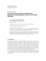
Figure 1: The block diagram of the downmixing with weighting
and delay (DWD) method.
a 9-band equalizer [15]. Rarely has been seen a theoretical

treatment with rigorous evaluation on the approaches that
have been developed for this difficult problem.
If binaural audio and the WFS are regarded as two
extremes in terms of loudspeaker channels, this paper is
focused on pragmatic and compromising approaches of
automotive audio spatializers targeted at economical cars
with four available loudspeakers for 5.1-channel input
contents. In these approaches, it is necessary to downmix
the audio signals to decrease the number of audio channels
between the inputs and the outputs [16]. By combining
various inverse filtering and the downmixing techniques, six
rendering strategies are proposed for various passengers’ sit-
ting modes. One of the six methods is based on downmixing
approaches, whereas the remaining five methods are based
on inverse filtering.
The proposed approaches have been implemented on
a real car by using a fixed-point digital signal processor
(DSP). Extensive objective and subjective experiments were
conducted to compare the presented rendering strategies for
various listening scenarios. In order to justify the statistical
significance of the results, the data of subjective listening
tests are processed by the multivariate analysis of variance
(MANOVA) [17] method, followed by the least significant
difference method (Fisher’s LSD) as a post hoc test. In light of
these tests, it is hoped that viable rendering strategies capable
of delivering compelling and immersive listening experience
in automotive environments can be found.
2. Downmixing-Based Strategy
In this section, rendering strategy based on downmixing is
presented. Given 5.1-channel input contents, a straightfor-

ward approach is to feed the input signals to the respective
loudspeakers. However, this approach often cannot deliver
satisfactory sound image duo to the asymmetric arrange-
ment of the loudspeakers/passengers in the car environment.
To balance the front and back, the downmixing with weight-
ing and delay (DWD) method is developed, as depicted in
the block diagram of Figure 1. According to the standard
downmixing algorithm stated in ITU-R BS.775-1 [18], the
center channel is weighted by 0.71 (or
−3 dB) and mixed
into the frontal channels. Similarly, the back left and the back
right surround channels are weighted by 0.71 and mixed into
the front left and the front right channels, respectively. That
is,
L
= FL + 0.71 ×C+0.71 × BL
R
= FR + 0.71 ×C+0.71 × BR.
(1)
Next, the frontal channels are weighted (0.65) and
delayed (20 millisecond) to produce the back channels.
3. Inverse Filtering-Based Approaches
Beside the aforementioned downmixing-based strategy, five
other strategies are based on inverse filtering. These design
strategies are further divided into two categories. The first
category is based on the Head-Related Transfer Functions
(HRTFs) that account for the diffraction and shadowing
effects due to the head, ears, and torso. Three rendering
strategies are developed to reproduce four virtual images
located at

±30
◦
and ±110
◦
in accordance with the 5.1
deployment stated in ITU-R Rec. BS.775-1 [18]. For the 5.1-
channel inputs and four loudspeakers, the center channel
has to be attenuated by
−3 dB and mixing into the front-left
and the front-right channels. The HRTF database measured
by the MIT Media Laboratory [19, 20] is employed as the
matching model, whereas the HRTFs measured in the car
are used as the acoustical plant. The second category named
“the point-receiver model” regards the passenger’s head as a
simple point-receiver at the center.
3.1. Multichannel Inverse Filtering. The inverse filtering
problem can be viewed from a model-matching perspective,
as shown in Figure 2. In the block diagram, x(z) is a vector of
N program inputs, v(z) is a vector of M loudspeaker inputs,
and e(z) is a vector of L error signals or control points. Also,
M(z)isanL
× N matrix of the matching model, H(z)isan
L
×M plant transfer matrix, and C(z)isanM ×N matrix of
the inverse filters. The z
−m
term accounts for the modeling
delay to ensure causality of the inverse filters. For arbitrary
inputs, minimization of the error output is tantamount to
the following optimization problem:

min
C
M −HC
2
F
,(2)
where F symbolizes the Frobenius norm [21]. Using Tikhnov
regularization, the inverse filter matrix can be shown to be
[7].
C
=

H
H
H + βI

−1
H
H
M,(3)
The regularization parameter β that weights the input
power against the performance error can be used to prevent
the singularity of H
H
H from saturating the filters. If β is too
small, there will be sharp peaks in the frequency responses
of the CCS filters, whereas if β is too large, the cancellation
performance will be rather poor. The criterion for choosing
the regularization parameter β is dependent on a preset gain
threshold [7]. Inverse Fast Fourier transforms (FFT) along

with circular shifts (hence the modeling delay) are needed to
obtain causal FIR filters.
EURASIP Journal on Audio, Speech, and Music Processing 3
z
−m
Acoustical
plant
Inverse
filters
Matching
model
Modeling
delay
+
−
M(z)
H(z)C(z)
Error
e(z)
Desired signals
d(z)
Reproduced signals
w(z)
Input signals
x(z)
Speaker
input signals
v(z)
L × N
M × NL × M

Figure 2: The block diagram of the multichannel model matching problem. L: number of control points, M: number of loudspeakers, N:
number of program inputs.
In general, it is not robust to implement the inverse
filters based on the measured room responses that usually
have many noninvertible zeros (deep troughs) [22]. In this
paper, a generalized complex smoothing technique suggested
by Hatziantoniou and Mourjopoulos [23] is employed to
smooth out the peaks and dips of the acoustical frequency
responses before the design of inverse filters.
3.2. Inverse Filtering-Based Approaches and Formulation
3.2.1. HRTF Model. The experimental arrangement for a
single passenger sitting on an arbitrary seat, for example,
the front left seat, in the car is illustrated as Figure 3. This
arrangement involves two control points at the passenger’s
ears, four loudspeakers, and four input channels. Thus, the
2
×4 acoustical plant matrix H(z) and the 2×4 matching
model matrix M(z)canbewrittenas
H
(
z
)
=
⎡
⎣
H
11
(
z
)

H
12
(
z
)
H
13
(
z
)
H
14
(
z
)
H
21
(
z
)
H
22
(
z
)
H
23
(
z
)

H
24
(
z
)
⎤
⎦
,(4)
M
(
z
)
=
⎡
⎣
HRTF
i
30
HRTF
c
30
HRTF
i
110
HRTF
c
110
HRTF
c
30

HRTF
i
30
HRTF
c
110
HRTF
i
110
⎤
⎦
,(5)
where the superscripts i and c refer to the ipsilateral and the
contralateral paths, respectively. The subscripts 30 and 110 in
the matching model matrix M(z) signify the azimuth angles
of the HRTF. The HRTFs are assumed to use symmetry, the
−HRTF
30
and −HRTF
110
are generated by swapping the ipsi-
lateral and contralateral sides of +HRTF
30
and +HRTF
110
.
The acoustical plants H(z) are the frequency response
functions between the inputs to the loudspeakers and the
outputs from the microphones mounted in the (Knowles
Electronics Manikin for Acoustic Research KEMAR’s) [19,

20] ears. This leads to a 4
×4 matrix inversion problem, which
is computationally demanding to solve. In order to yield a
more tractable solution, the current research has separated
this problem into two parts: the front side and the back
side. Specifically, the frontal loudspeakers are responsible
for generating the sound images at
±30
◦
, while the back
loudspeakers are responsible for generating the sound images
at
±110
◦
. In this approach, the plant, the matching model,
and the inverse filter matrices are given by
H
F
(
z
)
=
⎡
⎣
H
11
(
z
)
H

12
(
z
)
H
21
(
z
)
H
22
(
z
)
⎤
⎦
,
H
B
(
z
)
=
⎡
⎣
H
13
(
z
)

H
14
(
z
)
H
23
(
z
)
H
24
(
z
)
⎤
⎦
,
(6)
M
F
(
z
)
=
⎡
⎣
HRTF
i
30

HRTF
c
30
HRTF
c
30
HRTF
i
30
⎤
⎦
,
M
B
(
z
)
=
⎡
⎣
HRTF
i
110
HRTF
c
110
HRTF
c
110
HRTF

i
110
⎤
⎦
,
(7)
C
F
(
z
)
=
⎡
⎣
C
F
11
(
z
)
C
F
12
(
z
)
C
F
21
(

z
)
C
F
22
(
z
)
⎤
⎦
,
C
B
(
z
)
=
⎡
⎣
C
R
11
(
z
)
C
R
12
(
z

)
C
R
21
(
z
)
C
R
22
(
z
)
⎤
⎦
,
(8)
where superscripts F and B denote the front-side and the
back-side, respectively. The inverse matrices are calculated
using (3). In comparison with the formulation in (4)and(5),
a great saving of computation can be attained by applying
this approach. The number of the inverse filters reduces from
sixteen (one 4
×4matrix)toeight(two2×2 matrices).
To be specific, there are two +HRTF
30
–one for the
ipsilateral side (HRTF
i
30

) and another for contralateral side
(HRTF
c
30
). Both HRTFs refer to the transfer functions
between a source positioned at +30
◦
with respect to the head
center and two ears. Although the loudspeakers in the car are
not symmetrically deployed, the matching model (consisting
of
±HRTF
30
and ±HRTF
110
) of the inverse filter design in
the present study is chosen tom be symmetrical. For the
asymmetrical acoustical plants, we can calculate the inverse
4 EURASIP Journal on Audio, Speech, and Music Processing
filters using (3). The loudspeaker setups are not symmetrical
for the front left virtual sound and the front right virtual
sound and hence the acoustical plants are not symmetrical.
This results in different solutions for the inverse filters.
Next, the situation with two passengers sitting on
different seats, for example, the front left and the back right
seats, is examined. This problem involves four control points
for two passengers’ ears, four loudspeakers, and four input
channels. Following the steps from the single passenger case,
the design of the inverse filter can be divided into two parts.
Accordingly, two 4

×2 matrices of the acoustical plants, two
4
×2 matrices of the matching models, and two 2×2matrices
of the inverse filters are expressed as follows:
H
F
(
z
)
=
⎡
⎢
⎢
⎢
⎢
⎢
⎢
⎣
H
11
(
z
)
H
12
(
z
)
H
21

(
z
)
H
22
(
z
)
H
31
(
z
)
H
32
(
z
)
H
41
(
z
)
H
42
(
z
)
⎤
⎥

⎥
⎥
⎥
⎥
⎥
⎦
,
H
B
(
z
)
=
⎡
⎢
⎢
⎢
⎢
⎢
⎢
⎣
H
11
(
z
)
H
12
(
z

)
H
21
(
z
)
H
22
(
z
)
H
31
(
z
)
H
32
(
z
)
H
41
(
z
)
H
42
(
z

)
⎤
⎥
⎥
⎥
⎥
⎥
⎥
⎦
,
(9)
M
F
(
z
)
=
⎡
⎢
⎢
⎢
⎢
⎢
⎢
⎣
HRTF
i
30
HRTF
c

30
HRTF
c
30
HRTF
i
30
HRTF
i
30
HRTF
c
30
HRTF
c
30
HRTF
i
30
⎤
⎥
⎥
⎥
⎥
⎥
⎥
⎦
,
M
B

(
z
)
=
⎡
⎢
⎢
⎢
⎢
⎢
⎢
⎣
HRTF
i
110
HRTF
c
110
HRTF
c
110
HRTF
i
110
HRTF
i
110
HRTF
c
110

HRTF
c
110
HRTF
i
110
⎤
⎥
⎥
⎥
⎥
⎥
⎥
⎦
,
(10)
C
F
(
z
)
=
⎡
⎣
C
F
11
(
z
)

C
F
12
(
z
)
C
F
21
(
z
)
C
F
22
(
z
)
⎤
⎦
,
C
B
(
z
)
=
⎡
⎣
C

R
11
(
z
)
C
R
12
(
z
)
C
R
21
(
z
)
C
R
22
(
z
)
⎤
⎦
.
(11)
The subscripts of H
ij
(z ), are as follows i = 1,2referstothe

left and right ears of the passenger 1, i
= 3,4 refers to the
left and the right ears of the passenger 2, and j
= 1,2,3,4
refers to the four loudspeakers. In the 4
×2matricesM
F
(z )
and M
B
(z ), the first and second rows are identical to the
third and fourth rows. Specifically, the rows 1 and 2 are for
passenger 1 while the rows 3 and 4 are for passenger 2. The
two HRTF inversion methods outlined in (6)–(8)and(9)–
(11) were used to generate the following test.
HRTF-Based Inverse Filtering for Single Passenger. For the
rendering mode with a single passenger and 5.1-channel
input, the HRTF-based inverse-filtering (HIF1) method is
H
12
H
13
H
22
H
23
H
14
H
24

H
11
H
21
Figure 3: The geometrical arrangement for the HRTF-based
rendering approaches.
FL
FL
FR
RR
FR
C
RL
RR
RL
z
−D
w
2
w
1
z
−D
z
−D
z
−D
w
2
w

3
w
3
C
F
11
C
F
21
C
F
12
C
F
22
C
R
11
C
R
21
C
R
22
C
R
12
Figure 4: The block diagrams of the HRTF-based inverse filtering
for single passenger (HIF1) method, the HRTF-based inverse
filtering for two passengers (HIF2) method, and the HRTF-based

inverse filtering for two passengers by filter superposition (HIF2-S)
method.
developed. The block diagram is shown in Figure 4. For the
5.1-channel inputs and four loudspeakers, the center channel
has to be attenuated by
−3 db before mixing into the front-
left and the front-right channels. Next, two frontal channels
and two back channels are fed to the respective inverse filters.
Prior to designing the inverse filters, the acoustical plants
EURASIP Journal on Audio, Speech, and Music Processing 5
Loudspeaker 2
Loudspeaker 3 Loudspeaker 4
Loudspeaker 1
H
3
H
4
H
1
H
2
Figure 5: The geometrical arrangement for the point receiver-based
rendering approaches.
H(z )in(6) are measured. The matching model matrices and
the inverse filters are given in (7)and(8). The weight
= 0.45
and delay
= 4 ms are used in mixing the four-channel inputs
into the respective channels. It is noted that this procedure
will also be applied to the following inverse-filtering-based

methods.
HRTF-Based Inverse Filtering (HIF2) for Two Passengers.
In this section, two HRTF-based inverse filtering strategies
designed for two passengers and 5.1-channel input are pre-
sented. The first approach named the HIF2 method considers
four control points for two passengers. The associated system
matrices take the form formulated in (9)to(11). The two
2
×2 inverse filter matrices are calculated as previously. The
block diagram of the HIF2 method follows that of the HIF1
method.
HRTF-Based Inverse Filtering (HIF2-S) for Two Passengers. In
this approach, the inverse filters are constructed by superim-
posing the filters used in the single-passenger approach. That
is
C
F
position 1&2
(
z
)
= C
F
position 1
(
z
)
+ C
F
position 2

(
z
)
C
B
position 1&2
(
z
)
= C
B
position 1
(
z
)
+C
B
position 2
(
z
)
.
(12)
This approach is named the HIF2-S method. In (12), the
design procedures of the HIF2-S method are divided into two
steps. First, the inverse filters for a single passenger sitting
on respective positions are designed. Next, by adding the
filter coefficients obtained in the first step, two 2
×2inverse
filter matrices are obtained. The block diagram of the HIF2-

S method follows that of the HIF1 method.
3.2.2. Point-Receiver Model. In this section, a scenario is
considered. It is when a single passenger sits on an arbitrary
seat in the car, for example, the front left seat, as shown
z
−D
w
2
w
1
z
−D
z
−D
z
−D
w
2
w
3
w
3
C
1
C
2
C
3
C
4

FL
FR
RL
RR
FL
FR
C
RL
RR
Figure 6: The block diagrams of the point-receiver-based inverse
filtering for single passenger (PIF1) method and the point-receiver-
based inverse filtering for two passengers by filter superposition
(PIF2-S) method.
in Figure 5. In this setting, rendering is aimed at what we
called the “control point” at the passenger’s head center
position. A monitoring microphone instead of the KEMAR
is required in measuring the acoustical plants and the
matching model responses between the input signals and the
control points. Hence, the acoustical plant is treated in this
approach as four independent (single-input-single-output
SISO) systems. These SISO inverse filters can be calculated
by
C
m
(
z
)
=
H
∗

m
(
z
)
M
(
z
)
H
∗
m
(
z
)
H
m
(
z
)
+ β
, (13)
where H
m
(z), m = 1 ∼ 4 denotes the transfer function from
the mth loudspeaker to the control point. The frequency
response function measured using the same type of loud-
speakers in the car in an anechoic chamber is designated
as the matching model M(z). The point-receiver model was
used to generate the following test system.
Point-Receiver-Based Inverse Filtering for Single Passenger.

For the 5.1-channel input, the point-receiver-based inverse
filtering for single passenger (PIF1) method is developed.
This method mimics the concepts of the Pioneer’s MCACC
[15], but is more accurate in that an inverse filter instead
of a simple equalizer is used. The acoustical path from each
loudspeaker to the control point is modeled as a SISO system
in Figure 5. Four SISO inverse filters are calculated using
(13), with identical modeling delay. In Figure 6, the center
channel has to be attenuated before mixing into the front-
left and front-right channels. The two frontal channels and
two back channels are fed to the respective inverse filters.
6 EURASIP Journal on Audio, Speech, and Music Processing
(a) The 2-liter and 4-door sedan.
LCD
DVD player
Front-right
loudspeaker
Rear-right
loudspeaker
(b) The experimental arrangement inside the car equipped
with four loudspeakers.
Figure 7: The car used in the objective and subjective experiments.
Table 1: The descriptions of ten automotive audio rendering approaches.
Method No. input channel No. passenger Design strategy
DWD 5.1 1 or more Downmixing + weighting & delay
HIF1 5.1 1 HRTF-based inverse filtering
HIF2 5.1 2 HRTF-based inverse filtering
HIF2-S 5.1 2 HRTF-based inverse filtering
PIF1 5.1 1 Point-receiver-based inverse filtering
PIF2-S 5.1 2 Point-receiver-based inverse filtering

Point-Receiver-Based Inverse Filtering for Two Passengers.
For the rendering scenario with two passengers and 5.1-
channel input, the aforementioned filter superposition idea
is employed in the point-receiver-based inverse filtering
approach (PIF2-S). The structure of this rendering approach
is similar to those of the PIF1 approach, as shown in
Figure 6. A PIF2 system analogous to the HIF2 system
was considered in initial tests, but was eliminated from
final testing because the PIF2 approach performed badly
in an informal experiment, as compared with the other
approaches.
4. Objective and Subjective Evaluations
Objective and subjective experiments were undertaken to
evaluate the presented methods, as summarized in Table 1.
In the objective experiments, we consider only inverse-
filtering based approaches and not downmixing, and we
compared the measured inverse-filtering system transfer
function with the desired plant transfer function. Through
these experiments, it is hoped that the best strategy for
each rendering scenario can be found. For the objective
experiments, the measurements are only made as HIF1 for
the LF listener, HIF2 for the LF and BR listener, and PIF1
for the FL listener, in other words, not all configurations
listed in Ta ble 1 were tested objectively. These experiments
were conducted in an Opel Vectra 2-liter sedan (Figure 7(a))
equipped with a DVD player, a 7-inch LCD display, a
multichannel audio decoder, and four loudspeakers (two
mounted in the lower panel of the front door and two behind
the back seat). The experimental arrangement inside the
car is shown in Figure 7(b). The rendering algorithms were

implemented on a fixed-point digital signal processor (DSP),
Blackfin-533, of Analog Device semi-conductor. The GRAS
40AC microphone with the GRAS 26AC preamplifier was
used for measuring the acoustical plants.
4.1. Objective Experiments
4.1.1. The HRTF-Based Model. In this section, strategies
based on the HRTF model are examined. First, for the
scenario with a single passenger sitting in the FL seat, the
rendering approach of the HIF1 method is examined. Figures
8(a) and 8(b) show the frequency responses of the respective
frontal and back plants in the matrix form. The ijth (i
=
1,2, and j = 1,2) entry of the matrix figures represents the
respective acoustical path in (6). That is, the upper and
lower rows of the figures are measured at the left and right
ears, respectively. The left and right columns of the figures
are measured when the left-side and right-side loudspeakers
are enabled, respectively. The measured responses have been
effectively smoothed out using the technique developed
by Hatziantoniou and Mourjopoulos [23]. Comparison of
the left and the right columns of Figures 8(a) and 8(b)
reveals that head shadowing is not significant because of the
strong reflections from the boundary of the car cabin. The
frequency response of the inverse filters show that the filter
frequency responses above 6 kHz exhibit high gain because of
EURASIP Journal on Audio, Speech, and Music Processing 7
×10
4
21.510.50
FL loudspeaker to L ear

−60
−40
−20
0
20
40
Magnitude (dB)
×10
4
21.510.50
FL loudspeaker to R ear
−60
−40
−20
0
20
40
Magnitude (dB)
×10
4
21.510.50
FR loudspeaker to L ear
−60
−40
−20
0
20
40
Magnitude (dB)
×10

4
21.510.50
FR loudspeaker to R ear
−60
−40
−20
0
20
40
Magnitude (dB)
Frequency (Hz)
(a) From the frontal loudspeakers.
×10
4
21.510.50
BL loudspeaker to L ear
−60
−40
−20
0
20
40
Magnitude (dB)
×10
4
21.510.50
BL loudspeaker to R ear
−60
−40
−20

0
20
40
Magnitude (dB)
×10
4
21.510.50
BR loudspeaker to L ear
−60
−40
−20
0
20
40
Magnitude (dB)
×10
4
21.510.50
BR loudspeaker to R ear
−60
−40
−20
0
20
40
Magnitude (dB)
Frequency (Hz)
(b) From the back loudspeakers. The dotted lines and the solid lines represent the measured and the
smoothed responses.
Figure 8: The frequency responses of the HRTF-based acoustical plant at the FL seat.

8 EURASIP Journal on Audio, Speech, and Music Processing
×10
4
21.510.50
HC for HRTF
−30
◦
(L ear)
−60
−40
−20
0
20
40
Magnitude (dB)
×10
4
21.510.50
HC for HRTF
−30
◦
(R ear)
−60
−40
−20
0
20
40
Magnitude (dB)
×10

4
21.510.50
HC for HRTF +30
◦
(L ear)
−60
−40
−20
0
20
40
Magnitude (dB)
×10
4
21.510.50
HC for HRTF +30
◦
(R ear)
−60
−40
−20
0
20
40
Magnitude (dB)
Frequency (Hz)
(a) For the frontal image.
×10
4
21.510.50

HC for HRTF
−110
◦
(L ear)
−60
−40
−20
0
20
40
Magnitude (dB)
×10
4
21.510.50
HC for HRTF
−110
◦
(R ear)
−60
−40
−20
0
20
40
Magnitude (dB)
×10
4
21.510.50
HC for HRTF +110
◦

(L ear)
−60
−40
−20
0
20
40
Magnitude (dB)
×10
4
21.510.50
HC for HRTF +110
◦
(R ear)
−60
−40
−20
0
20
40
Magnitude (dB)
Frequency (Hz)
(b) For the back image.
Figure 9: The comparison of frequency response magnitudes of the HRTF-based plant-filter product and the matching model for single
passenger sitting in the FL seat. The solid lines and the dotted lines represent the matching model responses M and the plant-filter product
HC,respectively.
EURASIP Journal on Audio, Speech, and Music Processing 9
×10
4
21.510.50

HC for FL loudspeaker to FL seat (L ear)
−40
−20
0
20
40
Magnitude (dB)
×10
4
21.510.50
HC for FR loudspeaker to FL seat (L ear)
−40
−20
0
20
40
Magnitude (dB)
×10
4
21.510.50
HC for FL loudspeaker to FL seat (R ear)
−40
−20
0
20
40
Magnitude (dB)
×10
4
21.510.50

HC for FR loudspeaker to FL seat (R ear)
−40
−20
0
20
40
Magnitude (dB)
×10
4
21.510.50
HC for FL loudspeaker to BR seat (L ear)
−40
−20
0
20
40
Magnitude (dB)
×10
4
21.510.50
HC for FL loudspeaker to BR seat (R ear)
−40
−20
0
20
40
Magnitude (dB)
×10
4
21.510.50

HC for FR loudspeaker to BR seat (L ear)
−40
−20
0
20
40
Magnitude (dB)
×10
4
21.510.50
HC for FR loudspeaker to BR seat (R ear)
−40
−20
0
20
40
Magnitude (dB)
Frequency (Hz)
(a) For the frontal image.
Figure 10: Continued.
10 EURASIP Journal on Audio, Speech, and Music Processing
×10
4
21.510.50
HC for BL loudspeaker to FL seat (L ear)
−40
−20
0
20
40

Magnitude (dB)
×10
4
21.510.50
HC for BR loudspeaker to FL seat (L ear)
−40
−20
0
20
40
Magnitude (dB)
×10
4
21.510.50
HC for BL loudspeaker to FL seat (R ear)
−40
−20
0
20
40
Magnitude (dB)
×10
4
21.510.50
HC for BR loudspeaker to FL seat (R ear)
−40
−20
0
20
40

Magnitude (dB)
×10
4
21.510.50
HC for BL loudspeaker to BR seat (L ear)
−40
−20
0
20
40
Magnitude (dB)
×10
4
21.510.50
HC for BL loudspeaker to BR seat (R ear)
−40
−20
0
20
40
Magnitude (dB)
×10
4
21.510.50
HC for BR loudspeaker to BR seat (L ear)
−40
−20
0
20
40

Magnitude (dB)
×10
4
21.510.50
HC for BR loudspeaker to BR seat (R ear)
−40
−20
0
20
40
Magnitude (dB)
Frequency (Hz)
(b) For the back image.
Figure 10: The comparison of frequency response magnitudes of the HRTF-based plant-filter product and the matching model for two
passengers sitting in the FL and RR seats. The solid lines and the dotted lines represent the matching model responses M and the plant-filter
product HC,respectively.
EURASIP Journal on Audio, Speech, and Music Processing 11
×10
4
21.510.50
FL loudspeaker to control point
−40
−20
0
20
Magnitude (dB)
×10
4
21.510.50
BL loudspeaker to control point

−40
−20
0
20
Magnitude (dB)
×10
4
21.510.50
FR loudspeaker to control point
−40
−20
0
20
Magnitude (dB)
×10
4
21.510.50
BR loudspeaker to control point
−40
−20
0
20
Magnitude (dB)
Frequency (Hz)
Figure 11: The frequency responses of the point-receiver-based acoustical plants for single passenger sitting in the FL seat. The dotted lines
and the solid lines represent the measured and the smoothed responses, respectively.
the poor high-frequency response of the back loudspeakers.
To regularize the inverse filters, the gain is always kept below
6 dB to prevent from overloading the loudspeakers. The solid
lines in Figures 9(a) and 9(b) represent the HRTF pair at 30

◦
and 110
◦
, respectively, whereas the dotted lines represent the
plant-filter product, H(e
jω
)C(e
jω
). The agreement between
these two sets of responses is generally good below 6 kHz
except for the back loudspeaker. This is because the inverse
filters are gain-limited in the frequencies at which the plants
have significant roll-off.
Next, the scenario of two passengers sitting in the FL
and BR seats is examined. The preceding design procedure of
inverse filers is employed in the HIF2 method. These plots are
arranged in matrix form, where the ijth (i
= 1 ∼ 4, j = 1, 2)
entry represents the respective inverse filter in (11). Similar
to the result for a single passenger, the frequency response of
inverse filters exhibit high gain in high frequencies. Figures
10(a) and 10(b) compare the plant-filter product and the
matching model for the frontal and the back virtual images,
respectively. Both the ipsilateral and contralateral responses
of the plant-filter product did not fit the matching model
responses very well. This is due to the fact that it is difficult
to invert the nonsquare 4
×2 acoustical plant matrix H.A
further comparison of the HIF2 and HIF2-S methods will be
presented in the following subjective tests.

4.1.2. The Point-Receiver-Based Model. First, the scenario of
a single passenger sitting in the FL seat is examined. Figure 11
shows the frequency responses between the four loudspeak-
ers and the microphone placed at the center position of
passenger’s head (the control point). Figures 11(a) and 11(b)
show the measured and the smoothed frequency responses
of the acoustical plants when the FL and the FR loudspeakers
are enabled. Figures 11(c) and 11(d) show the measured and
the smoothed frequency responses of the acoustical plants
when the BL and BR loudspeakers are enabled, respectively.
Both the measured frequency responses were smoothed out
by using the technique developed by Hatziantoniou and
Mourjopoulos [23]. Similar to the results of the preceding
HRTF-based approach, the frequency response of the filters
12 EURASIP Journal on Audio, Speech, and Music Processing
Table 2: The descriptions of four subjective listening experiments.
Experiment I II
Input content 5.1-channel 5.1-channel
No. passenger 1 2
Processing method
DWD DWD
HIF1 HIF2
PIF1 HIF2-S
PIF2-S
Reference
FL
in
+0.7 × C
in
→ FL

out
FR
in
+0.7 × C
in
→ FR
out
BL
in
→ BL
out
BR
in
→ BR
out
Anchor Summation of all lowpass filtered inputs → All outputs
Table 3: The definitions of the subjective attributes.
Attribute Description
Preference Overall preference in considering timbral and spatial attributes
Fullness Dominance of low-frequency sound
Brightness Dominance of high-frequency sound
Artifacts Any extraneous disturbances to the signal
Localization Determination by a subject of the apparent source direction
Frontal The clarity of the frontal image or the phantom center
Proximity The sound is dominated by the loudspeaker closest to the subject
Envelopment Perceived quality of listening within a reverberant environment
Table 4: The summary of the rendering strategies recommended
for various listening scenarios.
Passenger Number input channel Strategy
1FL 4 HIF1

1BR 4 PIF1
24DWD
shows high gain above 10 kHz due to the high-frequency
roll-off of the back loudspeakers. Figure 12 shows the
inverse plant-filter product, H(e
jω
)C(e
jω
). The responses are
generally in good agreement below 10 kHz except for the
back loudspeakers.
4.2. Subjective Experiments. Subjective listening experiments
were conducted to investigate the six audio rendering meth-
ods presented in Sections 2 and 3, according to a modified
double-blind Multi-Stimulus test with Hidden Reference and
a hidden Anchor (MUSHRA) [24]. The case designs of
experiments are described in Table 2. In these experiments,
four 5.1-channel music videos and a movie in Dolby Digital
format were used. In the (“Dragon heart”) movie, a scene
with the dragon flying in a circle as a moving sound source
is selected to be the stimulus for evaluating the attribute
localization.
Eight subjective attributes employed in the tests, includ-
ing preference, the timbral attributes (fullness, brightness,
artifact) and the spatial attributes (localization, frontal image,
proximity, envelopment) are summarized in Ta b le 3.Forty
subjects participating in the listening tests were instructed
with definitions of the subjective attributes and the proce-
dures before the tests. The subjects were asked to respond
in a questionnaire after listening, with the aid of a set of

subjective attributes measured on an integer scale from
−3
to 3. Positive, zero, and negative scores indicate perceptually
improvement, no difference, and degradation, respectively,
of the signals processed by the rendering algorithm under
test. The order to grade the attributes is randomized except
that the attribute preference is always graded last. In order
to access statistical significance of the test results, the scores
were further processed by using the MANOVA. If the
significance level is below 0.05, the difference among all
methods is considered statistically significant and will be
processed further by the Fisher’s LSD post hoc test to perform
multiple paired comparisons.
4.2.1. Experiment I
Methods. Experiment I is intended for evaluating the render-
ing algorithms designed for one passenger in the FL seat or
BR seat. The DWD, HIF1, and PIF1 methods are compared in
this experiment. Because only four loudspeakers are available
in this car, the center channel of the 5.1-channel input is
attenuated by
−3 dB and mixed into the frontal channels to
serve as the hidden reference. In addition, the four channels
of input signals are summed and lowpass filtered (with 4 kHz
cutoff frequency) to serve as the anchor.
EURASIP Journal on Audio, Speech, and Music Processing 13
×10
4
21.510.50
HC for FL loudspeaker to control point
−40

−20
0
20
Magnitude (dB)
×10
4
21.510.50
HC for BL loudspeaker to control point
−40
−20
0
20
Magnitude (dB)
×10
4
21.510.50
HC for FR loudspeaker to control point
−40
−20
0
20
Magnitude (dB)
×10
4
21.510.50
HC for BR loudspeaker to control point
−40
−20
0
20

Magnitude (dB)
Frequency (Hz)
Figure 12: The comparison of frequency response magnitudes of the point-receiver-based plant-filter product and the matching model for
single passenger sitting in the FL seat. The solid lines and the dotted lines represent the matching model responses M and the plant-filter
product HC,respectively.
Results. Figures 13(a) and 13(b) show the means and spreads
of the grades on the subjective attributes for the FL position,
while Figures 13(c) and 13(d) show the results for the
BR position. For the FL position, the results of the post
hoc test indicate that the grades of the HIF1 method in
preference and fullness are significantly higher than those of
the DWD and the PIF1 methods. In brightness, only the
grade of PIF1 methods is significantly higher than the hidden
reference, while no significant difference between the DWD
method and the HIF1 method is found. In addition, there
is no significant difference among methods in the attributes
artifact, localization, proximity and envelopment. In the
attribute frontal, however, the inverse filter-based methods
received significantly higher grades than the hidden reference
and the DWD method.
In the BR position, there is no significant difference
among all the methods in fullness, artifact, and localization.
However, the grades received in preference and brightness
using the inverse filtering-based method is significantly
higher than the grades obtained using the other methods. In
addition, all rendering methods received significantly higher
grades in proximity than the hidden reference. Finally, only
the HIF1 method significantly outperformed the hidden
reference in envelopment. In general, all grades received are
higher for the back seat than for the front seat. The HIF1

method received the highest grades in most attributes, espe-
cially in the spatial attributes. Considering the computation
complexity, the PIF1 method is also a viable approach second
to the HIF1 method because it received high grades in many
attributes as well.
4.2.2. Experiment II
Methods. Experiment II is intended for evaluating the
rendering algorithms designed for two passengers in the
FL seat and BR seat and the 5.1-channel input. Four
methods including the DWD method, the HIF2 method, the
HIF2-S method, and the PIF2-S method are compared in
14 EURASIP Journal on Audio, Speech, and Music Processing
H.R.An.PIF1HIF1DWD
Position: FL
1 passenger, 5.1-ch input
−4
−3
−2
−1
0
1
2
3
Grade
(a) )The first four attributes for the FL seat.
H.R.An.PIF1HIF1DWD
Position: FL
1 passenger, 5.1-ch input
−3.5
−3

−2.5
−2
−1.5
−1
−0.5
0
0.5
1
1.5
2
2.5
3
Grade
(b) The last four attributes for the FL seat.
H.R.An.PIF1HIF1DWD
Position: RR
1 passenger, 5.1-ch input
−4
−3
−2
−1
0
1
2
3
Grade
Preference
Fullness
Brightness
Artifact

(c) The first four attributes for the RR seat.
H.R.An.PIF1HIF1DWD
Position: RR
1 passenger, 5.1-ch input
−4
−3
−2
−1
0
1
2
3
4
Grade
Localization
Frontal
Proximity
Envelopment
(d) The last four attributes for the RR seat.
Figure 13: The means and spreads (with 95% confidence intervals) of the grades on the subjective attributes for Experiment I.
H.R.An.PIF2-SHIF2-SHIF2DWD
Position: FL and RR
2 passenger, 5.1-ch input
−4
−3
−2
−1
0
1
2

3
4
Grade
Preference
Fullness
Brightness
Artifact
(a) The first four attributes.
H.R.An.PIF2-SHIF2-SHIF2DWD
Position: FL and RR
2 passenger, 5.1-ch input
−4
−3
−2
−1
0
1
2
3
4
Grade
Localization
Frontal
Proximity
Envelopment
(b) The last four attributes.
Figure 14: The means and spreads (with 95% confidence intervals) of the grades on the subjective attributes for Experiment II.
EURASIP Journal on Audio, Speech, and Music Processing 15
this experiment. The hidden reference and the anchor are
identical to those defined in Experiment I.

Results. Figure 14 shows the means and spreads of the grades
of all subjective attributes. The results of the post hoc test
reveals that there is no significant difference between the
DWD method and HIF2-S method, while both grades in
preference are significantly higher than the hidden reference.
In fullness and proximity, no significant difference was found
among all proposed methods. In brightness, results similar
to Experiment I are obtained. The inverse filtering-based
methods received significant higher grades than the hidden
reference, albeit there is no significant difference among the
inverse filtering-based methods methods. The HIF2 method
received very low grade in artifact, implying that artifacts
are audible. This could be due to the problem of inverse
filter design for the nonsquare acoustical system. In frontal
and localization, all methods received significantly higher
grades than the hidden reference. Finally, the HIF2-S method
has attained the best performance in envelopment among all
methods. Overall, the HIF2-S method is the preferred choice
for spatial quality, which is contrary to our expectation that
more inverse filters (HIF2) should yield better performance.
On the other hand, in terms of computation complexity and
rendering performance, the DWD method is an adequate
choice for the two-passenger scenario.
5. Conclusions
A comprehensive study has been conducted to explore
various automotive audio processing approaches. Tabl e 4
summarizes the conclusions on rendering strategies which
can be drawn from the performed listening tests according
to the number of passengers.
First, for the rendering scenario with a single passenger

and the 5.1-channel inputs, the HIF1 method is suggested
for the passenger sitting in the FL seat, whereas the PIF1
method would be the preferred choice for the passenger
sitting in the BR seat. Second, for the two-passenger
scenario, the HIF2-S method received high grade in most
subjective attributes. However, no significant difference in
the attributes preference, brightness, artifact, localization and
frontal was found between the DWD method and the HIF2-
S method. Considering the computational complexity, the
DWD method should be the most preferred choice for
the two-passenger scenario. Overall, the inverse filtering
approaches did not perform as well for the multipassenger
scenario as it did for the single passenger scenario. The
number of inverse filters increases drastically with number
of passengers, rendering approaches of this kind impractical
in automotive applications.
Acknowledgments
The work was supported by the National Science Council
in Taiwan, China, under the project no. NSC91-2212-E009-
032.
References
[1] Y. Kahana, P. A. Nelson, and S. Yoon, “Experiments on the
synthesis of virtual acoustic sources in automotive interiors,”
in Proceedings of the 16th International Conference on Spatial
Sound Reproduction and Applications of the Audio Engineer ing
Society, Paris, France, March 1999.
[2] B. Crockett, M. Smithers, and E. Benjamin, “Next generation
automotive sound research and technologies,” in Proceedings
of the 120th Convention of Audio Engineering Society, Paris,
France, 2006, paper no. 6649.

[3] M. R. Bai and C. C. Lee, “Comparative study of design
and implementation strategies of automotive virtual surround
audio systems,” to appear in Journal of the Audio Engineering
Society.
[4] P. Damaske and V. Mellert, “A procedure for generating
directionally accurate sound images in the upper-half space
using two loudspeakers,” Acoustica, vol. 22, pp. 154–162, 1969.
[5] D. R. Begault, 3-D Sound for Virtual Reality and Multimedia,
AP Professional, Cambridge, Mass, USA, 1994.
[6] W. G. Gardner, “Transaural 3D audio,” Tech. Rep. 342, MIT
Media Laboratory, 1995.
[7] M. R. Bai and C C. Lee, “Development and implementation
of cross-talk cancellation system in spatial audio reproduction
based on subband filtering,” Journal of Sound and Vibration,
vol. 290, no. 3-5, pp. 1269–1289, 2006.
[8] M. R. Bai and C C. Lee, “Objective and subjective analysis of
effects of listening angle on crosstalk cancellation in spatial
sound reproduction,” The Journal of the Acoustical Society of
America, vol. 120, no. 4, pp. 1976–1989, 2006.
[9] M. R. Bai, G Y. Shih, and C C. Lee, “Comparative study of
audio spatializers for dual-loudspeaker mobile phones,” The
Journal of the Acoustical Society of America, vol. 121, no. 1, pp.
298–309, 2007.
[10] T. Takeuchi and P. A. Nelson, “Optimal source distribution
for binaural synthesis over loudspeakers,” The Journal of the
Acoustical Society of America, vol. 112, no. 6, pp. 2786–2797,
2002.
[11] D. Menzies and M. Al-Akaidi, “Nearfield binaural synthesis
and ambisonics,” TheJournaloftheAcousticalSocietyof
America, vol. 121, no. 3, pp. 1559–1563, 2007.

[12] P A. Gauthier, A. Berry, and W. Woszczyk, “Sound-field
reproduction in-room using optimal control techniques:
simulations in the frequency domain,” The Journal of the
Acoustical Society of America, vol. 117, no. 2, pp. 662–678,
2005.
[13] T. Betlehem and T. D. Abhayapala, “Theory and design of
sound field reproduction in reverberant rooms,” The Journal
of the Acoustical Society of America, vol. 117, no. 4, pp. 2100–
2111, 2005.
[14] G. Theile and H. Wittek, “Wave field synthesis: a promising
spatial audio rendering concept,” Acoustical Science and Tech-
nology, vol. 25, no. 6, pp. 393–399, 2004.
[15] Pioneer, “MCACC Multi-Channel Acoustic Calibration,”
August 2008, />PressRoom/Press+Releases/Car+Audio+Video/Computer+
Technology+and+Car+Audio+Converge+in+Pioneer+
Single+with+Hard+Disk+Drive%2C+Memory+Stick%2C+
MP3+Playback.
[16] M. R. Bai and G Y. Shih, “Upmixing and downmixing
two-channel stereo audio for consumer electronics,” IEEE
Transactions on Consumer Electronics, vol. 53, no. 3, pp. 1011–
1019, 2007.
16 EURASIP Journal on Audio, Speech, and Music Processing
[17] S. Sharma, Applied Multivariate Techniques, John Wiley &
Sons, New York, NY, USA, 1996.
[18] ITU-R Rec. BS.775-1, “Multi-channel stereophonic sound
system with or without accompanying picture,” International
Telecommunications Union, Geneva, Switzerland, 1994.
[19] W. G. Gardner and K. D. Martin, “KEMAR HRTF
measurements,” MIT’s Media Lab, August 2008,
/>[20] W. G. Gardner and K. D. Martin, “HRTF measurements of a

KEMAR,” The Journal of the Acoustical Society of America, vol.
97, no. 6, pp. 3907–3908, 1995.
[21] B. Noble, Applied Linear Algebra, Prentice-Hall, Englewood
Cliffs, NJ, USA, 1988.
[22] P. D. Hatziantoniou and J. N. Mourjopoulos, “Errors in real-
time room acoustics dereverberation,” Journal of the Audio
Engineering Society, vol. 52, no. 9, pp. 883–899, 2004.
[23] P. D. Hatziantoniou and J. N. Mourjopoulos, “Generalized
fractional-octave smoothing of audio and acoustic responses,”
Journal of the Audio Engineering Society, vol. 48, no. 4, pp. 259–
280, 2000.
[24] ITU-R BS.1534-1, “Method for the subjective assessment
of intermediate sound quality (MUSHRA),” International
Telecommunications Union, Geneva, Switzerland, 2001.