báo cáo hóa học:" Research Article Audio Query by Example Using Similarity Measures between Probability Density Functions of Features" potx

Hindawi Publishing Corporation
EURASIP Journal on Audio, Speech, and Music Processing
Volume 2010, Article ID 179303, 12 pages
doi:10.1155/2010/179303

Research Article
Audio Query by Example Using Similarity Measures between
Probability Density Functions of Features
Marko Hel´ n and Tuomas Virtanen (EURASIP Member)
e
Department of Signal Processing, Tampere University of Technology, Korkeakoulunkatu 1, 33720 Tampere, Finland
Correspondence should be addressed to Marko Hel´ n, marko.helen@tut.fi
e
Received 22 May 2009; Revised 14 October 2009; Accepted 9 November 2009
Academic Editor: Bhiksha Raj
Copyright © 2010 M. Hel´ n and T. Virtanen. This is an open access article distributed under the Creative Commons Attribution
e
License, which permits unrestricted use, distribution, and reproduction in any medium, provided the original work is properly
cited.
This paper proposes a query by example system for generic audio. We estimate the similarity of the example signal and the
samples in the queried database by calculating the distance between the probability density functions (pdfs) of their frame-wise
acoustic features. Since the features are continuous valued, we propose to model them using Gaussian mixture models (GMMs) or
hidden Markov models (HMMs). The models parametrize each sample efficiently and retain sufficient information for similarity
measurement. To measure the distance between the models, we apply a novel Euclidean distance, approximations of KullbackLeibler divergence, and a cross-likelihood ratio test. The performance of the measures was tested in simulations where audio
samples are automatically retrieved from a general audio database, based on the estimated similarity to a user-provided example.
The simulations show that the distance between probability density functions is an accurate measure for similarity. Measures based
on GMMs or HMMs are shown to produce better results than that of the existing methods based on simpler statistics or histograms
of the features. A good performance with low computational cost is obtained with the proposed Euclidean distance.

1. Introduction
The enormous growth of personal and on-line multimedia content has created the need for tools of automatic

database management. Such management tools include,
for instance, query by humming or query by example,
multimedia classification, and speaker recognition. Query
by example is an audio retrieval task where a user provides
an example signal and the retrieval system returns similar
samples from the database. The main problem in the
query by example and the other above content management
applications is to determine the similarity between two
database items.
The fundamental problem when measuring the similarity between audio samples is the imperfect definition of
similarity. For example, a human can judge the similarity
of two speech signals by the topic of the speech, by the
speaker identity, or by any sounds on the background. There
are retrieval approaches where the imperfect definition of
similarity is circumvented differently. First, the similarity
criterion can be defined beforehand. For example, query

by humming [1, 2] retrieves pieces of music which have a
musically similar melody to an input humming. Query-bybeat-boxing [3], on the other hand, aims at retrieving music
pieces which are rhythmically similar to the example. These
retrieval methods are based on extracting features which are
tuned for the particular retrieval problem.
Second, supervised classification can be used to classify
each database signal into a predefined class, for instance,
to speech, music, and environmental sounds. Supervised
classification in general has been widely studied, and audio
classifiers typically employ neural networks [4] or hidden
Markov models (HMMs) [5] on frame-wise features. In
general audio classification, extracting features in short
(∼40 ms) frames has turned out to produce good results (see

Section 2.1 for detailed discussion).
Since the above approaches define the similarity beforehand, they limit the applicability of the method to a
certain application area or to certain classes of signals. The
generic query by example of audio does not restrict the
type of signals, but aims at finding similarity criteria which
correlates with the perceptual similarity in general [6, 7].


2
The combination of the above mentioned methods have
also been used. Kiranyaz et al. made initial segmentation and
supervised classification into four predefined classes, after
which query by example was applied to samples, which were
classified into the same class [8]. For image databases, also
using multiple examples [9] and user feedback [10] have
been suggested.
This paper proposes a query by example system for
generic audio. Section 2 gives an overview of the system and
previous similarity measures. We observe that the similarity
of audio signals can be measured by the difference between
the probability density functions (pdfs) of their frame-wise
features. The empirical pdfs of continuous-valued features
cannot be estimated directly, but they are modeled using
Gaussian mixture models (GMMs). A GMM parametrizes
each sample efficiently with small number of parameters,
retaining the necessary information for similarity measurement. An overview of other applications utilizing GMMs in
the music information retrieval can be found in [11].
In Section 3 we present similarity measures between pdfs
parametrized by GMMs. We propose a novel method for
calculating the Euclidean distance between GMMs with full

covariance matrices. We also present approximations for the
Kullback-Leibler divergence between GMMs, which have not
been previously used in audio similarity measurement. A
cross-likelihood test is presented and extended to hidden
Markov models, which allow modeling temporal characteristics of the signals. Simulation experiments on a database
consisting of wide range of sounds were conducted, and the
distance measures between pdfs are shown to outperform the
existing methods in audio retrieval task in Section 4.

2. Query by Example
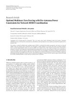
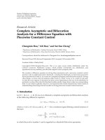
Figure 1 illustrates the block diagram of the query by
example system. An example signal is given by a user. A set
of features is extracted, and GMM or HMM is trained for the
example signal and for each database signal. The similarity
between the example and each database signal is estimated
by calculating a distance measure between their GMMs or
HMMs, and the signals having the smallest distance are
retrieved as similar to example signal.
2.1. Feature Extraction. Feature extraction aims at modeling
the perceptually most relevant information of a signal using
only a small number of features. In audio classification,
features are usually extracted in short (20–60 ms) frames,
and typically they parametrize the spectrum of the sound.
In comparison to the time-domain signal, the spectrum
correlates better with the human sound perception, and
the human auditory system has been found to perform
frequency analysis [12, pages 20–53]. The most commonly
used features in audio classification are Mel-frequency
cepstral coefficients (MFCCs) which were used for example
by Mandel and Ellis [13].

In our earlier studies [6, 7], different feature sets
were tested in general audio retrieval, and based on the
experiments the best feature set was chosen. Features were

EURASIP Journal on Audio, Speech, and Music Processing

Example
signal

Database

Feature
extraction

Feature
extraction

Estimate
GMM/HMM

Estimate
GMMs/HMMs

Similarity
estimation

Sort by
similarity

Similar

database
samples

Figure 1: Query by example system overview.

MFCCs (the first three coefficients were found to give the best
results), spectral spread, spectral flux, harmonic ratio [14],
maximum autocorrelation lag, crest factor, noise likeness
[15], total energy, and variance of instantaneous power. Even
though the feature set was tuned for a particular data set
and similarity measures, the evaluated distance measures are
general and can be applied to any set of features. In more
specific retrieval tasks it is likely that better results will be
obtained by using feature sets tuned for the particular tasks.
2.2. Previous Similarity Measures. Previous distance measures have used some statistical measures (mean, covariance,
etc.) of the features (see Sections 2.2.1 and 2.2.2) or quantized the feature vectors and then measured the similarity by
the distance between feature histograms, as will be explained
in Section 2.2.3. Recently, specific distance measures between
the pdfs of the feature vectors has been observed to be good
similarity measures [7, 16–18]. Section 3 describes distance
measures which can be calculated between pdfs parametrized
by GMMs.
2.2.1. Mahalanobis Distance. Mahalanobis distance calculates the distance between two samples based on their mean
feature vectors µA and µB , and the covariance matrix Σ of
the features across all samples in the database. The distance
is given as
DM µA , µB = µA − µB

T

Σ−1 µA − µB .

(1)

If the distribution of feature vectors of all observations
is ellipsoidal, then the Mahalanobis distance between two
mean vectors in feature space is dependent on the distance
along each feature dimension but also on the variance of that


EURASIP Journal on Audio, Speech, and Music Processing
feature dimension. This property makes the Mahalanobis
distance independent of the scale of the features. In supervised classification of music, Mandel and Ellis [13] used
a version of Mahalanobis distance, where the mean vector
consisted of all the entries of the sample-wise mean vector
and covariance matrix.
2.2.2. Bayesian Information Criterion. The Bayesian information criterion (BIC), which is a statistical criterion for
model selection, has been used especially with speech
material to segment and cluster a database [19]. BIC has
been used to measure the changing point in audio by having
two hypotheses: the first assumes that the whole sequence is
generated by a single Gaussian model, whereas the second
assumes that two segments separated by a changing point
are generated by two different Gaussian models. The BIC
difference between the hypotheses is
ΔBIC = T log(|Σ|) − TA log(|ΣA |) − TB log(|ΣB |)
−λ

1
1

d + d(d + 1) log(T),
2
2

(2)

where T is the total number of observations, TA is the
number of observations in sequence A, and TB is the number
of observations in sequence B. Σ, ΣA , and ΣB are the
covariance matrices of all the observations, sequence A, and
sequence B, respectively. d is the number of dimensions and
λ is the penalty factor to compensate for small sample sizes.
A changing point is detected if the BIC measure is above zero
[20].
2.2.3. Histogram Method. Kashino et al. [21] proposed
quantizing the frame-wise feature vectors and estimating
the similarity of two audio samples by calculating distance
between feature histograms of the samples. The centers for
quantization levels were found using the Linde-Buzo-Gray
[22] vector quantization algorithm. The feature histogram
for each sample was generated by calculating the amount
of frame-wise feature values falling on each quantization
level. The quantization level of a sample was chosen by
measuring the Euclidean distance between feature vector and
the center of each level and choosing the level that minimizes
the distance. Finally, the similarity between samples was
estimated by calculating the chosen distance (e.g., L1 -norm
or L2 -norm) between feature histograms.
The use of histograms is very flexible and straightforward
compared to other distance measures between distributions,

because practically any distance measure can be used to
calculate the distance between histogram bins. However,
a problem of using a quantized version of probability
distribution is that even if two feature vectors are closely
spaced, it is possible that they fall in a different quantization
level. Since each histogram bin is used independently, the
resulting quantization error may have a negative effect on the
performance of the similarity measure.
2.3. Query Output. After feature extraction the chosen
distance measure between the feature vectors of the example

3
and each database sample is calculated. Samples having the
smallest distances are considered as similar and are retrieved
to the user. There are two main possibilities for this. The
first is the k-nearest neighbor (k-NN) query, which retrieves
a fixed number of samples having the shortest distance to
the example [23]. The second is the -range query, which
retrieves all the samples having a shorter distance to the
example than a predefined threshold [23].
In an optimal situation, the -range query can retrieve all
the similar samples, whereas the k-NN query always retrieves
a fixed number of samples. Furthermore, in the k-NN query
the whole database has to be browsed before any samples
can be retrieved but in the -range query the samples can be
retrieved already during the query processing. On the other
hand, finding the threshold in the -range query is a complex
task and it might require estimating all the distances between
database samples before the actual query. One possibility for
estimating the threshold was suggested by Kashino et al. [21].

They determined the threshold as t = μ + σc, where μ is the
mean, σ is the standard deviation of all distances, and c is an
empirically determined constant.

3. Distribution Based Distance Measures
The distance between the pdfs of feature vectors has
been observed to be a good similarity measure [7, 16–
18]: the smaller the distance, the more similar are the
signals. Most commonly used audio features are continuous
valued, thus distance measures for continuous probability
distributions are required. A fundamental problem when
using continuous-valued features is that the empirical pdf
cannot be represented as a histogram of samples, but it has
to be approximated by a model.
We model the pdfs using GMMs or HMMs and
then calculate the distance between samples from the
model parameters. GMM for the features is explained
in Section 3.1, and Section 3.2 proposes a method for
calculating the Euclidean distance between full-covariance
GMMs. Section 3.3 presents methods for approximating
the Kullback-Leibler divergence between GMMs. Section 3.4
presents the likelihood ratio test based similarity measure,
which is then extended for HMMs. The section also shows
the connection of the methods to likelihood-ratio test and
maximum likelihood classification.
3.1. Gaussian Mixture Model for the Features. GMMs are
commonly used to model continuous pdfs, since they can
flexibly approximate arbitrary distributions. A GMM for a
feature vector x is defined as
I

p(x) =
i=1

wi N x; µi , Σi ,

(3)

where wi is the weight of the ith Gaussian component, I is
the number of components, and
N x; µi , Σi =

1
(2π)

N/2

|Σi |

exp −

1
x − µi
2

T

Σi−1 x − µi
(4)

4

EURASIP Journal on Audio, Speech, and Music Processing

is the multivariate normal distribution with mean vector µi
and covariance matrix Σi . N is the dimensionality of the
feature vector. The weights wi are nonnegative and sum to
unity. The distribution of the ith component of GMM is
referred as p(x)i = N (x; µi , Σi ).
The similarity is measured between two signals, both
of which are divided into short (e.g., 40 ms) frames and a
feature vector is extracted in each frame. A = [a1 , . . . , aTA ]
and B = [b1 , . . . , bTB ] denote the feature sequence matrices
of two signals, where TA and TB are the number of frames in
signal A and B, respectively. Here we do not restrict ourselves
to a certain set of features. An example of a possible set of
features is given in Section 2.1.
For the two observation sequences A and B, the parameters of two GMMs are estimated using the expectation maximization (EM) algorithm [24]. Let us denote the resulting
pdf of signal A and B by pA (x) and pB (x), respectively. IA and
IB are the number of Gaussian components, and wiA and wiB
are the weights of the ith component in GMM A and GMM
B, respectively.
3.2. Euclidean Distance between GMMs. The squared
Euclidean distance e between two distributions pA (x) and
pB (x) can be calculated in closed form. In [7] we derived
the calculations for diagonal-covariance GMMs, and extend
here the method for full-covariance GMMs.
The Euclidean distance is obtained by integrating the
squared difference over the whole feature space:

∞

e=

−∞

∞

···

−∞

2

pA (x) − pB (x) dx1 · · · dxN ,

(5)

where xi denotes the ith feature. To simplify the notation, we
rewrite the above multiple integral as
∞

e=

−∞

2

pA (x) − pB (x) dx.

(6)

By writing the pdfs explicitly as weighted sums of
Gaussians, the above equals
e=

∞
−∞

⎡
⎣

IA

IB

wiA pA (x)i
i=1

−

⎤2

wB pB (x) j ⎦
j

eBB =

eAB =

∞

dx.

∞

(8)

wiA wA Qi, j,A,A ,
j
i=1 j =1
IB

IB

wiB wB Qi, j,B,B ,
j

eBB =

(10)

i=1 j =1
IA IB

wiA wB Qi, j,A,B .
j

eAB =

i=1 j =1

Finally, the squared Euclidean distance is e = eAA +eBB − 2eAB .
We observe that the Euclidean distance between two
Gaussians with means µA and µB and the same covariance
matrix Σ is equal to the Mahalanobis distance DM (1), up to
a monotonic function
⎡

⎛

e = ⎣1 − exp⎝−

DM µA , µB
4

⎞⎤
⎠⎦ ×

2
(2π)

N/2

|2Σ|

,

(11)

which preserves the order of samples when distance is used
in similarity measurement.
3.3. Kullback-Leibler Divergence. The Kullback-Leibler (KL)
divergence is an information-theoretically motivated measure between two probability distributions. The KL divergence between two distributions pA (x) and pB (x) is defined
as:
∞
−∞

pA (x) log

pA (x)
dx,
pB (x)

(12)

which can be symmetrized by adding the term
KL(pB (x)|| pA (x)).
The KL-divergence between two Gaussian distributions
[25] with means µA and µB and covariances ΣA and ΣB is
1
|Σ |
−
log B + Tr ΣB 1 ΣA
2
|ΣA |
+ µA − µB

T

−
ΣB 1 µA − µB − N .

(13)

IA IB

−∞ i=1 j =1

(9)

IA IA

eAA =

KL pA (x)|| pB (x) =

IB

−∞ i=1 j =1
∞

wiA wA pA (x)i pA (x) j dx,
j

wiB wB pB (x)i pB (x) j dx,
j

pk (x)i pm (x) j dx.

The values for the terms eAA , eBB , and eAB in (8) can now be
calculated as

IA IA

IB

−∞

(7)

j =1

−∞ i=1 j =1

∞

Qi, j,k,m =

KL pA (x)|| pB (x) =

The squared distance (5) can be written as e = eAA +eBB −
2eAB , where the three terms are defined as
eAA =

Let us denote the integral of the product of the ith
component of GMM k ∈ {A, B} and the jth component of
GMM m ∈ {A, B} by

wiA wB pA (x)i pB (x) j dx.

j

All the above terms are weighted sums of definite integrals of
the product of two normal distributions. The integrals can
be solved in closed form as shown in the appendix.

For the KL divergence between GMMs which have several Gaussian components, there is no closed-form solution. There exists some approximations, many of which
were tested by Hershey and Olsen [26]. They found that
variational approximation, Goldberger approximation, and
Monte Carlo sampling produced good results.


EURASIP Journal on Audio, Speech, and Music Processing
3.3.1. KL Variational Approximation. The variational approximation [26] of the KL divergence is given as
KLvariational pA (x)|| pB (x)
IA

wiA log

=
i=1

A commonly used modification of the above is the crosslikelihood ratio test given as
C(A, B) =

IA
A
k=1 wk exp
IB
B

j =1 w j exp

−KL pA (x)i || pA (x)k
−KL pA (x)i || pB (x) j

.
(14)

3.3.2. KL Goldberger’s Approximation. The Goldberger approximation [25] is given as
KLGoldberger pA (x)|| pB (x)
IA

wiA KL pA (x)i || pB (x)m(i) + log

=

5

i=1

wiA
,
B
wm(i)

(15)

where
m(i) = argmin KL pA (x)i || pB (x) j − log wB .
j

(16)

E(A, B) =

KLMC pA (x)|| pB (x) ≈

T
pA (xt )
1
,
log
T t=1
pB (xt )

(17)

where the random samples xt are drawn from distribution
pA (x). An accurate approximation requires a large number of
samples and is therefore computationally inefficient. In [18],
we proposed to use the samples of the observation sequence
A that were used to train the distribution pA (x). We observe
that the resulting empirical Kullback-Leibler divergence KLemp
can be written as
KLemp pA (x)|| pB (x) =

pA (A)
1
.
log

TA
pB (A)

(18)

Here pA (A) and pB (A) denote the product of frame-wise pdfs
evaluated at the points of the argument A, that is, pA (A) =
TA
TA
t =1 pA (at ) and pB (A) =
t =1 pB (at ), respectively.
3.4. Cross-Likelihood Ratio Test. Likelihood ratio test is
widely used in speech clustering and segmentation (see e.g.,
[16, 17, 27]) to measure the likelihood that two segments
are spoken by the same speaker. The likelihood ratio test
statistic is a ratio of the likelihoods of two hypotheses.
The first assumes that two feature sequences A and B are
generated by two separate models having pdfs pA (x) and
pB (x), respectively. The second assumes that the sequences
are generated by the same model having pdf pAB (x). This
results in the similarity measure
L(A, B) =

pA (A)pB (B)
,
pAB (A)pAB (B)

where pAB is a model trained using both A and B.

(19)

(20)

Here the denominator measures the likelihood that signal A
is generated by model pB and signal B is generated by model
pA , whereas the numerator acts as a normalization term
which takes into account the complexity of both signals. The
measure (20) is computationally less expensive to calculate
than (19) because it does not require training a model for
signal combinations, and therefore it has been used in many
speaker segmentation studies (see e.g., [16, 28, 29]). In our
simulations it also produced better results than the likelihood
ratio test. However, the distance measure still requires the
access to the original feature vectors requiring more storage
space than Euclidean distance or KL divergence [30].
By taking the logarithm of (20) we end up with a measure
which is identical to the symmetric version of the empirical
KL divergence (18), which is

j

3.3.3. Monte-Carlo Approximation. Monte-Carlo approximation measures (12) by

pA (A)pB (B)
.
pB (A)pA (B)

pA (A)
pB (B)
1

1
+
.
log
log
TA
pB (A) TB
pA (B)

(21)

Reynolds et al. [27] denoted (21) as the symmetric Cross
Entropy distance. The lower the above measure, the more
similar are A and B.
The empirical KL divergence was derived here for GMMs,
but in (19) and (20) we can also use HMMs to model the
signals. An HMM extends the GMM by using multiple states,
the emission probabilities of which are modeled by GMMs.
A state indicator variable is allowed to move from a state
to another at each frame. This is controlled by using state
transition probabilities, allowing modeling of time-varying
signals. The parameters of an HMM can also be estimated
by using a special version of EM algorithm, the Baum-Welch
algorithm [31]. In other applications, estimating the HMM
parameters from an individual signal may require modifying
the EM algorithm [32], but in our studies this was not found
to be necessary since good results were obtained by the basic
Baum-Welch algorithm. The value of the pdf parametrized
by an HMM was here evaluated by the Viterbi algorithm, that
is, we used only the most likely state transition sequence. The

cross-likelihood test has been previously used with HMMs
to cluster time-series data in [29]. An alternative HMM
similarity measure was recently proposed by Hershey and
Olsen [33] who derived a variational approximation for the
Bhattacharyya divergence between HMMs.
The measure (20) has a connection to maximum likelihood classification. If we consider each signal B as an
individual class ωb , the maximum likelihood classification
principle classifies an observation A into the class having
the highest conditional probability p(ωb | A). If we assume
that each class has the same prior probability, the likelihood
of a class ωb is p(A | ωb ). The likelihood can be divided
by a normalization term p(A | ωa ) without affecting the
classification to obtain p(A | ωb )/ p(A | ωa ). In similarity
measurement we do “two-way” classification where the
likelihood of signal A belonging to class ωb and the likelihood


6

EURASIP Journal on Audio, Speech, and Music Processing

Table 1: Audio categories in our database and the number of
samples in each category.
Main category
Environmental (231)

Music (620)

Sing (165)

Speech (316)

Subcategory
Inside a car (151)
In a restaurant (42)
Road (38)
Jazz (264)
Drums (56)
Popular (249)
Classical (51)
Humming (52)
Singing (60)
Whistling (53)
Speaker1 (50)
Speaker2 (47)
Speaker3 (44)
Speaker4 (40)
Speaker5 (47)
Speaker6 (38)
Speaker7 (50)

of signal B belonging to class ωa are multiplied. When each
class ωa is parametrized by model pA (x), this results to the
measure (20).

4. Experiments
To evaluate the performance of the above similarity measures, they were tested in the query by example system
described in Section 2. The simulations were made using an
audio database which contained 1332 samples. The signals
were manually annotated into 4 main categories and 17

subcategories. In the evaluation, samples falling into each
category (main or subcategory depending on the evaluation
metric) were considered to be similar. The categories and the
number of samples in each category are listed in Table 1.
Samples for the environmental main category were
taken from the recordings used in [34]. The subcategories
correspond the car, restaurant, and road classes used in
that study. The drum subcategory consist of acoustic drum
sequences used by Paulus and Virtanen [35]. The rest of
the music main category was from RWC Music Database
[36], the subcategories corresponding to the individual
collections. The sing main category was taken from Vox
database presented in [37]. The speech samples are from
the CMU Arctic speech database [38], and the subcategories
correspond to individual speakers. The samples within
categories were selected randomly, but the samples were
screened by listening, and the samples having a significant
amount of content from other categories than their class were
discarded.
All the samples in our database were 10 seconds long.
The length of speech samples in the Arctic database were
2–4 seconds, thus multiple samples from each speaker were
concatenated so that 10-second samples were obtained.

Original samples in the other source databases were longer
than 10 seconds, thus random 10-second excerpts were
used. Before the feature extraction all the samples were
downsampled at 16 kHz.
4.1. Evaluation Procedure. One sample at the time was drawn
from the database to serve as an example for a query and

the rest were considered as the database. The distance from
the example to all the other samples in the database was
calculated, thus the total number of distance calculations in
test was S(S − 1), where S is the number of samples in the
database. Then database samples having the shortest distance
to the example were retrieved. Unless otherwise stated, the
simulations here use the k-NN query where the number
of retrieved samples is 10. A database sample was seen as
correctly retrieved, if it was retrieved, and annotated in the
same category with the example.
The results are presented here as an average value of
recall and precision rates. Precision gives the proportion of
correctly retrieved samples c in all the retrieved samples r:
c
precision = .
r

(22)

Recall means how large proportion of the similar samples
was retrieved from the database:
recall =

c
,
S(S − 1)

(23)

where S is the number of samples in the database. The recall

is only used in -range query. To clarify the results we also
use a precision error rate which is defined as error = 1 −
precision.
4.2. Tested Methods. A set of the similarity measures
explained in Section 2.2 and the novel ones proposed in
Section 3 were used in the evaluation. The measures and
their acronyms in parenthesis are as follows.
(i) Distance between histograms (Histogram). The
number of quantization levels was 8 for the whole
database and the quantization levels were estimated
using the Linde-Buzo-Gray (LBG) vector quantization algorithm [22]. The distance metric was the L2 norm.
(ii) Mahalanobis distance, calculated as in (1) (Mahalanobis).
(iii) Bhattacharyya distance [39] between single Gaussians (Bhattacharyya).
(iv) KL divergence between two normal distributions
(KL-Gaussian).
(v) Goldberger approximation of the KL divergence
between multiple component GMMs (KL-Goldberger).
(vi) Variational approximation of the KL divergence
between multiple component GMMs (KL-variational).


EURASIP Journal on Audio, Speech, and Music Processing

7
1

Table 2: The average precision error rates for k-NN query for main
and subcategories. The number of retrieved samples was 10.
Method

Main

Sub

Comp. time

Histogram
Mahalanobis
Bhattacharyya

7.7%
1.2%
1.3%

24.3%
6.8%
7.9%

0.41 ms
0.013 ms
6.5 ms

KL-Gaussian
KL-Goldberger, GMM (12 comp.)

5.0%
1.1%

14.1%
6.0%

0.19 ms
9.30 ms

KL-variational, GMM (12 comp.) 1.1%
KL-Monte Carlo, GMM (12 comp.) 1.2%
Euclidean dist. GMM (12 comp.)
1.0%

6.0%
8.6%
6.5%

20.2 ms
510 ms
0.87 ms

0.8

CLRT-GMM (12 comp.)
CLRT-HMM (3 state, 4 comp.)

6.0%
8.5%

16.6 ms
39.3 ms

0.75

0.5%
1.1%

(vii) Monte Carlo approximation of the KL divergence
between multiple component GMMs using 10000
random samples (KL-Monte Carlo).
(viii) Euclidean distance between GMMs (Euclidean).
(ix) Cross-likelihood ratio test using GMMs (CLRTGMM).
(x) Cross-likelihood ratio test using HMMs (CLRTHMM).
For GMMs and HMMs, diagonal covariance matrices
were used and the number of Gaussians was 12 unless
otherwise stated later. In HMMs the number of states
was 3 and the number of Gaussians per state was 4. We
also tested the correlation between pdfs parametrized by
GMMs (10), which resulted in significantly worse results
than Euclidean distance. The KL divergence approximations
used here were all symmetric. We also tested a version of the
Euclidean distance where each GMM was normalized so that
its distance from zero is unity, but this did not improve the
results and was therefore not used in the tests.
All the systems use the feature set described in
Section 2.1. Features were extracted in 46 ms frames. After
the extraction, each feature was normalized to have zero
mean and unity variance over the whole database.
We observed that low-variance Gaussians may dominate
the distance measures. To prevent this, we restricted the
variances of each Gaussian above a fixed minimum level. We
used threshold 0.01 in approximations of KL divergence, and
threshold 1 in Euclidean distance and cross-likelihood ratio
test.

4.3. Experimental Results. Table 2 presents the results for
different similarity estimation methods in k-NN query,
where the number of retrieved samples is 10. The results
are precision error rates for the main categories and the
subcategories. The confidence interval for subcategories
with 95% confidence level is around ±0.9% and for main
categories ±0.3%. The cross-likelihood ratio test using
GMMs and KL approximations give the most accurate results
for the subcategories. The precision error for these methods
was 6.0%. For the main categories cross-likelihood ratio

Precision

0.95

0.9

0.85

5

10

15
20
25
k most similar samples

Histogram
Mahalanobis

KL-Gaussian
KL-Goldberger

30

35

KL-variational
Euclidean
CLRT-GMM
CLRT-HMM

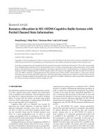
Figure 2: Results of the different methods for subcategories when
the k is changed from 1 to 35 in k-NN query.

test using GMMs gives 0.5% precision error followed by
Euclidean distance having 1.0% precision error.
The histogram method and the KL divergence between
single Gaussians performed clearly worse than measures
based on GMMs. However, the Mahalanobis distance also
gave competitive results. Since the cross-likelihood ratio test
(empirical KL divergence) provided the best results, we can
assume that the original samples contain information which
is not included to GMMs.
Table 2 also illustrates the computational time of a single
distance calculation for each measure. Euclidean distance is
over 10 times faster than Golberger’s approximation, which
is the second fastest measure of those which use multiple
Gaussian components. Considering that Euclidean distance
also provides one of the lowest precision errors makes

it suitable for practical applications. However, it should
be noted that different distance measures require varying
amount of offline preprocessing, for example, generating
different kinds of signal models and histograms. Also, the
further optimization of algorithms might slightly accelerate
some of the measures.
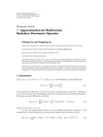
Figure 2 presents the precision of k-NN query for
different methods when k was varied from 1 to 35. The larger
the area below the curve, the better the method is. Here we
can see that the cross-likelihood ratio test using GMMs gave
the best results, followed closely by Euclidean distance and
Mahalanobis distance.
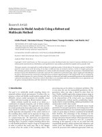
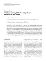
Figure 3 illustrates precision and recall when is changed
in the -range query. Here we can see that in the most parts
of the curve, the cross-likelihood ratio of GMMs gives the
highest precision. However, when a small amount of signals
is retrieved (low recall/high precision) the approximations
of KL divergence, Euclidean distance, and Mahalanobis
distances produces the highest accuracy.


8

EURASIP Journal on Audio, Speech, and Music Processing
1

1

0.9
0.8

0.7

0.95
Precision

Recall

0.6
0.5
0.4

0.9
0.3
0.2
0.1
0

0.85
0

0.1

0.2

0.3

0.4

0.5 0.6
Precision

0.7

0.8

0.9

1

Histogram
Mahalanobis distance
KL-Gaussian
KL-Goldberger
KL-variational
Euclidean distance
GMM cross-likelihood ratio
HMM cross-likelihood ratio

Figure 3: Results of the different methods in -range query for
subcategories when is changed.

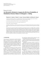
In Figure 4, the distance measures are tested with
different number of GMM components in k-NN query
when k is 10. Generally, the accuracy of all the methods
increases when the number of components is increased.
However, after 12 GMM components there is no significant
change. Thus, 12-component GMMs are used in our other
simulations. Pampalk [40] used cross-likelihood ratio test in
music similarity and the results using 1-component GMMs
were similar to those using 30 components.

Table 3 is a confusion matrix of the query by example
when the Euclidean distance was used and 10 nearest samples
were retrieved. The values in the matrix are the percentage
of the signals retrieved from each category (rows) when the
example was from the certain category (columns). The most
confusion was between the music subcategories, especially
with jazz and popular music. However, these categories were
close to each other also from the human perspective. On
the other hand, the speakers were separated from each other
almost perfectly. The confusion matrix is here presented only
for Euclidean distance, but for other methods the matrices
are rather similar.

5. Discussion
The above results show that the proposed similarity measures
perform well in query by example with the database. The
good performance is partly exampled by the good quality
of the database: the signals within a class are usually
significantly different from those in other classes, and they
do not contain acoustic interference which would make the
problem harder.

0

2

4

6
8

10
12
Number of GMM components

14

16

Euclidean distance
KL-Goldberger
KL-variational
Cross-likelihood ratio test

Figure 4: Results of the Euclidean distance of pdfs for subcategories
when the number of GMM components is changed in k-NN query.

Even though the methods are intended for generic
audio similarity, it is likely that as such they are restricted
only to relatively low-level similarities. For example, it is
very unlikely that the measure will be able to measure
the similarity of speech samples by their topic. This is
naturally affected by the features. In our study the features
measure mostly the spectral characteristics of the signals,
and therefore the methods are able to find spectrally similar
signals, for example samples from the same speaker or the
same musical instrument. It is also likely that the measures
will be affected by the recording setup which affects the
spectral characteristics.
A single audio recording may contain different sound
sources. Depending on the situation, a human can interpret

the mixture consisting of several sources as a whole or
as separate sound sources. For example, in music all the
instruments contribute to the rhythm and harmonicity, but
one can also concentrate to and identify single instruments.
Furthermore, a long recording can consist of sequential
entities which differ significantly from each other. In practice
this requires processing a recording in smaller entities. For
example, Eronen et al. [41] segmented the input signal and
applied supervised classification on each segment.
For practical applications, the speed of operations is an
essential factor. The computational complexity of proposed
methods is relatively low. The distance calculation between
two 10-second samples, depending on the measure, takes
from 0.87 ms (Euclidean distance) to 510 ms (Monte Carlo
approximation of KL divergence) with the tested GMM
distances. The algorithms were implemented with Matlab
and simulations were made with 3.0 GHz PC. The estimation
of GMM or HMM parameters is also time consuming, but
the model need to be estimated only once for each sample.


0

0.2

0.1

0

0

0

0

0

0

0

0

0

0.2

0

0

0

Road

Jazz

Drums

Popular

Classical

Humming

Singing

Whistling

Speaker1

Speaker2

Speaker3

Speaker4

Speaker5

Speaker6

Speaker7

99.5

In a restaurant

Inside a car

0

0

0

0

0

0

0

0

0

0

0

0

0

0

0

98.8

1.2

0

0

0

0

0

0

0

0

0

0

0

0.3

0

0

92.4

2.6

4.7

0

0

0

0

0

0

0

0.1

0.2

0.4

0.5

8.4

0

90.2

0

0

0

4.5

0

0

0

0

0

0

0.7

1.1

0

0

0.2

93.6

0

0

0

0

0

0

0

0

0

0

0

0

0

0

0.5

87.8

0.1

11.6

0

0

0

0.4

0

0

0

0

0

0.8

0.4

0.4

0.6

78.0

13.5

0

5.9

0

0

0

0

0

0.3

0

0

0

0.4

0

3.7

90.8

0

0

0

0.2

0

0

0

0

0

1.8

0

0

0

0

0.5

93.5

4.0

0

0.2

0

0.2

0

0

0

1.3

0

0

0

0

0

0

97.9

0.4

0.5

0.4

0.9

0

0.4

0

0

0

0

0

0

0

0

0

100

0

0

0

0

0

0

0

0

0

0

0

0

0

0

0.1

99.9

0

0

0

0

0

0

0

0

0

0

0

0

0.2

0

0

97.7

2.1

0

0

0

0

0

0

0

0

0

0

0

0

0

0

100

0

0

0

0

0

0

0

0

0

0

0

0

0

0

0

100

0

0

0

0

0

0

0

0

0

0

0

0

0

0

0

99.7

0

0

0.3

0

0

0

0

0

0

0

0

0

0

0

0

100

0

0

0

0

0

0

0

0

0

0

0

0

0

0

0

0

Inside a car In a restaurant Road Jazz Drums Popular Classical Humming Singing Whistling Speaker1 Speaker2 Speaker3 Speaker4 Speaker5 Speaker6 Speaker7

Table 3: Confusion matrix for Euclidean distance when 10 nearest neighbors were retrieved. The values in the matrix are the percentage of the signals retrieved from each category (rows)
when the example was from the certain category (columns).

EURASIP Journal on Audio, Speech, and Music Processing
9


10

EURASIP Journal on Audio, Speech, and Music Processing

When a search is performed in a very large database, it
becomes exhaustive to go through the whole database and to
calculate the distance between the example and all database
samples. One solution proposed to solve this problem is
clustering the database prior the search. In the search phase
it is then possible to restrict the search only to a few clusters
[42].
The way the GMMs are trained has an effect on the
accuracy of the similarity estimation. We also tested Parzenwindow [43, pages 164–174] approach which assigns a GMM
component with fixed variance for each observation so that
I equals the number of frames, µi is the feature vector
within frame i, Σi is fixed, and wi = 1/I. However, the
results were quite similar with the EM algorithm and the
Parzen window method is not very practical since the computational complexity is very high compared to the GMMs

obtained with the EM algorithm. Euclidean distance was
also calculated between full-covariance GMMs. However, the
results of diagonal covariance algorithm were clearly better.
A major problem with full-covariance GMMs is that within
a short signal (430 frames in our simulations) the features
often exhibit multicollinearity and therefore the covariances
become easily singular, making robust estimation of full
covariance matrices difficult.

The term which is the sum of two quadratic forms can be
written as the sum of a single quadratic form and a scalar
(see also [44, 45]) by
x − µA

T

−
Σ A 1 x − µA + x − µB

T

= x − µC

−
Σ B 1 x − µB

(A.2)
−1

ΣC x − µC + q,

where
−
−
−
ΣC 1 = ΣA 1 + ΣB 1 ,

(A.3)

−
−
µC = ΣC ΣA 1 µA + ΣB 1 µB ,

(A.4)

−
−
−
q = µ T Σ A 1 µ A + µT Σ B 1 µ B − µ T Σ C 1 µ C .
A
B
C

(A.5)

Thus, we can write the integral of (A.1) as
∞
−∞

N x; µA , ΣA N x; µB , ΣB dx

=

∞
−∞ (2π)

6. Conclusions

N

1
|ΣA ||ΣB |

× exp −

This paper proposed a query by example system for generic
audio. We measure the similarity between two audio samples
by the distance of the pdfs of their frame-wise feature
vectors. Based on the simulation results, we conclude that
the distance between pdfs can be used as an accurate
similarity estimate for audio signals. Estimating the pdfs of
continuous-valued features cannot be done exactly, but the
use of GMMs or HMMs turned out to be a good solution.
The simulations revealed that the the cross-likelihood
ratio test between GMMs and Euclidean distance gave the
most accurate results in query by example. From the methods
based on simpler statistics, the Mahalanobis distance gave
quite competitive results. However, none of the tested
methods gave clearly the best results and thus the similarity
measure should be chosen according to the application at

hand.

T

=

1
x − µC
2

T

−
ΣC 1 x àC

q
dx
2

q
(2)N/2 |C |
exp
2
(2)N |A ||B |
ì



1

(2)

N/2

|C |

exp −

1
x − µC
2

T

−
Σ C 1 x − µC

dx.
(A.6)

Since the last integrand in (A.6) is a multivariate normal
density which integrates to unity, then we get
∞
−∞

N x; µA , ΣA N x; µB , ΣB dx
=

|ΣC |

(2π)N/2

q
exp − .
2
|ΣA ||ΣB |

(A.7)

Appendix
By substituting (A.3) back to the above equation, it simplifies
to

Integrating the Product of Two
Normal Distributions

∞

The product of two normal distributions can be written as

−∞

N x; µA , ΣA N x; µB , B
=

(2)N

=

1

|A ||B |

1
ì exp
2

T

N x; àA , A N x; µB , ΣB dx

T

−
−
x − µA Σ A 1 x − µA + x − µB Σ B 1 x − µ B

.

(A.1)

(2π)N/2

q
1
exp − .
2
|ΣA + ΣB |

(A.8)

The above equation in combination with (A.3), (A.4), and
(A.5) that can be used to obtain q gives the closed-form
solution for the integral over the product of two normal
distributions.


EURASIP Journal on Audio, Speech, and Music Processing

11

References
[1] J. Song, S.-Y. Bae, and K. Yoon, “Query by humming: matching
humming query to polyphonic audio,” in Proceedings of the
IEEE International Conference on Multimedia and Expo (ICME
’02), pp. 329–332, Lausanne, Switzerland, August 2002.
[2] L. Lu, H. You, and H.-J. Zhang, “A new approach to query
by humming in music retrieval,” in Proceedings of the IEEE
International Conference on Multimedia and Expo (ICME ’01),
pp. 595–598, Tokyo, Japan, August 2001.
[3] A. Kapur, M. Benning, and G. Tzanetakis, “Query-by-beatboxing: music retrieval for the DJ,” in Proceedings of the
15th International Conference on Music Information Retrieval
(ISMIR ’04), Barcelona, Spain, October 2004.
[4] S.-Y. Kung and J.-N. Hwang, “Neural networks for intelligent
multimedia processing,” Proceedings of the IEEE, vol. 86, no. 6,
pp. 1244–1271, 1998.
[5] A. Pikrakis, S. Theodoridis, and D. Kamarotos, “Classification
of musical patterns using variable duration hidden Markov
models,” IEEE Transactions on Audio, Speech and Language
Processing, vol. 14, no. 5, pp. 1795–1807, 2006.
[6] M. Hel´ n and T. Lahti, “Query by example methods for audio

e
signals,” in Proceedings of the 7th Nordic Signal Processing
Symposium (NORSIG ’06), pp. 302–305, Reykjavik, Iceland,
June 2006.
[7] M. Hel´ n and T. Virtanen, “Query by example of audio
e
signals using Euclidean distance between Gaussian mixture
models,” in Proceedings of the IEEE International Conference on
Acoustics, Speech and Signal Processing (ICASSP ’07), vol. 1, pp.
225–228, Honolulu, Hawaii, USA, April 2007.
[8] S. Kiranyaz, A. F. Qureshi, and M. Gabbouj, “A generic audio
classification and segmentation approach for multimedia
indexing and retrieval,” IEEE Transactions on Audio, Speech
and Language Processing, vol. 14, no. 3, pp. 1062–1081, 2006.
[9] J. Assfalg, A. Del Bimbo, and P. Pala, “Image retrieval
by positive and negative examples,” in Proceedings of the
International Conference on Pattern Recognition (ICPR ’00),
vol. 15, pp. 267–270, Barcelona, Spain, September 2000.
[10] G. Aggarwal, P. Dubey, S. Ghosal, A. Kulshreshtha, and
A. Sarkar, “iPURE: perceptual and user-friendly retrieval of
images,” in Proceedings of IEEE International Conference on
Multi-Media and Expo (ICME ’00), pp. 693–696, New York,
NY, USA, July-August 2000.
[11] J.-J. Aucouturier and F. Pachet, “Improving timbre similarity:
how high is the sky?” Journal of Negative Results in Speech and
Audio Sciences, vol. 1, no. 1, pp. 1–13, 2004.
[12] E. Zwicker and H. Fastl, Psychoacoustics: Facts and Models,
Springer, Berlin, Germany, 1999.
[13] M. Mandel and D. Ellis, “Song-level features and support
vector machines for music classification,” in Proceedings of the

6th International Conference on Music Information Retrieval
(ISMIR ’05), London, UK, September 2005.
[14] J. J. Burred and A. Lerch, “A hierarchical approach to
automatic musical genre classification,” in Proceedings of the
6th Conference on Digital Audio Effects (DAFx ’03), London,
UK, September 2003.
[15] C. Uhle, C. Dittmar, and T. Sporer, “Extraction of drum
tracks from polyphonic music using independent subspace
analysis,” in Proceedings of the 4th International Symposium on
Independent Component Analysis and Blind Signal Separation
(ICA ’03), Nara, Japan, April 2003.
[16] T. Stadelmann and B. Freisleben, “Fast and robust speaker
clustering using the earth mover’s distance and Mixmax

[17]

[18]

[19]

[20]

[21]

[22]

[23]

[24]

[25]

[26]

[27]

[28]

[29]

models,” in Proceedings of the IEEE International Conference on
Acoustics, Speech and Signal Processing (ICASSP ’06), vol. 1, pp.
989–992, Toulouse, France, May 2006.
S. Meignier, J. Bonastre, and I. Magrin-Chagnolleau, “Speaker
utterances tying among speaker segmented audio documents
using hierarchical classification: towards speaker indexing
of audio databases,” in Proceedings of the 7th International
Conference on Spoken Language Processing (ICSLP ’02), pp.
577–580, Denver, Colo, USA, September 2002.
T. Virtanen and M. Hel´ n, “Probabilistic model based simie
larity measures for audio query-by-example,” in Proceedings of
the IEEE Workshop on Applications of Signal Processing to Audio
and Acoustics (WASPAA ’07), pp. 82–85, New Paltz, NY, USA,
October 2007.
B. Zhou and J. H. L. Hansen, “Unsupervised audio stream
segmentation and clustering via the Bayesian information
criterion,” in Proceedings of the International Conference on
Spoken Language Processing (ICSLP ’00), vol. 3, pp. 714–717,
Beijing, China, October 2000.
S. Chen and P. Gopalakrishnan, “Speaker, environment and

channel change detection and clustering via the Bayesian
information criterion,” in Proceedings of the Broadcast News
Transcription and Understanding Workshop (DARPA ’98),
Lansdowne, Va, USA, February 1998.
K. Kashino, T. Kurozumi, and H. Murase, “A quick search
method for audio and video signals based on histogram
pruning,” IEEE Transactions on Multimedia, vol. 5, no. 3, pp.
348–357, 2003.
Y. Linde, A. Buzo, and R. Gray, “An algorithm for vector
quantizer design,” IEEE Transactions on Communications
Systems, vol. 28, no. 1, pp. 84–95, 1980.
H. Ferhatosmanoglu, E. Tuncel, D. Agrawal, and A. El Abbadi,
“Approximate nearest neighbor searching in multimedia
databases,” in Proceedings of the 17th IEEE International
Conference on Data Engineering (ICDE ’01), pp. 503–511,
Heidelberg, Germany, April 2001.
A. P. Dempster, N. M. Laird, and D. B. B. Rubin, “Maximum
likelihood from incomplete data via the EM algorithm,”
Journal of the Royal Statistical Society B, vol. 39, no. 1, pp. 1–38,
1977.
J. Goldberger, S. Gordon, and H. Greenspan, “An efficient
image similarity measure based on approximations of KLdivergence between two Gaussian mixtures,” in Proceedings
of the 9th IEEE International Conference on Computer Vision
(ICCV ’03), vol. 1, pp. 487–493, Nice, France, October 2003.
J. R. Hershey and P. A. Olsen, “Approximating the Kullback
Leibler divergence between Gaussian mixture models,” in
Proceedings of the IEEE International Conference on Acoustics,
Speech and Signal Processing (ICASSP ’07), vol. 4, pp. 317–320,
Honolulu, Hawaii, USA, April 2007.
D. A. Reynolds, E. Singer, B. A. Carlson, G. C. O’Leary, J. J.

McLaughlin, and M. A. Zissman, “Blind clustering of speech
utterances based on speaker and language characteristics,”
in Proceedings of the 5th International Conference on Spoken
Language Processing (ICSLP ’98), pp. 3193–3196, Sydney,
Australia, December 1998.
A. Solomonoff, A. Mielke, M. Schmidt, and H. Gish, “Clustering speakers by their voices,” in Proceedings of IEEE International Conference on Acoustics, Speech, and Signal Processing
(ICASSP ’98), vol. 2, pp. 757–760, Seattle, Wash, USA, May
1998.
J. Yin and Q. Yang, “Integrating hidden Markov models
and spectral analysis for sensory time series clustering,” in


12

[30]

[31]

[32]

[33]

[34]

[35]

[36]

[37]

[38]

[39]

[40]

[41]

[42]

[43]
[44]

EURASIP Journal on Audio, Speech, and Music Processing
Proceedings of the IEEE International Conference on Data Mining (ICDM ’05), pp. 506–513, Houston, Tex, USA, November
2005.
J.-J. Aucouturier, Ten experiments on the modelling of polyphonic timbre, Ph.D. dissertation, University of Paris, Paris,
France, 2006.
L. E. Baum, T. Petrie, G. Soules, and N. Weiss, “A maximization technique occuring in the statistical analysis of
probabilistic functions of Markov chains,” The Annals of
Mathematical Statistics, vol. 41, no. 1, pp. 164–171, 1970.
K. Laurila, “Noise robust speech recognition with state
duration constraints,” in Proceedings of the IEEE International
Conference on Acoustics, Speech and Signal Processing (ICASSP
’97), vol. 2, pp. 871–874, Munich, Germany, April 1997.
J. R. Hershey and P. A. Olsen, “Variational Bhattacharyya
divergence for hidden Markov models,” in Proceedings of the
IEEE International Conference on Acoustics, Speech and Signal
Processing (ICASSP ’08), pp. 4557–4560, Las Vegas, Nev, USA,
March 2008.

V. Peltonen, J. Tuomi, A. Klapuri, J. Huopaniemi, and T. Sorsa,
“Computational auditory scene recognition,” in Proceedings
of the IEEE International Conference on Acoustics, Speech and
Signal Processing (ICASSP ’02), vol. 2, pp. 1941–1944, Orlando,
Fla, USA, May 2002.
J. Paulus and T. Virtanen, “Drum transcription with nonnegative spectrogram factorisation,” in Proceedings of the
13th European Signal Processing Conference (EUSIPCO ’05),
Antalya, Turkey, September 2005.
M. Goto, H. Hashiguchi, T. Nishimura, and R. Oka, “RWC
music database: popular, classical, and jazz music databases,”
in Proceedings of the 3rd International Conference on Music
Information Retrieval (ISMIR ’02), Paris, France, October
2002.
T. Viitaniemi, A. Klapuri, and A. Eronen, “A probabilistic
model for the transcription of single-voice melodies,” in Proceedings of the Finnish Signal Processing Symposium (FINSIG
’03), pp. 59–63, Tampere, Finland, May 2003.
J. Kominek and A. Black, “The CMU ARCTIC speech
databases,” in Proceedings of the 5th ISCA Speech Synthesis
Workshop (SSW ’04), pp. 223–224, Pittsburgh, Pa, USA, June
2004.
M. M. Rahman, P. Bhattacharya, and B. C. Desai, “Similarity
searching in image retrieval with statistical distance measures
and supervised learning,” in Proceedings of the 3rd International Conference on Advances in Pattern Recognition (ICAPR
’05), vol. 3686 of Lecture Notes in Computer Science, pp. 315–
324, Bath, UK, August 2005.
E. Pampalk, Computational models of music similarity and their
applications in music information retrieval, Ph.D. dissertation,
Technische Universitat, Wien, Austria, 2006.
A. J. Eronen, V. T. Peltonen, J. T. Tuomi, et al., “Audio-based
context recognition,” IEEE Transactions on Audio, Speech and

Language Processing, vol. 14, no. 1, pp. 321–329, 2006.
M. Hel´ n and T. Lahti, “Query by example in large databases
e
using key-sample distance transformation and clustering,”
in Proceedings of the 3rd IEEE International Workshop on
Multimedia Information Processing and Retrieval (MIPR ’07),
pp. 303–308, Taichung, Taiwan, December 2007.
R. O. Duda, P. E. Hart, and D. G. Stork, Pattern Classification,
John Wiley & Sons, New York, NY, USA, 2nd edition, 2001.
P. Ahrendt, “The multivariate Gaussian probability distribution,” Tech. Rep., IMM, Technical University of Denmark,
Bygning, Denmark, January 2005.

[45] M. J. F. Gales and S. S. Airey, “Product of Gaussians for speech
recognition,” Computer Speech and Language, vol. 20, no. 1,
pp. 22–40, 2006.