báo cáo hóa học:" Research Article A Variable Step-Size Proportionate Affine Projection Algorithm for Identification of Sparse Impulse Response" pot

Hindawi Publishing Corporation
EURASIP Journal on Advances in Signal Processing
Volume 2009, Article ID 150914, 10 pages
doi:10.1155/2009/150914
Research Article
A Variable Step-Size Proportionate Affine Projection Algorithm
for Identification of Sparse Impulse Response
Ligang Liu,
1, 2
Masahiro Fukumoto,
1
Sachio Saiki,
1
and Shiyong Zhang
2
1
Department of Information Systems Engineering, Kochi University of Technology, 185 Miyanokuchi, Kochi 782-8502, Japan
2
School of Computer Science, Fudan University, 220 Handan Road, Shang hai 200433, China
Correspondence should be addressed to Masahiro Fukumoto,
Received 13 January 2009; Revised 19 May 2009; Accepted 5 August 2009
Recommended by Jose Carlos Bermudez
Proportionate adaptive algorithms have been proposed recently to accelerate convergence for the identification of sparse impulse
response. When the excitation signal is colored, especially the speech, the convergence performance of proportionate NLMS
algorithms demonstrate slow convergence speed. The proportionate affine projection algorithm (PAPA) is expected to solve this
problem by using more information in the input signals. However, its steady-state performance is limited by the constant step-size
parameter. In this article we propose a variable step-size PAPA by canceling the a posteriori estimation error. This can result in high
convergence speed using a large step size when the identification error is large, and can then considerably decrease the steady-state
misalignment using a small step size after the adaptive filter has converged. Simulation results show that the proposed approach
can greatly improve the steady-state misalignment without sacrificing the fast convergence of PAPA.
Copyright © 2009 Ligang Liu et al. This is an open access article distributed under the Creative Commons Attribution License,

which permits unrestricted use, distribution, and reproduction in any medium, provided the original work is properly cited.
1. Introduction
Adaptive filtering algorithms can find application in many
real-world systems [1–3], such as wireless channel equalizers,
echo cancelers, noise reduction, and speech enhancement,
for example, an echo canceler is designed to identify an
unknown echo path. Its output is a replica of the echo signal,
which is then removed from the near-end signal to achieve
echo cancellation. Nowadays, echo path is becoming longer
and longer with the increased demand for higher-quality
communication, especially for voice-over IP systems. For
a network echo canceler, the number of coefficients varies
from 512 to 2048 in order to deal with a total delay greater
than 64 milliseconds [4]. Conventional adaptive algorithms,
such as the least mean square (LMS) algorithm and the
normalized LMS (NLMS) algorithm [2, 5], suffer severely
from slow convergence with this kind of long filter, especially
for colored signals. Much effort has been made to design new
algorithms to improve the convergence speed of adaptive
filters with hundreds or thousands of coefficients.
A new kind of proportionate adaptive filtering algorithm
has received much attention recently [6–8]. Proportionate
adaptive algorithms are based on the fact that most long
impulse responses are sparse in nature because only a small
percentage of coefficients are active and most of the others
are zeros. Conventional adaptive algorithms assign the same
step size to all coefficients. As a result, large coefficients
require many more iterations to converge than small ones.
To accelerate the convergence of the large coefficient, it
seems that we should assign them larger step size than that

of small ones, which will yield proportionate adaptation.
The idea behind proportionate adaptive algorithms is to
update each coefficient of the filter individually by assigning
each coefficient a step size proportionate to its estimated
magnitude. Various proportionate adaptive algorithms have
been proposed to exploit this sparse structure. Their con-
vergence speeds are greatly improved [7] over conventional
adaptive algorithms. The proportionate NLMS (PNLMS)
algorithm was firstly proposed in [9]. It greatly speeds
up the initial convergence of adaptive filters. However, its
convergence begins to slow dramatically thereafter. Many
modifications have been proposed to improve it, such as the
PNLMS++ algorithm [10], the IPNLMS algorithm [11], the
CPNLMS algorithm [12], the improved IPNLMS algorithm
[13], the IPMDF algorithm [14], and the mu-law PNLMS
(MPNLMS) algorithm [15]. Among these variants, the
2 EURASIP Journal on Advances in Signal Processing
MPNLMS algorithm is one of the fastest in the framework
of proportionate adaptation. Instead of using magnitude
directly, the logarithm of the magnitude is used as the step
gain of each coefficient, so the MPNLMS algorithm can
consistently converge to the steady state for sparse impulse
response. The SPNLMS algorithm [15] is proposed to reduce
the heavy computational complexity of MPNLMS without
loss of fast convergence.
The step-size control matrix of MPNLMS was derived
on the assumption that the input is white. For colored input
signals, especially speech, convergence speed will depend on
the eigenvalues of the input signal’s autocorrelation matrix.
The proportionate affine projection algorithm (PAPA) is the

natural extension of the PNLMS algorithm. It is expected to
present faster convergence for highly correlated input signals
at the cost of a modest increase in computational complexity.
Besides convergence speed, another important aspect of
the adaptive algorithm is its steady-state performance: low
misalignment is desirable. Unfortunately, the design of the
step-size control matrix cannot decrease the misalignment in
the framework of proportionate adaptation. The steady-state
misalignment of the proportionate algorithms is approxi-
mately equal to that of their nonproportionate counterparts
[9]. We know that the step-size parameter reflects a tradeoff
between fast convergence and low misalignment. When step
size is adjusted to obtain faster convergence, misalignment
becomeslarger,andviceversa.Ifweadaptivelycontrol
the step size to be large in the transient state and to be
small as convergence proceeds, both fast convergence and
low misalignment can be achieved. Different adaptive step-
size control approaches have been proposed and studied
in literature relating to this concept. In [16], the squared
instantaneous error was exploited as a criterion to change
the step size. In [17], an optimal step size was proposed for
NLMS algorithm by minimizing the mean-square deviation
at each iteration. A variable step-size NLMS algorithm was
described in [18] to improve the estimation of the power level
of the disturbance signals. It was used to decide the optimal
step size at each iteration. In [19], a steepest descent method
was proposed to adaptively update the step size to minimize
squared error. By combining the input vector and the
instantaneous error vector, a variable step-size approach was
proposed for APA in [20]. A nonparametric variable step-size

NLMS algorithm, NPVSS-NLMS, was proposed in [21]by
adjusting the step size to cancel a posteriori error. Recently,
this approach was applied in the undermodeling acoustic
echo cancellation system [22, 23]. It was further extended
to APA with a new perspective of signal enhancement in
[24]. As can be seen, these approaches are only applicable to
nonproportionate adaptive algorithms.
In this article, we propose a variable step-size pro-
portionate affine projection algorithm (VSS-PAPA) for the
identification of sparse impulse response. Theoretically, in
a noise free environment, PAPA has optimal convergence
speed and zero misalignment by canceling the a posteriori
output estimation error at each iteration. However, with the
presence of a disturbance signal, canceling the a posteriori
estimation error will introduce additional noise into the
coefficient update [21]. Taking the effect of background
noise into account, we derive a PAPA with variable step
size parameter to cancel a posteriori estimation error at
each iteration. The variable step size is large when the
adaptive filter is in its transient state. Hence, it converges
fast. Then the step size becomes small when the adaptive
filter reaches the steady state, so misalignment is significantly
decreased. The proposed algorithm demonstrates excellent
performance by combining the fast proportionate algorithm
with variable step-size technique for identification of sparse
impulse response.
The organization of this article is as follows. In Section 2,
we briefly overview the proportionate affine projection
algorithm and various definitions of the step-size control
matrix of proportionate adaptation. In Section 3,avariable

step size approach is proposed for PAPA to achieve bet-
ter performance. In Section 4, many computer simulation
results are presented to illustrate the excellent performance
of the proposed algorithm. Finally, Section 5 concludes our
research.
2. Overview of Proportionate
Adaptive Algorithms
Consider a system identification problem. Bold lowercase
letters indicate vectors and bold uppercase letters denote
matrices. All vectors are column vectors, (
·)
T
indicates
transpose, and t is the time index. Also, w
opt
is an unknown
sparse impulse response and w is an adaptive filter. The
length of w
opt
and w is supposed to be same, N. The input
vector x(t)
= [x(t) x(t −1) x(t −N +1)]
T
, the output of
the adaptive filter y(t)
= w
T
opt
x(t), and the desired signal
d(t)

= y(t)+v(t), where v(t) is a disturbance signal, which
may be background noise or/and measurement noise.
The APA achieves a faster convergence speed for cor-
related input signals than the NLMS algorithm with only
a modest increase in computational complexity. It exploits
more information from the input signal, not only the current
input vector but also the most recent P input vectors. The
proportionate APA (PAPA) is expected to converge faster
than the proportionate NLMS algorithms for colored input
signals. Define P as the projection order, the input matrix as
the P successive input vector, X(t)
= [x(t) x(t − 1) x(t −
P + 1)], and the desired vector as the P successive past value
of d(t), d(t)
= [d(t) d(t −1) ···d(t −P +1)]
T
. The error
vector e(t)canbewrittenas
e
(
t
)
= d
(
t
)
−X
T
(
t

)
w
(
t
)
. (1)
The PAPA can be briefly summarized as follows:
w
(
t +1
)
= w
(
t
)
+ αG
(
t
)
X
(
t
)

X
T
(
t
)
G

(
t
)
X
(
t
)
+ εI

−1
e
(
t
)
,
(2)
G
(
t
)
= diag

g
0
(
t
)
, g
1
(

t
)
, , g
N−1
(
t
)

,
(3)
EURASIP Journal on Advances in Signal Processing 3
where α is a overall constant step size,
 is the regularization
parameter, and I is a P
×P identity matrix. The definition of
the diagonal element of matrix G(t) can be summarized as
L
max
= max

δ
ρ
, F
(
w
0
(
t
))
, , F

(
w
N−1
(
t
))

,(4)
γ
n
(
t
)
= max

F
(
w
n
(
t
))
, ρL
max

,(5)
g
n
(
t

)
=
γ
n
(
t
)
(
1/N
)

N−1
i
=0
(
t
)
.
(6)
Here, F is a real-valued function to map the current
coefficient estimate into a certain value of the proportionate
step-size parameter; δ
ρ
is used to prevent w(t) from stalling
at the beginning, and has a typical value of 0.01; ρ is used
to prevent the very small coefficients from stalling, and
has typical values in the range from 1/N to 5/N [9]. Note
that when P
= 1, the PAPA degenerates into the PNLMS
algorithm, and when all of the elements of G(t)areidentical,

that is, g
0
(t) =···=g
N−1
(t) = 1, the PAPA reduces to the
standard APA.
The PNLMS algorithm [9] has proposed a simple
function as F(w
n
(t)) =|w
n
(t)|. It has very fast initial con-
vergence speed. However, its convergence slows thereafter.
Furthermore, its convergence speed degrades greatly if the
target impulse response is not sparse enough. The MPNLMS
algorithm proposed in [15, 25] achieves the fastest step size
control matrix G(t) in the proportionate adaptation frame-
work. Instead of using the absolute value of the coefficient
magnitude directly, its logarithm is used as the step size.
Hence, both large and small coefficients converge at the same
rate, so that the overall convergence speed of the adaptive
filter is greatly accelerated. For MPNLMS, F(w
n
(t)) = ln(1 +
μ
|w
n
(t)|), where μ is an objective convergence criterion,
typically μ
= 1000. Many simulation results have proved that

the MPNLMS algorithm is one of the fastest proportionate
algorithms [26]. The main disadvantage of MPNLMS is
its heavy computation cost because of the presence of N
logarithmic operations in every iteration. A line segment is
proposed to approximate the mu-law function, which leads
to a computation efficient algorithm, SPNLMS [25], where
F
(
w
n
(
t
))
=
⎧
⎨
⎩
400|w
n
(
t
)
|, |w
n
(
t
)
| < 0.005,
2, otherwise.
(7)

The step-size control matrix defined by MPNLMS was
derived on the assumption that the input is white. The mu-
law PAPA (MPAPA) is expected to achieve faster convergence
speed than MPNLMS for colored input signals. Its compu-
tation efficient version, SPAPA, is favorable for real-world
application because of its implementable low computational
complexity.
3. Variable Step-Size Proportionate Affine
Projection Algorithms
3.1. Algorithm Formulation. Our objective is to find a
variable step-size approach that is applicable to PAPAs.
Unfortunately, because of the presence of G(t), it is very
difficult to analyze the transient performance of PAPAs. In
thissection,weproposeavariablestepsizeforPAPA.
The APA can be derived from the principle of least
perturbation, that is, to maintain the next coefficient vector
as close as possible to the current estimate, while forcing the a
posteriori output estimation error to be zeros [2, 5, 27]. The
a posteriori output estimation error vector r(t)isdefinedas
[5]
r
(
t
)
= d
(
t
)
−X
T

(
t
)
w
(
t +1
)
= X
T
(
t
)
w
(
t +1
)
+ v
(
t
)
,
w
(
t
)
= w
opt
−w
(
t

)
,
(8)
where
w(t) is the coefficient error vector and v(t) =
[v(t) v(t −1) ···v(t −P +1)]
T
is the disturbance signal
vector. Compared to r(t), the error e(t)in(1) plays the role
of the a priori output estimation error vector.
The APA can satisfy the principle of least perturbation
in a noise-free system. It has the fastest convergence speed
and zero misalignment by canceling r(t)ateachiteration.
The optimal step size is one in this case. However, in practical
application, a disturbance signal is inevitable. Therefore, the
adaptive algorithm cannot achieve zero misalignment. This
could be explained by the fact that in the presence of v(t),
attempts to force r(t) to be zero will introduce noise to the
adaptive filter update [21]. Actually, what we would like is to
force the a posteriori estimation error to be zero. That is
X
T
(
t
)
w
(
t +1
)
= 0,(9)

where 0 is a P
×1 column vector whose elements are all zeros.
Combining (8)with(9) implies that in a noisy environment
we should update the coefficients to make the a posteriori
error not to be zero, but to be the disturbance signal: v(t),
r
(
t
)
= v
(
t
)
. (10)
In practical application, although the disturbance signal
v(t) is not available, its power level can be estimated. For this
reason, the optimal step-size parameter can be found in such
a way that
E

r
2
p
(
t
)

=
E


v
2
p
(
t
)

, p = 0 ···P −1, (11)
where r
p
(t) is the pth element of r(t), and v
p
(t) is the pth
element of v(t). Note that v
p
(t) = v(t − p).
Based on above notion, a VSS-PAPA can be derived as
follows. Rewrite (2)withaP
× P time-varying step-size
diagonal matrix α(t), ignoring the regularization term
I,:
w
(
t +1
)
= w
(
t
)
+ G

(
t
)
X
(
t
)

X
T
(
t
)
G
(
t
)
X
(
t
)

−1
α
(
t
)
e
(
t

)
.
(12)
Subtracting w
opt
at both sides and rearranging the terms, we
get
w
(
t +1
)
= w
(
t
)
−G
(
t
)
X
(
t
)

X
T
(
t
)
G

(
t
)
X
(
t
)

−1
α
(
t
)
e
(
t
)
.
(13)
4 EURASIP Journal on Advances in Signal Processing
Premultiplying X
T
(t) at both sides yields a relation between
the a posteriori estimation error and the a priori output
estimation error:
r
p
(
t
)

=

1 − α
p
(
t
)

e
p
(
t
)
, (14)
where α
p
(t) is the pth diagonal element of α(t), and e
p
(t)
is the pth element of e(t). This result is very interesting in
relation to PAPA. It can be observed that the a posteriori
estimation error r(t) is determined by the step size param-
eter α(t)anderrorvectore(t) and is independent from
G(t). Consequently, a simple variable step-size approach is
expected for PAPA from this relation, following a procedure
similar to [24].
Squaring and taking mathematical expectation at both
sides of (14), and combining it with (11), give
E


r
2
p
(
t
)

=

1 − α
p
(
t
)

2
E

e
2
p
(
t
)

=
E

v
2


t − p

. (15)
Solving the equation, the pth time-varying step-size α
p
(t)is
obtained with a simple expression as
α
p
(
t
)
= 1 −




σ
2
v

t − p

σ
2
e
p
(
t

)
, (16)
where σ
2
v
(t −p) = E{v
2
(t −p)} is the variance of v(t −p)and
σ
2
e
p
(t) = E{e
2
p
(t)} is the variance of e
p
(t).
In the transient state of the adaptive filter, σ
2
e
p
(t)will
be large, hence α
p
(t) is also large. Consequently, fast
convergence speed can be expected. After the adaptive filter
reaches to within the immediate vicinity of its optimal value,
σ
2

e
p
(t) becomes small, hence α
p
(t) decreases. As a result, low
misalignment can be observed.
There are some practical considerations related to this
expression. The first is the estimations of σ
2
e
p
(t)andσ
2
v
(t).
The quantity of σ
2
e
p
can be estimated using an exponential
window as
σ
2
e
p
(
t
)
=
(

1
−λ
1
)
σ
2
e
p
(
t
−1
)
+ λ
1
e
2
p
(
t
)
,
(17)
where
λ
1
= 1 −
1
K
1
N

,
(
K
1
∈ Z
+
, K
1
≥ 1
)
. (18)
AlargeK
1
can obtain a smooth estimate of σ
2
e
p
(t)butitwill
reduce the tracking ability of the adaptive filter. In practical
application, power estimation of the disturbance signal,
σ
2
v
(t), can be obtained during the silences in a network echo
cancellation system. An estimate of the disturbance signal,
v(t), can even be obtained using an additional adaptive filter,
as proposed in [18]. Therefore, by using the same method
with
σ
2

e
p
(t), σ
2
v
(t) can be obtained by
σ
2
v
(
t
)
= λ
1
σ
2
v
(
t
−1
)
+
(
1 − λ
1
)
v
2
(
t

)
. (19)
The second issue is stability. These estimates could lead
to minor deviations from their theoretical values, which may
result in a negative step size or a large one and force the
adaptive algorithm to diverge. It is necessary to restrict α
p
(t)
in range so that the stability of the adaptive algorithm is
guaranteed, 0
≤ α
min
≤ α
p
(t) ≤ α
max
≤ 2. Suitable choice
of α
min
and α
max
can make the proposed algorithm robust to
an inaccurate estimate of
σ
2
v
. More detailed discussions on
this issue will be presented in the following subsection.
The third issue is the determination of G(t). Although
it can be determined by any proportionate adaptive algo-

rithm, it is preferable to adopt the segment proportionate
version described in (3)–(6)and(7) because it has excellent
performance and light computation load. We will use this
definition throughout this article. The proposed algorithm
with this definition of G(t) will be referred as VSS-SPAPA for
convenience sake. Note that when G(t) is an identity matrix
the proposed VSS-SPAPA degrades into the VSS-APA in [24].
It seems that the proposed variable step-size PAPA is
similar to the set-membership PAPA (SM-PAPA) proposed
in [28], where α
p
(t) is replaced by
α
sm,p
(
t
)
=
⎧
⎪
⎪
⎨
⎪
⎪
⎩
1 − γ



e

p
(
t
)



,if



e
p
(
t
)



>γ,
0, otherwise.
(20)
Here, γ is a predetermined parameter as a bound on the
noise. Since there is no averaging on, it is obvious that we
cannot expect a lower misalignment than we propose in this
article. The proposed variable step size described in (16)
provides an optimal criteria of γ for the SM-PAPA, that is,
γ should choose according to σ
v
.

3.2. Adaptive Estimate of σ
2
v
(t) and Its Influence. The pro-
posed VSS-SPAPA can obtain optimal α
p
(t)ifanaccurate
estimate of σ
2
v
(t) is available. As explained in the previous
subsection, a relatively accurate estimate can be easily
obtained during silence in a network echo cancellation
system, since there are many pauses in natural speech.
However, if the power of the disturbance signals changes
between two consecutive estimations, its new estimate will
not be available immediately. A method was proposed to
adaptively estimate σ
2
v
(t) only using the signals available in
the system, which can be described by [24]
σ
2
v
(
t
)
= max


0, σ
2
d
(
t
)
− σ
2
y
(
t
)

,
σ
2
d
(
t
)
= λ
2
σ
2
d
(
t
−1
)
+

(
1 − λ
2
)
d
2
(
t
)
,
σ
2
y
(
t
)
= λ
2
σ
2
y
(
t
−1
)
+
(
1 − λ
2
)

y
2
(
t
)
,
(21)
where
y(t) = x
T
(t)w(t) is the output of the adaptive filter,
and
λ
2
= 1 −
1
K
2
N
,
(
K
2
∈ Z
+
, K
2
≥ K
1
)

. (22)
This estimate is approximately accurate after the adaptive
filter has reached its steady state, because
E

v
2
(
t
)

≈
E

d
2
(
t
)

−
E


y
2
(
t
)


. (23)
The method provides a suboptimal solution of σ
2
v
(t)ifitis
unavailable in the given practical application. However, after
EURASIP Journal on Advances in Signal Processing 5
the adaptive filter has converged to within the immediate
vicinity of its optimal value, it can also be found that [22]
E

e
2
(
t
)

≈
E

d
2
(
t
)

−
E



y
2
(
t
)

. (24)
Therefore, the difference between
σ
2
e
p
(t)andσ
2
v
(t)willbe
insignificant in the steady state of the adaptive filter. As
a result, α
p
(t) will be very small, and low steady-state
misalignment observed. However, this approach will lead to
a slow convergence speed if this approach is applied during
the transient period of the adaptive filter, for example, if the
unknown impulse response changes suddenly, this approach
is believed to present poor tracking ability because α
p
(t)
remains relatively small. To improve the adaptive filter’s
tracking ability in this scenario, the value of α
min

should
not be too small, and the steady-state misalignment will be
increased as a consequence. An alternative is to introduce
a impulse response variation detector in the algorithm, see
[24] and reference therein.
Let us discuss the influence of an inaccurate estimate of
σ
2
v
(t) on the convergence performance of the adaptive algo-
rithm. In the case of
σ
2
v
(t)  σ
2
v
(t), α
p
(t) will be smaller than
its optimal value defined in (16). The convergence speed of
the proposed algorithm will be slowed because α
p
(t) reaches
α
min
soon. However, low misalignment will be achieved using
more iterations. In the case of
σ
2

v
(t) = σ
2
v
(t), α
p
(t)willbe
greater than its optimal value. Fast initial convergence speed
will be observed but the misalignment will increase because
α
p
(t) is close to α
max
. For a modest inaccurate estimate of
σ
2
v
(t), the performance of the proposed algorithm is better
than that of the VSS-APA because it benefits from the fast
proportionate adaptive algorithms. The simulation results in
Section 4 show that the proposed algorithm can tolerate a
large
σ
2
v
(t) estimate error.
The proposed variable step-size segment proportionate
affine projection algorithm (VSS-SPAPA) is summarized in
Algorithm 1 .
3.3. Computational Complexity. Compared to the standard

APA, the additional computation load of the proposed VSS-
SPAPA is composed of four parts. First, the calculation of
G(t) costs 2N + 2 multiplications or divisions, N additions,
and 3N comparisons. Second, the calculation of G(t)X(t)
costs PN multiplications. Third, the estimate of
σ
2
e
p
(t)and
calculation of α(t)willcost4P + 6 multiplications or
divisions, P square-root operations, and 2P + 2 additions
or subtractions. Finally, the calculation of α(t)e(t) costs P
multiplication. The remaining operations are common with
APA. In summary, the dominant additional computation
cost of the proposed VSS-SPAPA is (P +2)N +5P +8
multiplications or divisions operations and P square-root
operations. For practical applications, such as network echo
cancellation, the value of projection order P is usually in
the range of 2–8. Therefore, the computational complexity
of the proposed VSS-SPAPA is moderate. We propose that
the additional computation load is worth the considerable
performance improvement in sparse impulse response, and
illustrate this in the following section.
Initialization:
w(0)
= 0; σ
2
v
(0) = 0; σ

2
y
(0) = 0; σ
2
d
(0) = 0;
 = PMσ
2
x
,(M ∈ Z
+
, M ≥ 1)
λ
1
= 1 − 1/(K
1
N), (K
1
∈ Z
+
, K
1
≥ 1)
λ
2
= 1 − 1/(K
2
N), (K
2
∈ Z

+
, K
2
≥ K
1
)
for p
= 0,1, ,P −1
σ
2
e
p
(t) = (1 −λ
1
)σ
2
e
p
(t − 1) + λ
1
e
2
p
(t);
For all t:
g
n
(t) =
⎧
⎨

⎩
400|w
n
(t)|, |w
n
(t)| < 0.005
2, otherwise.
L
max
= max{δ
ρ
, g
0
(t), , g
N−1
(t)}
γ
n
(t) = max{g
n
(t), ρL
max
}
g
n
(t) = γ
n
(t)/[1/N

N−1

i
=0
γ
i
(t)]
G(t)
= diag {g
0
(t), g
1
(t), , g
N−1
(t)}

y(t) = X
T
(t)w(t)
e(t)
= d(t) −y(t)
if
σ
2
v
(t) is not available,
σ
2
d
(t) = λ
2
σ

2
d
(t − 1) + (1 −λ
2
)d
2
(t)
σ
2
y
(t) = λ
2
σ
2
y
(t − 1) + (1 −λ
2
)y
2
(t)
σ
2
v
(t) = max{0, σ
2
d
(t) − σ
2
y
(t)}

for p = 0,1, , P − 1
σ
2
e
p
(t) = (1 −λ
1
)σ
2
e
p
(t − 1) + λ
1
e
2
p
(t)
α
p
(t) = 1 −

σ
2
v
(t − p)/σ
2
e
p
(t)
if α

p
(t) <α
min
, α
p
(t) = α
min
,
if α
p
(t) >α
max
, α
p
(t) = α
max
,
α(t)
= diag {α
0
(t), , α
P−1
(t)}
w(t +1)= w(t)+G(t)X(t)[X
T
(t)G(t)X(t)
+εI]
−1
α(t)e(t)
Algorithm 1: The proposed VSS-SPAPA.

4. Simulation Results
To evaluate the performance of the proposed algorithm,
many computer simulations were conducted in the context
of system identification. Four algorithms are compared in
numerous simulations, APA, SPAPA, VSS-APA [24], and the
proposed VSS-SPAPA. The unknown system w
opt
is taken
from a network echo path illustrated in Figure 1(a).Both
w
opt
and the adaptive filter w have same length, N = 512. For
the proportionate algorithms, δ
ρ
= 0.01, ρ = 1/N. For VSS-
SPAPA, λ
1
= 1 − 1/2N, λ
2
= 1 − 1/4N, α
min
= 0.005. α
max
=
1.0 is assigned because a large step size for SPAPA does
not considerably improve its convergence speed but results
in higher misalignment. The regularization parameters are
chosen by
 = 10Pσ
2

x
for all the algorithms. The disturbance
signal v(t) is an independent white Gaussian noise. The
convergence performance is evaluated using the normalized
misalignment (in dB) defined by
10 log
10
⎛
⎜
⎝



w
opt
−w
(
t
)



2
2



w
opt




2
2
⎞
⎟
⎠
. (25)
4.1. Simulations with Real Value of σ
2
v
(t). We first test the
performance of the proposed VSS-SPAPA with the real value
of σ
2
v
(t). The signal-to-noise rate (SNR) is adjusted to 20 dB
for the simulation results illustrated. The misalignment of
6 EURASIP Journal on Advances in Signal Processing
−0.4
−0.2
0
0.2
0.4
Magnitude
0 102030405060
Time (ms)
(a)
−1
0

1
Magnitude
0 2 4 6 8 101214161820
Time (s)
(b)
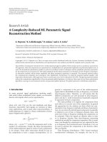
Figure 1: (a) A typical sparse network echo path used in the
simulations. (b) A segment of speech signal with 8 k sampling rate
used in the simulations.
the four algorithms is compared with three kinds of input
signal: (a) white Gaussian noise signal, (b) highly colored
signals generated by an AR(1) process, and (c) speech signals
illustrated in Figure 1(b).
In the first set of simulations, the input sequence was
zero-mean white Gaussian noise signal with σ
2
x
= 1. For
APA and SPAPA, a constant step α
= 1 is assigned.
Figure 2(a) compares convergence speed in the first 15000
iterations of the related algorithms. The projection order
P
= 1. Therefore, the related algorithms degrade into their
corresponding NLMS versions. It can be seen that the
SPNLMS algorithm converges faster than the conventional
NLMS algorithm with same step size. We can also find that
they have almost the same steady-state misalignment. The
proposed VSS-SPNLMS algorithm achieves almost the same
fast initial convergence as the SPNLMS algorithm. However,
it can obtain lower steady-state misalignment; about 18 dB

improvement can be observed in 4
×10
4
iterations, as shown
in Figure 2(b). To achieve this low level misalignment, the
SPNLMS requires a very small step size. However, α is 0.005
in this case, whose convergence speed is greatly degraded.
Although the NPVSS-NLMS algorithm in [21] can achieve
almost the same low misalignment, its convergence speed
is significantly lower than the proposed algorithm. It can
be seen from Figure 2(a) that the proposed VSS-SPNLMS
algorithm reaches
−20 dB misalignment in approximately
900 iterations but the NPVSS-NLMS algorithm reaches that
level in about 2200 iterations. Figure 2(b) illustrates the
results of different projection order. It can be seen that in the
case of white input signal, the increase in the projection order
from 2 to 8 does not considerably improve the convergence
speed of the proposed VSS-SPNLMS. This suggests that
the control matrix G(t) determined by SPNLMS is nearly
optimal for white input signal. The proposed VSS-SPNLMS
is preferred to obtain optimal convergence speed and lower
misalignment with least computation cost.
−30
−25
−20
−15
−10
−5
0

Misalignment (dB)
0 1 2 3 4 5 6 7 8 9 10 11 12 13 14 15
Number of iterations (
×10
3
)
P
= 1
SPNLMS (α
= 1)
NLMS (α
= 1)
Proposed
VSS-SPNLMS
NPVSS-NLMS
(a)
−40
−35
−30
−25
−20
−15
−10
−5
0
Misalignment (dB)
00.511.522.533.54
Number of iterations (
×10
4

)
SPNLMS (α
= 1)
SPNLMS (α
= 0.005)
NPVSS-NLMS
VSS-SPAPA (P
= 1)
VSS-SPAPA (P
= 2)
VSS-SPAPA (P
= 4)
VSS-SPAPA (P
= 8)
(b)
Figure 2: Misalignment of the algorithms with white Gaussian
noise input. (a) P
= 1. (b) Comparison of different projection order,
P
= 1, 2, 4, 8. SPNLMS and NPVSS-NLMS [21] are also illustrated.
In the second set of simulations, the input sequence
{x(t)} is an AR(1) process generated by filtering a zero-
mean white Gaussian signal through a first-order system
G(z)
= 1/(1 −0.9z
−1
). Figure 3(a) illustrates the results with
projection order P
= 2. The proposed VSS-SPAPA achieves
almost the same initial convergence speed with SPAPA,

but it can reach a much lower steady-state misalignment—
approximately 20 dB improvement can be observed in 5
×10
4
iterations. Although VSS-APA can almost achieve this level
of misalignment, its convergence speed is lower than the
proposed VSS-SPAPA. Figure 3(b) shows the misalignment
of the proposed algorithm of different projection order. In
this case, when P
= 1, all of the related algorithms present very
low convergence speed. Their performance can be greatly
improved by increasing P
= 2. However, with the increase in
the projection order from 4 to 8, the convergence speed of
VSS-SPAPA does not increase further, while the convergence
speed of APA and VSS-APA will improve with increased
projection order from 1 to 8. The VSS-SPAPA with P
= 2is
preferable in this case to obtain the best performance with a
modest increase in computational complexity.
EURASIP Journal on Advances in Signal Processing 7
−35
−30
−25
−20
−15
−10
−5
0
Misalignment (dB)

00.511.52 2.533.544.55
Number of iterations (
×10
4
)
P
= 2
SPAPA (α
= 1)
SPAPA (α
= 0.005)
APA (α
= 1)
Proposed
VSS-SPAPA
VSS-APA
(a)
−35
−30
−25
−20
−15
−10
−5
0
Misalignment (dB)
00.511.52 2.533.544.55
Number of iterations (
×10
4

)
SPAPA (P
= 2, α =1)
SPAPA (P
= 2, α = 0.005)
VSS-APA (P
= 2)
VSS-SPAPA (P
= 1)
VSS-SPAPA (P
= 2)
VSS-SPAPA (P
= 4)
VSS-SPAPA (P
= 8)
(b)
Figure 3: Misalignment of the algorithms with highly colored
input generated by G(z). (a) P
= 2. (b) Comparison with different
projection order, P
= 1, 2, 4, 8. SPAPA and VSS-APA are also
illustrated.
In the third set of simulations, the input is from a
speech segment illustrated in Figure 1(b). The disturbance
signal
{v(t)}is uncorrelated zero-mean white Gaussian noise
with SNR
= 20 dB. Figure 4(a) illustrates the result with
projection order P
= 8. The proposed VSS-SPAPA achieves

almost the same fast initial convergence compared to the
SPAPA, but it can achieve lower steady-state misalignment—
-about 15 dB improvement can be observed in 15 seconds. In
this case, VSS-APA cannot achieve this misalignment level
(or it needs many more minutes to achieve it). The VSS-
SPAPA outperforms VSS-APA both on convergence speed
(approximately twice as fast) and on low misalignment
(approximately 2 dB lower). Figure 4(b) compares the con-
vergence of the proposed algorithm at different projection
orders. In the case of speech signal input, with an increase
in projection order from 1 to 8, the convergence speed of
all the related algorithms was improved. Taking into account
computational complexity, the performance of P
= 4 is good
enough in the case of speech signal input with a modest
increase in computation load.
−30
−25
−20
−15
−10
−5
0
Misalignment (dB)
0 1 2 3 4 5 6 7 8 9 10 11 12 13 14 15
Time (s)
P
= 8
SPAPA (α
= 0.005)

SPAPA (α
= 1)
Proposed
VSS-SPAPA
VSS-APA
(a)
−30
−25
−20
−15
−10
−5
0
Misalignment (dB)
0 1 2 3 4 5 6 7 8 9 10 11 12 13 14 15
Time (s)
SPAPA (P
= 8, α = 0.005)
SPAPA (P
= 8, α =1)
VSS-APA (P
= 8)
VSS-SPAPA (P
= 1)
VSS-SPAPA (P
= 2)
VSS-SPAPA (P
= 4)
VSS-SPAPA (P
= 8)

(b)
Figure 4: Misalignment of the algorithms with speech signal. (a)
P
= 8. (b) Comparison with different projection order, P = 1, 2, 4, 8.
SPAPA and VSS-APA are also illustrated.
The tracking ability of the adaptive algorithms is impor-
tant in a nonstationary environment where the unknown
impulse response may suddenly change. In a network
echo cancellation system, the echo path is subject to shift
backward or forward as a result of delay jitter. Figure 5
illustrates the result of the tracking ability of the relevant
algorithms with speech signal input and P
= 4. The unknown
impulse response suddenly shifted to the right by 12 samples.
It can be seen from this figure that the proposed algorithm
presents good tracking performance after the unpredicted
change in the unknown impulse response. Furthermore, it
outperforms its counterparts in low steady-state misalign-
ment after reconvergence.
4.2. Simulations with Inaccurate Estimate of σ
2
v
(t). As dis-
cussed in the previous section, the estimated accuracy of
σ
2
v
(t) influences the convergence of VSS-APA and VSS-
SPAPA. Figure 6 illustrates the simulation results of the
relevant algorithms with AR(1) input signals in subplot (a),

and speech input signals in subplot(b), respectively. We can
8 EURASIP Journal on Advances in Signal Processing
−30
−25
−20
−15
−10
−5
0
5
Misalignment (dB)
0 5 10 15 20 25 30
Time (s)
APA (α
= 0.3)
SPAPA (α
= 0.3)
VSS-APA
VSS-SPAPA
Figure 5: Comparison of tracking ability of the relevant algorithms
with speech signals, P
= 4. The unknown impulse response changes
after 15 seconds.
see that VSS-SPAPA with an accuracy of σ
2
v
(t)isbestamong
the three cases: (1) the power estimate of the disturbance
signal is greater than its real value,
σ

2
v
(t) = 1.5σ
2
v
(t);
(2)
σ
2
v
(t) = σ
2
v
(t); (3) σ
2
v
(t) is smaller than its real value,
σ
2
v
(t) = 0.8σ
2
v
(t). In any case, VSS-SPAPA can maintain fast
convergence with both AR(1) signals and speech signals. In
case (1), a large estimate
σ
2
v
(t)willcauseα

p
(t)tobesmalland
reach α
min
faster than in case (2). In any cases, α
min
warrants
VSS-SPAPA to achieve low misalignment. It is obvious that
this requires more iterations but is still faster than VSS-APA,
as shown in the figure. However, if
σ
2
v
(t) is excessively smaller
than its real value, the steady-state misalignment of VSS-
SPAPA is relatively higher, as shown in the figure, because
α
p
(t) remains large in the steady state—around 0.25 in case
(3). The VSS-SPAPA does not behave worse than the SPAPA
even with a large estimate error of
σ
2
v
(t). It can tolerate more
than +50% estimate error and about
−20% estimate error
of
σ
2

v
(t). The proposed VSS-SPAPA is robust to a relatively
inaccurate estimate of
σ
2
v
(t).
If an estimate of σ
2
v
(t) is not available in practical
application, it can be adaptively estimated according to
(23). Figure 7 illustrates the results of the proposed VSS-
SPAPA with this estimate method included. As discussed
in the previous section, the problem with this adaptive
estimate method is that the estimate is only effective when
the adaptive filter has converged. Otherwise, the estimate
will be very inaccurate and cause α
p
(t)tobeverysmall.
Hence, the tracking ability of the proposed algorithms will be
considerably worsened. So, the relevant algorithms are tested
on the assumption that the unknown impulse response
suddenly changes by shifting to the right 12 samples.
Figure 7(a) is with the highly colored AR(1) input (P
= 2) and
Figure 7(b) is with speech input signals (P
= 8). For SPAPA
and APA, the constant step size is α
= 0.3, which is suitable

for practical application. It can be seen that VSS-SPAPA
can also quickly track the change in unknown impulse
−40
−35
−30
−25
−20
−15
−10
−5
0
Misalignment (dB)
012345
Number of iterations (
×10
4
)
VSS-SPAPA (1)
VSS-SPAPA (2)
VSS-SPAPA (3)
SPAPA (P
= 2, α = 0.3)
VSS-APA (P
= 2)
(a)
−30
−25
−20
−15
−10

−5
0
Misalignment (dB)
0 5 10 15 20
Time (s)
VSS-SPAPA (1)
VSS-SPAPA (2)
VSS-SPAPA (3)
SPAPA (P
= 8, α = 0.3)VSS-APA (P = 8)
(b)
Figure 6: Misalignment of the relevant algorithms with inaccurate
estimate of
σ
2
v
(t). (a) With highly colored input signals generated
by G(z). P
= 2. (b) With speech input signals, P = 8. (1) σ
2
v
(t) =
1.5σ
2
v
(t), (2) σ
2
v
(t) = σ
2

v
(t), and (3) σ
2
v
(t) = 0.8σ
2
v
(t).
response and then achieve a lower misalignment after it
has reconverged. It outperforms both the nonproportionate
counterparts and the constant step-size algorithms. However,
compared to the result with real value of
σ
2
v
(t), the steady-
state misalignment of VSS-SPAPA with adaptive estimate
of σ
2
v
(t) is worse than that with real value of σ
2
v
(t). For
example, the misalignment of VSS-SPAPA in Figure 3 reaches
−34 dB in 3 × 10
4
iterations, but in Figure 7(a) it only
reaches about
−30 dB. Figure 7(b) shows the result when

the input is speech signal. The proposed VSS-SPAPA can
achieve a lower steady-state misalignment than SPAPA,
approximate 10 dB improvement was achieved. The steady-
state misalignment of VSS-APA was the same as that of VSS-
SPAPA, but it needs more time to reach that level. Compared
to the scenario where the accurate estimate of σ
2
v
(t)is
known, as shown in Figure 5 the steady-state misalignment
in this scenario reaches only approximately
−25 dB in 15
seconds. As expected, the reconvergence performances of
EURASIP Journal on Advances in Signal Processing 9
−35
−30
−25
−20
−15
−10
−5
0
5
Misalignment (dB)
012345678910
Number of iterations (
×10
4
)
APA (P

= 2, α = 0.3)
SPAPA (P
= 2, α = 0.3)
VSS-APA (P
= 2)
VSS-SPAPA (P
= 2)
(a)
−30
−25
−20
−15
−10
−5
0
5
Misalignment (dB)
0 5 10 15 20 25 30
Time (s)
APA (P
= 8, α = 0.3)
SPAPA (P
= 8, α = 0.3)
VSS-APA (P
= 8)
VSS-SPAPA (P
= 8)
(b)
Figure 7: Misalignment of the algorithms with adaptive estimate of
σ

2
v
(t). The unknown impulse response changes at 5 ×10
4
iteration.
(a) With highly colored input generated by G(z). P
= 2. (b) With
speech input signal, P
= 8.
both VSS-APA and VSS-SPAPA are slower than their non-
VSS counterparts during the period from 15 seconds to
20 seconds. Nevertheless, the VSS-SPAPA outperforms VSS-
APA in convergence speed with almost the same steady-state
misalignment.
In brief, the proposed VSS-SPAPA achieves faster con-
vergence and lower misalignment than the conventional
algorithms for the identification of sparse impulse response
in the tested cases of different input signals.
5. Conclusions
We have proposed a method for introducing a variable
step-size approach into the proportionate affine projection
algorithm for identification of the sparse impulse response.
The proposed algorithm can achieve not only very fast
convergence but also relatively low misalignment. It is
particularly efficient for highly colored input signals, such as
speech. It does not require many parameter adjustment so
it is easy to use in practical application. It only requires an
estimate of σ
2
v

(t), the power level of the disturbance signals.
If this estimate is not available, an adaptive estimate method
is applicable with only a little performance loss. Simulations
show that the proposed VSS-SPAPA outperforms the con-
ventional adaptive algorithms for the identification of sparse
impulse response.
References
[1] B. Widrow, Adaptive Signal Processing, Prentice-Hall, Upper
Saddle River, NJ, USA, 1985.
[2] S. Haykin, Adaptive Filter Theory, Prentice-Hall, Upper Saddle
River, NJ, USA, 4th edition, 2003.
[3]Y.Huang,J.Benesty,andJ.Chen,Acoustic MIMO Signal
Processing, Signals and Communication Technology, Springer,
New York, NY, USA, 2006.
[4] ITU-T, “ITU-T recommendation G.168: digital network echo
cancellers,” 2007.
[5] A. H. Sayed, Fundamentals of Adaptive Filtering,Wiley,New
York, NY, USA, 2003.
[6] R. K. Martin, W. A. Sethares, R. C. Williamson, and C. R.
Johnson Jr., “Exploiting sparsity in adaptive filters,” IEEE
Transactions on Signal Processing, vol. 50, no. 8, pp. 1883–1894,
2002.
[7] Z. Chen, S. L. Gay, and S. Haykin, “Proportionate adaptation:
new paradigms in adaptive filters,” in Advances in LMS Filters,
S. Haykin and B. Widrow, Eds., chapter 8, Wiley, New York,
NY, USA, 2005.
[8] Y. Huang, J. Benesty, and J. Chen, “Sparse adaptive filters,”
in Acoustic MIMO Signal Processing, chapter 4, Springer, New
York, NY, USA, 2005.
[9] D. L. Duttweiler, “Proportionate normalized least-mean-

squares adaptation in echo cancelers,” IEEE Transactions on
Speech and Audio Processing, vol. 8, no. 5, pp. 508–517, 2000.
[10] S. Gay, “An efficient, fast converging adaptive filter for network
echo cancellation,” in Proceedings of the of the 32nd Asilomar
Conference on Signals, Systems and Computers (ACSSC ’98),pp.
394–398, Pacific Grove, Calif, USA, November 1998.
[11] J. Benesty and S. L. Gay, “An improved PNLMS algorithm,” in
Proceedings of the IEEE International Conference on Acoustics,
Speech and Signal Processing (ICASSP ’02), pp. 1881–1884,
Orlando, Fla, USA, May 2002.
[12] M. Nekuii and M. Atarodi, “A fast converging algorithm for
network echo cancellation,” IEEE Sig nal Processing Letters, vol.
11, no. 4, pp. 427–430, 2004.
[13] J. Cui, P. A. Naylor, and D. T. Brown, “An improved
IPNLMS algortihm for echo cancellation in packet-switched
networks,” in Proceedings of the IEEE International Conference
on Acoustics, Speech and Signal Processing (ICASSP ’04), vol. 4,
pp. 141–144, Montreal, Canada, May 2004.
[14] A. W. H. Khong, P. A. Naylor, and J. Benesty, “A low delay and
fast converging improved proportionate algorithm for sparse
system identification,” EURASIP Journal on Audio, Speech, and
Music Processing, vol. 2007, Article ID 84376, 8 pages, 2007.
[15] H. Deng and M. Doroslovacki, “Improving convergence of the
PNLMS algorithm for sparse impulse response identification,”
IEEE Signal Processing Letters, vol. 12, no. 3, pp. 181–184, 2005.
[16] R. H. Kwong and E. W. Johnston, “A variable step size LMS
algorithm,” IEEE Transactions on Signal Processing, vol. 40, no.
7, pp. 1633–1642, 1992.
[17]A.Mader,H.Puder,andG.U.Schmidt,“Step-sizecontrol
for acoustic echo cancellation filters—an overview,” Signal

Processing, vol. 80, no. 9, pp. 1697–1719, 2000.
10 EURASIP Journal on Advances in Signal Processing
[18] J. Tanpreeyachaya, I. Takumi, and M. Hata, “Performance
improvement of variable stepsize NLMS,” IEICE Transactions
on Fundamentals of Electronics, Communications and Com-
puter Sciences, vol. E78-A, no. 8, pp. 905–914, 1995.
[19] A. I. Sulyman and A. Zerguine, “Convergence and steady-
state analysis of a variable step-size NLMS algorithm,” Signal
Processing, vol. 83, no. 6, pp. 1255–1273, 2003.
[20] H. C. Shin, A. H. Sayed, and W. J. Song, “Variable step-
size NLMS and affine projection algorithms,” IEEE Signal
Processing Letters, vol. 11, no. 2, pp. 132–135, 2004.
[21] J. Benesty, H. Rey, L. R. Vega, and S. Tressens, “A nonparamet-
ric VSS NLMS algorithm,” IEEE Signal Processing Letters, vol.
13, no. 10, pp. 581–584, 2006.
[22] C. Paleologu, S. Ciochina, and J. Benesty, “Variable step-
size NLMS algorithm for under-modeling acoustic echo
cancellation,” IEEE Signal Processing Letters, vol. 15, no. 10, pp.
5–8, 2008.
[23] C. Paleologu, S. Ciochina, and J. Benesty, “Double-talk robust
VSS-NLMS algorithmfor under-modeling acoustic echo can-
cellation,” in Proceedings of the IEEE International Conference
on Acoustic, Speech and Signal Processing (ICASSP ’08),pp.
245–248, Las Vegas, Nev, USA, 2008.
[24] C. Paleologu, J. Benesty, and S. Ciochina, “A variable step-
size affine projection algorithm designed for acoustic echo
cancellation,” IEEE Transactions on Acoustics, Speech, & Signal
Processing, vol. 16, no. 8, pp. 1466–1478, 2008.
[25] H. Deng and M. Doroslova
ˇ

cki, “Proportionate adaptive
algorithms for network echo cancellation,” IEEE Transactions
on Signal Processing, vol. 54, no. 5, pp. 1794–1803, 2006.
[26] H. Deng, Adaptive algorithms of sparse impulse response identi-
fication, Ph.D. thesis, Department of Electrical and Computer
Engineering, George Washington University, Washington, DC,
USA, 2005.
[27] P. S. R. Dinz, Adaptive Filtering: Algorithms and Practical
Implementation, Kluwer Academic Publishers, Norwell, Mass,
USA, 1997.
[28] S. Werner, J. A. Apolin
´
ario Jr., and P. S. R. Diniz, “Set-
membership proportionate affine projection algorithms,”
EURASIP Journal on Audio, Speech, and Music Processing, vol.
2007, Article ID 34242, 10 pages, 2007.