báo cáo hóa học:" Research Article Bounds for Eigenvalues of Arrowhead Matrices and Their Applications to Hub Matrices and Wireless Communications" pptx

Hindawi Publishing Corporation
EURASIP Journal on Advances in Signal Processing
Volume 2009, Article ID 379402, 12 pages
doi:10.1155/2009/379402
Research Article
Bounds for Eigenvalues of Arrowhead Matrices and Their
Applications to Hub Matrices and Wireless Communications
Lixin Shen
1
and Bruce W. Suter
2
1
Department of Mathematics, Syracuse University, Syracuse, NY 13244, USA
2
Air Force Research Laboratory, RITC, Rome, NY 13441-4505, USA
Correspondence should be addressed to Bruce W. Suter,
Received 29 June 2009; Accepted 15 September 2009
Recommended by Enrico Capobianco
This paper considers the lower and upper bounds of eigenvalues of arrow-head matrices. We propose a parameterized
decomposition of an arrowhead matrix which is a sum of a diagonal matrix and a special kind of arrowhead matrix whose
eigenvalues can be computed explicitly. The eigenvalues of the arrowhead matrix are then estimated in terms of eigenvalues of
the diagonal matrix and the special arrowhead matrix by using Weyl’s theorem. Improved bounds of the eigenvalues are obtained
by choosing a decomposition of the arrowhead matrix which can provide best bounds. Some applications of these results to hub
matrices and wireless communications are discussed.
Copyright © 2009 L. Shen and B. W. Suter. This is an open access article distributed under the Creative Commons Attribution
License, which permits unrestricted use, distribution, and reproduction in any medium, provided the original work is properly
cited.
1. Introduction
In this paper we develop lower and upper bounds for
arrowhead matrices. A matrix Q
∈ R

m×m
is called an
arrowhead matrix if it has a form as follows:
Q
=
⎡
⎣
Dc
c
t
b
⎤
⎦
,(1)
where D
∈ R
(m−1)×(m−1)
is a diagonal matrix, c is a vector
in
R
m−1
,andb is a real number. Here the superscript
“t” signifies the transpose. The arrowhead matrix Q is
obtained by bordering the diagonal matrix D by the vector
c and the real number b. Hence, sometimes the matrix
Q in (1) is also called a symmetric bordered diagonal
matrix. In physics, arrowhead matrices have been used to
describe radiationless transitions in isolated molecules [1]
and oscillators vibrationally coupled with a Fermi liquid [2].
Numerically efficient algorithms for computing eigenvalues

and eigenvectors of arrowhead matrices were discussed in
[3]. The properties of eigenvectors of arrowhead matrices
were studied in [4], and as an application of their results, an
alternative proof of Cauchy’s interlacing theorem was given
there. The existence of arrowhead matrices was investigated
recently in [5–8] such that the constructed arrowhead
matrix has the pregiven eigenvalues and other additional
requirements.
Our motivation to study lower and upper bounds of
arrowhead matrices is from Kung and Suter’s recent work on
the hub matrix theory [9] and its applications to multiple-
input and multiple output (MIMO) wireless communication
systems. A matrix, say A,isahubmatrixwithm columns if its
first m
−1 columns (called nonhub columns) are orthogonal
to each other with respect to the Euclidean inner product
and its last column (called hub column) has a Euclidean
norm greater than any other columns. Subsequently, it was
shown that the Gram matrix of A, that is, Q
= A
t
A,is
an arrowhead matrix and its eigenvalues could be bounded
by the norms of the columns of A. As pointed out in
[9–11], the eigenstructure of Q determines the properties
of wireless communication systems. This motivates us to
reexamines these bounds of the eigenvalues of Q and makes
them sharper. In [9], the hub matrix theory is also applied
to the MIMO beamforming problem by comparing k of m
transmitting antennas with the largest signal-to-noise ratio,

including the special case where k
= 1 which corresponds
to a transmitting hub. The relative performance of resulting
system can be expressed as the ratio of the largest eigenvalue
2 EURASIP Journal on Advances in Signal Processing
of the truncated Q matrix to the largest eigenvalue of the
Q matrix. Again, it was previously shown that these ratios
could be bounded by the ratios of norms of columns of the
associated hub matrix. Sharper bounds will be presented in
Section 4.
The well-known result on the eigenvalues of arrowhead
matrices is the Cauchy interlacing theorem for Hermitian
matrices [12]. We assume that the diagonal elements d
j
,
j
= 1,2, , m − 1, of the diagonal matrix D in (1)satisfy
the relation d
1
≤ d
2
≤···≤d
m−1
.Letλ
1
, λ
2
, , λ
m
be the

eigenvalues of Q arranged in increasing order. The Cauchy
interlacing theorem says that
λ
1
≤ d
1
≤ λ
2
≤ d
2
≤···≤d
m−2
≤ λ
m−1
≤ d
m−1
≤ λ
m
.
(2)
When the vector c and the real number b in (1) are taken
into consideration, a lower bound of λ
1
and an upper bound
of λ
m
were developed by using the well-known Gershgorin
theorem (see, e.g., [3, 12]), that is,
λ
m

< max
⎧
⎨
⎩
d
1
+ |c
1
|, , d
m−1
+ |c
m−1
|, b +
m−1

i=1
|c
i
|
⎫
⎬
⎭
,(3)
λ
1
> min
⎧
⎨
⎩
d

1
−|c
1
|, , d
m−1
−|c
m−1
|, b −
m−1

i=1
|c
i
|
⎫
⎬
⎭
. (4)
Accurate bounds of eigenvalues of arrowhead matrices
are of great interest in applications as mentioned before.
The main results of this paper are presented in Theorems
11 and 12 for the upper and lower bounds of the arrowhead
matrices. It is also shown in Corollary 13 that the resulting
bounds are tighter than in (2), (3), and (4).
The rest of the paper is outlined as follows. In Section 2,
we will introduce notation and present several useful results
on the eigenvalues of arrowhead matrices. We give our
main results in Section 3.InSection 4, we revisit the lower
and upper bounds of the ratio of eigenvalues of arrowhead
matrices associated with hub matrices and wireless com-

munication systems [9], and subsequently, we make those
bounds shaper by using the results in Section 3.InSection 5,
we compute the bounds of arrowhead matrices using the
developed theorems via three examples. Conclusions are
given in Section 6.
2. Notation and Basic Results
The identity matrix is denoted by I. The notation
diag(a
1
, a
2
, , a
n
) represents a diagonal matrix whose diag-
onal elements are a
1
, a
2
, , a
n
. The determinant of a matrix
A is denoted by det(A). The eigenvalues of a symmetric
matrix A
∈ R
n×n
are always ordered such that
λ
1
(
A

)
≤ λ
2
(
A
)
≤···≤λ
n
(
A
)
.
(5)
For a vector a
∈ R
n
, its Euclidean norm is defined to be
a :=


n
i=1
|a
i
|
2
.
The first result is about the determinant of an arrowhead
matrix and is stated as follows.
Lemma 1. Let Q

∈ R
m×m
be an arrowhead matrix of the form
(1),whereD
= diag(d
1
, d
2
, , d
m−1
) ∈ R
(m−1)×(m−1)
, b ∈ R,
and c
= (c
1
, c
2
, , c
m−1
) ∈ R
m−1
. Then
det
(
λI
− Q
)
=
(

λ
− b
)
m−1

k=1
(
λ
− d
k
)
−
m−1

j=1



c
j



2
m
−1

k=1
k
/

= j
(
λ
− d
k
)
.
(6)
The proof of this result can be found in [5, 13]and
therefore is omitted here.
When the diagonal matrix D in (1) is a zero matrix, the
following result is followed from Lemma 1.
Corollary 2. Let Q
∈ R
m×m
be an arrowhead matrix having
the following form:
Q
=
⎡
⎣
0 c
c
t
b
⎤
⎦
,(7)
where c is a vector in
R

m−1
and b is a real numbe r. Then the
eigenvalues of Q are
λ
1
(
Q
)
=
b −

b
2
+4c
2
2
, λ
m
(
Q
)
=
b +

b
2
+4c
2
2
,

λ
i
(
Q
)
= 0, for i = 2, , m −1.
(8)
Proof. By using Lemma 1,wehave
det
(
λI
− Q
)
= λ
m−2

λ
2
− bλ −c
2

. (9)
Clearly, λ
= 0isazeroofdet(λI −Q) with multiplicity m −2.
The zeros of the quadratic polynomial λ
2
− bλ −c
2
are
(b

−

b
2
+4c
2
)/2and(b +

b
2
+4c
2
)/2, respectively.
This completes the proof.
In what follows, a matrix Q having a form in (7) is called
a special arrowhead matrix . The following corollary (also, see
[3]) is a direct result from Lemma 1.
Corollary 3. Let Q be an m
× m arrowhead matrix given by
(1),whereD
= diag(d
1
, d
2
, , d
m−1
) ∈ R
(m−1)×(m−1)
, b ∈ R,
and c

= (c
1
, c
2
, , c
m−1
) ∈ R
m−1
. Let us denote the repetition
of the number d
j
in the sequence {d
i
}
m−1
i
=1
by k
j
.Ifk
j
≥ 2, then
d
j
is the eigenvalue of Q with multiplicity k
j
− 1.
Proof. When the integer k
j
≥ 2, the result follows from

Lemma 1 since (λ
− d
j
)
k
j
−1
is a factor of the polynomial
det(λI
− Q).
Corollary 4. Let Q be an m × m arrowhead matrix given
by (1),whereD
= diag(d
1
, d
2
, , d
m−1
) ∈ R
(m−1)×(m−1)
,
b
∈ R,andc = (c
1
, c
2
, , c
m−1
) ∈ R
m−1

. Suppose that the
last k
≥ 2 diagonal elements d
m−k
, d
m−k+1
, , d
m−1
of D are
EURASIP Journal on Advances in Signal Processing 3
identical and distinct from the first m
−k −1 diagonal elements
d
1
, d
2
, , d
m−k−1
of D.Defineanewmatrix

Q :=
⎡
⎢
⎢
⎢
⎢
⎢
⎢
⎢
⎢

⎢
⎢
⎣
d
1
c
1
.
.
.
.
.
.
d
m−k−1
c
m−k−1
d
m−k
c
m−k
c
1
··· c
m−k−1
c
m−k
b
⎤
⎥

⎥
⎥
⎥
⎥
⎥
⎥
⎥
⎥
⎥
⎦
(10)
w ith
c
j
= c
j
for j = 1, 2, , m − k − 1 and c
m−k
=


m−1
j=m−k
|c
j
|
2
. Then the eigenvalues of Q are that of

Q together

w ith d
m−k
w ith mult iplicity k − 1.
Proof. Since numbers d
m−k
, d
m−k+1
, , d
m−1
are identical
and distinct from numbers d
1
, d
2
, , d
m−k−1
,wehave
m−1

i=1
i
/
= j
(
λ
− d
i
)
=
⎛

⎜
⎜
⎜
⎝
m−k

i=1
i
/
= j
(
λ
− d
i
)
⎞
⎟
⎟
⎟
⎠
(
λ
− d
m−k
)
k−1
, j≤ m −k −1,
m−1

j=m−k




c
j



2
m
−1

i=1
i
/
= j
(
λ
− d
i
)
=
⎛
⎝
m−1

j=m−k




c
j



2
⎞
⎠
⎛
⎝
m−k−1

i=1
(
λ
− d
i
)
⎞
⎠
(
λ
− d
m−k
)
k−1
.
(11)
By (6)inLemma 1,wehave
det

(
λI
− Q
)
=
(
λ
− b
)
m−1

i=1
(
λ
− d
i
)
−
m−1

j=1



c
j



2

m
−1

i=1
i
/
= j
(
λ
− d
i
)
=
⎛
⎜
⎜
⎜
⎝
(
λ
−b
)
m−k

i=1
(
λ
−d
i
)

−
m−k

j=1




c
j



2
m
−k−1

i=1
i
/
= j
(
λ
−d
i
)
⎞
⎟
⎟
⎟

⎠
(
λ
−d
m−k
)
k−1
= det

λI −

Q

·
(
λ
− d
m−k
)
k−1
.
(12)
Clearly, if λ is an eigenvalue of Q, then λ is either an
eigenvalue of

Q or d
m−k
.Conversely,d
m−k
is an eigenvalue

of Q with multiplicity k
−1 and the eigenvalues of

Q are that
of Q. This completes the proof.
By using Corollaries 3 and 4, to study the eigenvalues of
Q, we may assume that the diagonal elements d
1
, d
2
, , d
m−1
of Q are distinct when we study the eigenvalues of Q in
(1). Since eigenvalues of square matrices are invariant under
similarity transformations, we can without loss of generality
arrange the diagonal elements to be ordered so that d
1
<
d
2
< ··· <d
m−1
. Furthermore, we may assume that all
entries of the vector c in (1) are nonzero. The reason for this
assumption is the following. Suppose that c
j
, the jth entry of
c, is nonzero, it can be easily seen from Lemma 1 that λ
− d
j

isafactorofdet(λI − Q); that is, d
j
is one of eigenvalues of
Q. The remaining eigenvalues of Q are the same as those of
a matrix which is obtained by simply deleting the jth row
andcolumnofQ. In summary, for any arrowhead matrix,
we can find eigenvalues corresponding to repeated values in
D or associated with zero elements in c by inspection.
In this paper, we call a matrix Q in (1) irreducible if
the diagonal elements d
1
, d
2
, , d
m−1
of Q are distinct and
all elements of c are nonzero. By using Corollary 4 and the
above discussion, this arrowhead matrix can be reduced to
an irreducible one.
Remark 5. In [4, 9], Hermitian arrowhead matrices are
considered; that is, it allows that c in the matrix Q of the form
(1)isavectorin
C
m−1
. We can directly construct many (real
symmetric) arrowhead matrices denoted by

Q from Q.The
diagonal elements of these symmetric arrowhead matrices
are the exactly same as those of Q.Thevector

c in

Q could
be chosen as
c =
(
±|c
1
|, ±|c
2
|, , ±|c
m−1
|
)
.
(13)
In such a way, there are 2
m−1
such symmetric arrowhead
matrices. Because det(λI
− Q) = det(λI −

Q)byLemma 1,
every such symmetric arrowhead matrix

Q has the identical
eigenvalues with Q. This is the reason why we just consider
the eigenvalues of real arrowhead matrices in this paper.
The following well-known result by Weyl on eigenvalues
of a sum of two symmetric matrices is used in the proof of

our main theorem.
Theorem 6 (Weyl). Let F and G be two m
× m symmetric
matrices. Let us assume that the eigenvalues of F, G,andF + G
have been arranged in increasing order. Then
λ
j
(
F + G
)
≤ λ
i
(
F
)
+ λ
j−i+m
(
G
)
, for i
≥ j, (14)
λ
j
(
F + G
)
≥ λ
i
(

F
)
+ λ
j−i+1
(
G
)
, for i
≤ j. (15)
Proof. See [14, page 62] or [12, page 184].
To a pp l y Theorem 6 for estimating eigenvalues of an
irreducible arrowhead matrix Q, we need to decompose Q
into a sum of two symmetric matrices whose eigenvalues are
relatively easy to be computed. Motivated by the structure
of the arrowhead matrix and the eigenstructure of a special
arrowhead matrix (see, Corollary 2), we write Q into a sum
of a diagonal matrix and a special arrowhead matrix.
To be more precisely, let Q
∈ R
m×m
be an irreducible
arrowhead matrix as follows:
Q
=
⎡
⎣
Dc
c
t
d

m
⎤
⎦
, (16)
4 EURASIP Journal on Advances in Signal Processing
where d
m
∈ R, D = diag(d
1
, d
2
, , d
m−1
)with0≤ d
1
<
d
2
< ···<d
m−1
≤ d
m
,andc is a vector in R
m−1
.Foragiven
ρ
∈ [0, 1], we write
Q
= E + S,
(17)

where
E
= diag

d
1
, d
2
, , d
m−1
, ρd
m

, S =
⎡
⎣
0 c
c
t

1 − ρ

d
m
⎤
⎦
.
(18)
Therefore, we can use Theorem 6 to give estimates of the
eigenvalues of Q via those of E and S. To number the

eigenvalues of E, we introduce the following definition.
Definition 7. For a number ρ
∈ [0, 1], we define an operator
T
ρ
that maps a sequence {d
i
}
m
j
=1
satisfying 0 ≤ d
1
<d
2
<
···<d
m−1
≤ d
m
to a new sequence {

d
i
}
m
j
=1
:= T
ρ

({d
i
}
m
j
=1
)
according to the following rules: if ρd
m
≤ d
1
, then

d
1
:= ρd
m
and

d
j+1
:= d
j
for j = 1, ,m − 1; if ρd
m
>d
m−1
, then

d

j
:= d
j
for j = 1, , m − 1and

d
m
:= ρd
m
; otherwise,
there exists an integer j
0
such that d
j
0
<ρd
m
≤ d
j
0
+1
, then

d
j
:= d
j
for j = 1, , j
0
,


d
j
0
+1
:= ρd
m
,and

d
j+1
:= d
j
for
j
= j
0
+1, , m − 1.
Theorem 8. Let Q
∈ R
m×m
be an irreducible arrow-
head matrix having a form of (16),whereD
=
diag(d
1
, d
2
, , d
m−1

) with 0 ≤ d
1
<d
2
< ···<d
m−1
≤ d
m
,
and c isavectorin
R
m−1
.Foragivenρ ∈ [0, 1],define
{

d
i
}
m
j
=1
:= T
ρ
({d
i
}
m
j
=1
).Then,onehas

λ
j
(
Q
)
≤
⎧
⎪
⎪
⎪
⎪
⎨
⎪
⎪
⎪
⎪
⎩
min


d
1
+ t,

d
2
,

d
m

+ s

, if j = 1,
min


d
j
+ t,

d
j+1

, if 2 ≤ j ≤ m −1,

d
m
+ t, if j = m,
(19)
λ
j
(
Q
)
≥
⎧
⎪
⎪
⎪
⎪

⎨
⎪
⎪
⎪
⎪
⎩

d
1
+ s, if j = 1,
max


d
j−1
,

d
j
+ s

, if 2 ≤ j ≤ m −1,
max


d
1
+ t,

d

m−1
,

d
m
+ s

, if j = m,
(20)
where
s
=

1 − ρ

d
m
−


1 − ρ

2
d
2
m
+4c
2
2
,

t
=

1 − ρ

d
m
+


1 − ρ

2
d
2
m
+4c
2
2
.
(21)
Proof. For a given number ρ
∈ [0, 1], we split the matrix Q
into a sum of a diagonal matrix E and a special arrowhead
matrix S according to (17), where E and S are defined by (18).
Clearly, we know that
λ
j
(
E

)
=

d
j
(22)
for j
= 1, 2, , m.ByCorollary 2,wehave
λ
1
(
S
)
= s, λ
m
(
S
)
= t, λ
j
(
S
)
= 0, for j = 2, , m −1,
(23)
where s and t are given by (21).
Upper Bounds. By (14)inTheorem 6,wehave
λ
j
(

Q
)
≤ λ
i
(
E
)
+ λ
m+j−i
(
S
)
(24)
for all i
≥ j.Clearly,foragivenj,
λ
j
(
Q
)
≤ min
i≥j

λ
i
(
E
)
+ λ
m+j−i

(
S
)

.
(25)
More precisely, since
{

d
i
}
m
i
=1
is monotonically increasing, s ≤
0, and t ≥ 0, we have
λ
1
(
Q
)
≤ min


d
1
+ t,

d

2
, ,

d
m−1
,

d
m
+ s

=
min


d
1
+ t,

d
2
,

d
m
+ s

,
λ
j

(
Q
)
≤ min


d
j
+ t,

d
j+1
, ,

d
m

=
min


d
j
+ t,

d
j+1

(26)
for j

= 2, ,m −1, and
λ
m
(
Q
)
≤ λ
m
(
E
)
+ λ
m
(
S
)
=

d
m
+ t.
(27)
In conclusion, (19)holds.
Lower Bounds. By (15)inTheorem 6,wehave,foragivenj,
λ
j
(
Q
)
≥ max

i≤j

λ
i
(
E
)
+ λ
j−i+1
(
S
)

.
(28)
Hence,
λ
1
(
Q
)
≥ λ
1
(
E
)
+ λ
1
(
S

)
=

d
1
+ s,
λ
j
(
Q
)
≥ max


d
j
+ s,

d
j−1
, ,

d
1

=
max


d

j
+ s,

d
j−1

(29)
for j
= 2, ,m −1, and
λ
m
(
Q
)
≥ max


d
m
+ s,

d
m−1
, ,

d
2
,

d

1
+ t

=
max


d
m
+ s,

d
m−1
,

d
1
+ t

.
(30)
As we can see from Theorem 8, the lower and upper
bounds of the eigenvalues for Q are functions of ρ
∈ [0, 1] for
the given irreducible matrix Q. In other words, the bounds
of eigenvalues vary with the number ρ.Particularly,whenwe
choose ρ being the ending points, that is, ρ
= 0andρ = 1,
we can give an alternative proof of interlacing eigenvalues
theorem for arrowhead matrices (see, e.g., [12, page 186]).

This theorem is stated as follows.
EURASIP Journal on Advances in Signal Processing 5
Theorem 9 (Interlacing eigenvalues theorem). Let Q
∈R
m×m
be an irreducible arrowhead matrix having a form in (16),
where D
= diag(d
1
, d
2
, , d
m−1
) with 0 ≤ d
1
<d
2
< ··· <
d
m−1
≤ d
m
,andc is a vector in R
m−1
. Let the eigenvalues of Q
be denoted by
{λ
j
}
m

j
=1
w ith λ
1
≤ λ
2
≤···≤λ
m
. Then
λ
1
≤ d
1
≤ λ
2
≤ d
2
≤···≤d
m−2
≤ λ
m−1
≤ d
m−1
≤ λ
m
.
(31)
Proof. By using (19)withρ
= 0inTheorem 8,wehave
λ

j
≤ d
j
for j = 1, 2, , m − 1. By using (20)withρ = 1
in Theorem 8,weobtainλ
j
≥ d
j−1
for j = 2, 3, , m.
Combining these two parts together yields our result.
The proof of the above result shows that we could
have improved lower and upper bounds for each eigenvalue
of an irreducible arrowhead matrix by finding an optimal
parameter ρ in [0,1]. Our main results will be given in the
next section.
3. Main Results
Associated with the arrowhead matrix Q in Theorem 8,we
define four functions f
i
, i = 1, 2, 3,4, on the interval [0, 1] as
follow:
f
1

ρ

:=
1
2



1 − ρ

d
m
−


1 − ρ

2
d
2
m
+4c
2

,
f
2

ρ

:=
1
2


1 − ρ


d
m
+


1 − ρ

2
d
2
m
+4c
2

,
f
3

ρ

:= ρd
m
+ f
1

ρ

,
f
4


ρ

:= ρd
m
+ f
2

ρ

.
(32)
Obviously,
s
= f
1

ρ

, t = f
2

ρ

,
(33)
where s and t are given by (21).
The following observation about monotonicity of func-
tions f
i

, i = 1, 2, 3,4, is simple, but quite useful as we will see
in the proof of our main results.
Lemma 10. The functions f
1
and f
2
both are decreasing while
f
3
and f
4
are increasing on the interval [0, 1].
The proof of this lemma is omitted.
Theorem 11. Let Q be an irreducible arrowhead matrix
defined by (16) and satisfying all assumptions in Theorem 8.
Then the eigenvalues of Q are bounded above by
λ
j
(
Q
)
≤
⎧
⎪
⎪
⎪
⎪
⎪
⎪
⎨

⎪
⎪
⎪
⎪
⎪
⎪
⎩
min

d
1
, d
m−1
+ f
1

d
m−1
d
m

, if j = 1,
d
j
, if 2 ≤ j ≤ m −1,
d
m−1
+ f
2


d
m−1
d
m

, if j = m.
(34)
Proof. In Theorem 8, the upper bounds of the eigenvalues of
Q in (19) are determined by

d
j
, j = 1,2, ,m,ands and t
in (21). They can be viewed as functions of ρ in [0, 1]. That
is, the upper bounds of the eigenvalues of Q are functions of
ρ in the interval [0, 1]. Therefore, we are able to find optimal
bounds of the eigenvalues of Q by choosing proper ρ.The
upper bounds on λ
j
(Q)for j = 1, 2 ≤ j ≤ m − 1, and j = m
in (34)arediscussedseparately.
Upper Bound of λ
1
(Q). From (19), we have
λ
1
(
S
)
≤ min



d
1
+ t,

d
2
,

d
m
+ s

, (35)
where

d
k
, s,andt are functions of ρ on the interval
[0, 1]. In this case, we consider ρ in the following four
subintervals: [0, d
1
/d
m
], [d
1
/d
m
, d

2
/d
m
], [d
2
/d
m
, d
m−1
/d
m
],
and [d
m−1
/d
m
,1], respectively. For ρ ∈ [0, d
1
/d
m
], we have

d
1
+ t = f
4
(ρ),

d
2

= d
1
,and

d
m
+ s = f
1
(ρ). For ρ ∈
[d
1
/d
m
, d
2
/d
m
], we have

d
1
+ t = d
1
+ f
2
(ρ),

d
2
= ρd

m
,and

d
m
+ s = d
m−1
+ f
1
(ρ). For ρ ∈ [d
2
/d
m
, d
m−1
/d
m
], we have

d
1
+ t = d
1
+ f
2
(ρ),

d
2
= d

2
,and

d
m
+ s = d
m−1
+ f
1
(ρ). For
ρ
∈ [d
m−1
/d
m
,1],wehave

d
1
+ t = d
1
+ f
2
(ρ),

d
2
= d
2
,and


d
m
+ s = f
3
(ρ). Hence
min
ρ∈[0,1]

d
2
= d
1
,
min
ρ∈V


d
m
+ s

=
⎧
⎪
⎪
⎪
⎪
⎪
⎪

⎪
⎪
⎪
⎪
⎪
⎪
⎪
⎪
⎪
⎪
⎨
⎪
⎪
⎪
⎪
⎪
⎪
⎪
⎪
⎪
⎪
⎪
⎪
⎪
⎪
⎪
⎪
⎩
d
m−1

+ f
1

d
1
d
m

,ifV =

0,
d
1
d
m

,
d
m−1
+ f
1

d
2
d
m

,ifV =

d

1
d
m
,
d
2
d
m

,
d
m−1
+ f
1

d
m−1
d
m

,ifV =

d
2
d
m
,
d
m−1
d

m

,
d
m−1
+ f
1

d
m−1
d
m

,ifV =

d
m−1
d
m
,1

,
min
ρ∈V


d
1
+ t


=
⎧
⎪
⎪
⎪
⎪
⎪
⎪
⎪
⎪
⎪
⎪
⎪
⎪
⎪
⎪
⎪
⎪
⎨
⎪
⎪
⎪
⎪
⎪
⎪
⎪
⎪
⎪
⎪
⎪

⎪
⎪
⎪
⎪
⎪
⎩
f
2
(
0
)
,ifV
=

0,
d
1
d
m

,
d
1
+ f
2

d
2
d
m


,ifV =

d
1
d
m
,
d
2
d
m

,
d
1
+ f
2

d
m−1
d
m

,ifV =

d
2
d
m

,
d
m−1
d
m

,
d
1
+ f
2
(
1
)
,ifV
=

d
m−1
d
m
,1

.
(36)
Since 0 >f
1
(d
1
/d

m
) >f
1
(d
2
/d
m
) >f
1
(d
m−1
/d
m
), f
2
(0) ≥
d
m
>d
1
,and f
2
(d
2
/d
m
) >f
2
(d
m−1

/d
m
) >f
2
(1) > 0, we have
λ
1
(
Q
)
≤ min

d
1
, d
m−1
+ f
1

d
m−1
d
m

.
(37)
Upper Bound of λ
j
(Q),for2 ≤ j ≤ m−1. From (19), we have
λ

j
(
Q
)
≤ min


d
j
+ t,

d
j+1

. (38)
6 EURASIP Journal on Advances in Signal Processing
In this case, we consider ρ lying in the following four subin-
tervals: [0, d
j−1
/d
m
], [d
j−1
/d
m
, d
j
/d
m
], [d

j
/d
m
, d
j+1
/d
m
], and
[d
j+1
/d
m
,1],respectively.Forρ ∈ [0,d
j−1
/d
m
], we have

d
j
+
t
= d
j−1
+ f
2
(ρ)and

d
j+1

= d
j
.Forρ ∈ [d
j−1
/d
m
, d
j
/d
m
], we
have

d
j
+ t = f
4
(ρ)and

d
j+1
= d
j
.Forρ ∈ [d
j
/d
m
, d
j+1
/d

m
],
we have

d
j
+ t = d
j
+ f
2
(ρ)and

d
j+1
= ρd
m
.Forρ ∈
[d
j+1
/d
m
,1], we have

d
j
+ t = d
j
+ f
2
(ρ)and


d
j+1
= d
j+1
.
Hence
min
ρ∈[0,1]

d
j+1
= d
j
,
min
ρ∈V


d
j
+ t

=
⎧
⎪
⎪
⎪
⎪
⎪

⎪
⎪
⎪
⎪
⎪
⎪
⎪
⎪
⎪
⎪
⎪
⎪
⎪
⎨
⎪
⎪
⎪
⎪
⎪
⎪
⎪
⎪
⎪
⎪
⎪
⎪
⎪
⎪
⎪
⎪

⎪
⎪
⎩
d
j−1
+ f
2

d
j−1
d
m

,ifV =

0,
d
j−1
d
m

,
d
j−1
+ f
2

d
j−1
d

m

,ifV =

d
j−1
d
m
,
d
j
d
m

,
d
j
+ f
2

d
j+1
d
m

,ifV =

d
j
d

m
,
d
j+1
d
m

,
d
j
+ f
2
(
1
)
,ifV
=

d
j−1
d
m
,1

.
(39)
Therefore,
λ
j
(

Q
)
≤ min

d
j−1
+ f
2

d
j−1
d
m

, d
j

. (40)
Since d
j−1
+ f
2
(d
j−1
/d
m
) = f
4
(d
j−1

/d
m
) >f
4
(0) ≥ d
m
≥ d
j
,
we get
λ
j
(
Q
)
≤ d
j
.
(41)
Upper Bound of λ
m
(Q). From (19)wehave
λ
m
(
Q
)
≤

d

m
+ t.
(42)
For ρ
∈ [0,d
m−1
/d
m
], we have

d
m
+ t = d
m−1
+ f
2
(ρ) while
for ρ
∈ [d
m−1
/d
m
,1],wehave

d
m
+ t = f
4
(ρ):
min

ρ∈V


d
m
+ t

=
⎧
⎪
⎪
⎪
⎪
⎨
⎪
⎪
⎪
⎪
⎩
d
m−1
+ f
2

d
m−1
d
m

,ifV =


0,
d
m−1
d
m

,
d
m−1
+ f
2

d
m−1
d
m

,ifV =

d
m−1
d
m
,1

.
(43)
Hence,
λ

m
(
Q
)
≤ d
m−1
+ f
2

d
m−1
d
m

.
(44)
This completes the proof.
Theorem 12. Let Q be an irreduci ble arrowhead matrix
defined by (16) and satisfying all assumptions in Theorem 8.
Then the eigenvalues of Q are bounded below by
λ
j
(
Q
)
≥
⎧
⎪
⎪
⎪

⎪
⎪
⎪
⎪
⎨
⎪
⎪
⎪
⎪
⎪
⎪
⎪
⎩
d
1
+ f
1

d
1
d
m

, if j = 1,
max

d
j−1
, d
j

+ f
1

d
j
d
m

, if 2 ≤ j ≤ m −1,
d
1
+ f
2

d
1
d
m

, if j = m.
(45)
Proof. In Theorem 8, the lower bounds of the eigenvalues
of Q in (20) are determined by

d
j
, j = 1,2, , m,ands
and t in (21). As we did in Theorem 12, the lower bounds
of the eigenvalues of Q are functions of ρ in the interval
[0, 1]. Therefore, we are able to find optimal bounds of the

eigenvalues of Q by choosing proper ρ. The discussion is
given for j
= 1, 2 ≤ j ≤ m −1, and j = m in (45), separately.
Lower Bound of λ
1
(Q). From (20), we have
λ
1
(
Q
)
≥

d
1
+ s.
(46)
In this case, we consider ρ lying in the following two
subintervals: [0, d
1
/d
m
]and[d
1
/d
m
,1]. For ρ ∈ [0,d
1
/d
m

],

d
1
+s = f
3
(ρ). For ρ ∈ [d
1
/d
m
,1],wehave

d
1
+s = d
1
+ f
1
(ρ).
Hence
max
ρ∈V


d
1
+ s

=
⎧

⎪
⎪
⎪
⎪
⎨
⎪
⎪
⎪
⎪
⎩
d
1
+ f
1

d
1
d
m

,ifV =

0,
d
1
d
m

,
d

1
+ f
1

d
1
d
m

,ifV =

d
1
d
m
,1

.
(47)
It leads to
λ
1
(
Q
)
≥ d
1
+ f
1


d
1
d
m

.
(48)
Lower Bound of λ
2
(Q). From (20), we have
λ
2
(
Q
)
≥ max


d
1
,

d
2
+ s

. (49)
In this case, we consider ρ lying in the following three
subintervals: [0, d
1

/d
m
], [d
1
/d
m
, d
2
/d
m
], and [d
2
/d
m
,1]. For
ρ
∈ [0,d
1
/d
m
], we have

d
1
= ρd
m
,

d
2

+ s = d
1
+ f
1
(ρ). For
ρ
∈ [d
1
/d
m
, d
2
/d
m
], we have

d
1
= d
1
,

d
2
+ s = f
3
(ρ). For
ρ
∈ [d
2

/d
m
,1], we have

d
1
= d
1
and

d
2
+ s = d
2
+ f
1
(ρ).
Hence,
max
ρ∈V

d
1
= d
1
,
max
ρ∈V



d
2
+ s

=
⎧
⎪
⎪
⎪
⎪
⎪
⎪
⎪
⎪
⎪
⎪
⎪
⎨
⎪
⎪
⎪
⎪
⎪
⎪
⎪
⎪
⎪
⎪
⎪
⎩

d
1
+ f
1
(
0
)
,ifV
=

0,
d
1
d
m

,
d
2
+ f
1

d
2
d
m

,ifV =

d

1
d
m
,
d
2
d
m

,
d
2
+ f
1

d
2
d
m

,ifV =

d
2
d
m
,1

.
(50)

EURASIP Journal on Advances in Signal Processing 7
These lead to
λ
2
(
Q
)
≥ max

d
1
, d
2
+ f
1

d
2
d
m

.
(51)
Lower Bound of λ
j
(Q), 3 ≤ j ≤ m − 1. From (20), we have
λ
j
(
Q

)
≥ max


d
j−1
,

d
j
+ s

. (52)
In this case, we consider ρ lying in the following three subin-
tervals: [0, d
j−2
/d
m
], [d
j−2
/d
m
, d
j−1
/d
m
], [d
j−1
/d
m

, d
j
/d
m
],
and [d
j
/d
m
,1]. For ρ ∈ [0, d
j−2
/d
m
], we have

d
j−1
= d
j−2
and

d
j
+ s = d
j−1
+ f
1
(ρ). For ρ ∈ [d
j−2
/d

m
, d
j−1
/d
m
],
we have

d
j−1
= ρd
m
and

d
j
+ s = d
j−1
+ f
1
(ρ). For ρ ∈
[d
j−1
/d
m
, d
j
/d
m
], we have


d
j−1
= d
j−1
and

d
j
+s = f
3
(ρ). For
ρ
∈ [d
j
/d
m
,1],wehave

d
j−1
= d
j−1
and

d
j
+ s = d
j
+ f

1
(ρ).
Hence
max
ρ∈V

d
j−1
= d
j−1
,
max
ρ∈V


d
j
+ s

=
⎧
⎪
⎪
⎪
⎪
⎪
⎪
⎪
⎪
⎪

⎪
⎪
⎪
⎪
⎪
⎪
⎪
⎪
⎪
⎪
⎨
⎪
⎪
⎪
⎪
⎪
⎪
⎪
⎪
⎪
⎪
⎪
⎪
⎪
⎪
⎪
⎪
⎪
⎪
⎪

⎩
d
j−1
+ f
1
(
0
)
,ifV
=

0,
d
j−2
d
m

,
d
j−1
+ f
1

d
j−2
d
m

,ifV =


d
j−2
d
m
,
d
j−1
d
m

,
d
j
+ f
1

d
j
d
m

,ifV =

d
j−1
d
m
,
d
j

d
m

,
d
j
+ f
1

d
j
d
m

,ifV =

d
j
d
m
,1

.
(53)
Since d
j−1
>d
j−1
+ f
1

(0) >d
j−1
+ f
1
(d
j−2
/d
m
), we have
λ
j
(
Q
)
≥ max

d
j−1
, d
j
+ f
1

d
j
d
m

. (54)
Lower Bound of λ

m
(Q). From (20), we have
λ
m
(
Q
)
≥ max


d
1
+ t,

d
m−1
,

d
m
+ s

. (55)
In this case, we consider ρ lying in the following three subin-
tervals: [0, d
1
/d
m
], [d
1

/d
m
, d
m−2
/d
m
], [d
m−2
/d
m
, d
m−1
/d
m
],
and [d
m−1
/d
m
,1]. For ρ ∈ [0, d
1
/d
m
], we have

d
1
+ t =
f
4

(ρ),

d
m−1
= d
m−2
,

d
m
+ s = d
m−1
+ f
1
(ρ). For ρ ∈
[d
1
/d
m
, d
m−2
/d
m
], we have

d
1
+ t = d
1
+ f

2
(ρ),

d
m−1
= d
m−2
,

d
m
+ s = d
m−1
+ f
1
(ρ). For ρ ∈ [d
m−2
/d
m
, d
m−1
/d
m
], we have

d
1
+ t = d
1
+ f

2
(ρ),

d
m−1
= ρd
m
,

d
m
+ s = d
m−1
+ f
1
(ρ). For
ρ
∈ [d
m−1
/d
m
,1],wehave

d
1
+ t = d
1
+ f
2
(ρ),


d
m−1
= d
m−1
,

d
m
+ s = f
3
(ρ). Hence
max
ρ∈[0,1]

d
m−1
= d
m−1
,
max
ρ∈V


d
m
+ s

=
⎧

⎪
⎪
⎪
⎪
⎪
⎪
⎪
⎪
⎪
⎪
⎪
⎪
⎪
⎪
⎪
⎪
⎪
⎪
⎨
⎪
⎪
⎪
⎪
⎪
⎪
⎪
⎪
⎪
⎪
⎪

⎪
⎪
⎪
⎪
⎪
⎪
⎪
⎩
d
m−1
+ f
1
(
0
)
,ifV
=

0,
d
1
d
m

,
d
m−1
+ f
1


d
1
d
m

,ifV =

d
1
d
m
,
d
m−2
d
m

,
d
m−1
+ f
1

d
m−2
d
m

,ifV =


d
m−2
d
m
,
d
m−1
d
m

,
d
m
+ f
1
(
1
)
,ifV
=

d
m−1
d
m
,1

,
max
ρ∈V



d
1
+ t

=
⎧
⎪
⎪
⎪
⎪
⎪
⎪
⎪
⎪
⎪
⎪
⎪
⎪
⎪
⎪
⎪
⎪
⎨
⎪
⎪
⎪
⎪
⎪

⎪
⎪
⎪
⎪
⎪
⎪
⎪
⎪
⎪
⎪
⎪
⎩
d
1
+ f
2

d
1
d
m

,ifV =

0,
d
1
d
m


,
d
1
+ f
2

d
1
d
m

,ifV =

d
1
d
m
,
d
m−2
d
m

,
d
1
+ f
2

d

m−2
d
m

,ifV =

d
m−2
d
m
,
d
m−1
d
m

,
d
1
+ f
2

d
m−1
d
m

,ifV =

d

m−1
d
m
,1

.
(56)
Since 0 >f
1
(0) >f
1
(d
1
/d
m
) >f
1
(d
m−2
/d
m
)and f
2
(d
1
/d
m
) >
f
2

(d
m−2
/d
m
) >f
2
(d
m−1
/d
m
), we have
λ
m
(
Q
)
≥ max

d
m−1
, d
m
+ f
1
(
1
)
, d
1
+ f

2

d
1
d
m

.
(57)
Since d
1
+ f
2
(d
1
/d
m
) = f
4
(d
1
/d
m
) >f
4
(0) ≥ d
m
,weget
λ
m

(
Q
)
≥ d
1
+ f
2

d
1
d
m

.
(58)
This completes the proof.
Corollar y 13. Let Q be an irreducible arrowhead matrix
defined by (16) and satisfying all assumption in Theorem 8.
Then upper and lower bounds of the eigenvalues of Q obtained
by Theorems 11 and 12 are tighter than those given by (2), (3),
and (4).
Proof. Since
min

d
1
, d
m−1
+ f
1


d
m−1
d
m

≤
d
1
,
(59)
then the upper bound for the eigenvalue λ
1
(Q)givenby(34)
in Theorem 11 is tighter than that by (2). The upper bounds
for the eigenvalues λ
j
(Q), j = 2, , m −1, provided by (34)
in Theorem 11 are the same as those by (2).
8 EURASIP Journal on Advances in Signal Processing
Note that 0
≤ d
1
< ···<d
m−1
≤ d
m
; the right-hand side
of (3)withb
= d

m
is
max
⎧
⎨
⎩
d
1
+ |c
1
|, , d
m−1
+ |c
m−1
|, b +
m−1

i=1
|c
i
|
⎫
⎬
⎭
=
d
m
+
m−1


i=1
|c
i
|.
(60)
Since
c≤

m−1
i=1
|c
i
|, d
m
+ c=f
4
(1), and d
m−1
+
f
2
(d
m−1
/d
m
) = f
4
(d
m−1
/d

m
), we have
d
m
+
m−1

i=1
|c
i
|−

d
m−1
+ f
2

d
m−1
d
m

≥
f
4
(
1
)
− f
4


d
m−1
d
m

> 0,
(61)
and then the upper bound of λ
m
(Q)from(34)inTheorem 11
is tighter than that from (3).
Now we turn to the lower bounds of λ
j
(Q). Since
max

d
j−1
, d
j
+ f
1

d
j
d
m

≥

d
j−1
(62)
for j
= 2, ,m −1and
d
1
+ f
2

d
1
d
m

≥
d
m
>d
m−1
,
(63)
we know that the lower bounds for the eigenvalues λ
j
(Q),
j
= 2, , m,providedby(45)inTheorem 12 are tighter
than those by (2).
Remark 14. When c in (16) is a zero vector, by using
Theorems 11 and 12,wehaved

j
≤ λ(Q) ≤ d
j
, that is,
λ(Q)
= d
j
. In this sense, the lower and upper bounds given
in Theorems 11 and 12 are sharp.
Remark 15. When Q in Theorems 11 and 12 has size of
2
× 2, the upper and lower bounds of its each eigenvalue are
identical. Actually, from Theorems 11 and 12 we have
d
1
+ f
1

d
1
d
2

≤
λ
1
(
Q
)
≤ min


d
1
, d
1
+ f
1

d
1
d
2

,
d
1
+ f
2

d
1
d
2

≤
λ
2
(
Q
)

≤ d
1
+ f
2

d
1
d
2

.
(64)
Clearly, we have
λ
1
(
Q
)
= d
1
+ f
1

d
1
d
2

, λ
2

(
Q
)
= d
1
+ f
2

d
1
d
2

.
(65)
This can be verified by calculating the eigenvalues Q directly.
Remark 16. For the lower bound of the smallest eigenvalue
of an arrowhead matrix, no conclusion can be made for the
tightness of the bounds by using (4)and(45)inTheorem 12.
An example will be given later (see Example 22 in Section 5).
4. Hub Matr ices
Using the improved upper and lower bounds for the
arrowhead matrix, we will now examine their applications to
hub matrices and MIMO wireless communication systems.
The concept of the hub matrix was introduced in the context
of wireless communications by Kung and Suter in [9] and it
is reexamined here.
Definition 17. AmatrixA
∈ R
n×m

is called a hub matrix, if its
first m
−1 columns (called nonhub columns) are orthogonal
to each other with respect to the Euclidean inner product
and its last column (called hub column) has its Euclidean
norm greater than or equal to that of any other columns. We
assume that all columns of A are nonzeros vectors.
We denote the columns of a hub matrix A by
a
1
, a
2
, , a
m
.Vectorsa
1
, a
2
, , a
m−1
areorthogonaltoeach
other. We further assume that 0 <
a
1
≤a
2
 ≤ ··· ≤

a
m

.Insuchcase,wecallA an ordered hub matrix. Our
interestistostudytheeigenvaluesofQ
= A
t
A, the Gram
matrix A. In the context of wireless communication systems,
Q is also called the system matrix. The matrix Q has a form
as follows:
Q
=
⎡
⎢
⎢
⎢
⎢
⎢
⎢
⎢
⎢
⎢
⎢
⎢
⎣

a
1

2
a
1

, a
m


a
2

2
a
2
, a
m

.
.
.
.
.
.
a
m−1

2
a
m−1
, a
m


a

m
, a
1
a
m
, a
2
···a
m
, a
m−1
a
m

2
⎤
⎥
⎥
⎥
⎥
⎥
⎥
⎥
⎥
⎥
⎥
⎥
⎦
.
(66)

Clearly, Q is an arrowhead matrix associated with A.
An important way to characterize properties of Q is in
terms of ratios of its successive eigenvalues. To this end, the
ratios are called eigengap of Q which are defined [9]tobe
EG
i
(
Q
)
=
λ
m−(i−1)
(
Q
)
λ
m−i
(
Q
)
(67)
for i
= 1, 2, , m − 1. Following the definition in [9], we
define the ith hub-gap of A as follows:
HG
i
(
A
)
=



a
m−(i−1)


2
a
m−i

2
(68)
for i
= 1, 2, , m − 1.
The hub-gaps of A will allow us to predict the eigen-
structure of Q. It was shown in [9] that the lower and upper
bounds of EG
1
(Q)[9] are given by the following:
HG
1
(
A
)
≤ EG
1
(
Q
)
≤

(
HG
1
(
A
)
+1
)
HG
2
(
A
)
.
(69)
These bounds only involve nonhub columns having the two
largest Euclidean norms and the hub column of A. Using
EURASIP Journal on Advances in Signal Processing 9
the results in Theorems 11 and 12, we obtain the following
bounds:
f
4


a
1

2
/a
m


2

a
m−1

2
≤ EG
1
(
Q
)
≤
f
4


a
m−1

2
/a
m

2

max


a

m−2

2
, f
3


a
m−1

2
/a
m

2

.
(70)
Obviously, these bounds are not only related to two nonhub
columns with the largest Euclidean norms and the hub
column of A but also related to the nonhub column having
the smallest Euclidean norm and interrelationship between
all nonhub columns and the hub column of A.Aswe
expected, the lower and upper bounds of EG
1
(Q)in(70)
should be tighter than those in (69). To prove this statement,
we give the following lemma first.
Lemma 18. Let a
1

, a
2
, , a
m
be the columns of a hub matrix
A with 0 <
a
1
≤a
2
≤···≤a
m−1
≤a
m
. Then
f
4

ρ

> a
m

2
for ρ ∈
(
0, 1
]
, (71)
f

4


a
m−1

2
a
m

2

< a
m

2
+ a
m−1

2
. (72)
Proof. From Lemma 10, we know, for ρ
∈ (0, 1],
f
4

ρ

>f
4

(
0
)
=

a
m

2
+

a
m

4
+4c
2
2
>
a
m

2
,
(73)
where
c
2
=


m−1
i
=1
|a
i
, a
m
|
2
. The inequality (71)holds.By
the definition of f
4
, showing the inequality (72)isequivalent
to proving
c
2
≤a
m

2
a
m−1

2
.
(74)
This is true because
a
m


2
≥
m−1

j=1
1



a
j



2




a
j
, a
m




2
≥
m−1


j=1
1
a
m−1

2




a
j
, a
m




2
=

c
2
a
m−1

2
.
(75)

The first inequality of above is from the orthogonality of a
j
,
j
= 1, , m − 1 while the second inequality is from a
1
≤

a
2
≤···≤a
m−1
. This completes the proof.
The following result holds.
Proposition 19. Let Q in (66) be the arrowhead matrix
associated with a hub mat rix A. Assume that 0 <
a
1
 <
a
2
 < ··· < a
m−1
≤a
m
,wherea
j
, j = 1, , m
are columns of A. Then the bounds of the EG
1

(Q) in (70) are
tigh ter than those in (69).
Proof. We first need to show
a
m

2
a
m−1

2
<
f
4


a
1

2
/a
m

2

a
m−1

2
.

(76)
Clearly, this is true because of (71). Next we need to show
f
4


a
m−1

2
/a
m

2

max


a
m−2

2
, f
3


a
m−1

2

/a
m

2

<


a
m

2
a
m−1

2
+1


a
m−1

2
a
m−2

2
.
(77)
To this end, it is suffice to prove

f
4


a
m−1

2
a
m

2

< a
m

2
+ a
m−1

2
. (78)
This is exactly (72). The proof is complete.
The lower bound in (70) can be rewritten in terms of the
hubgap of A as follows:
f
4


a

1

2
/a
m

2

a
m−1

2
=
1
2
HG
1
(
Q
)
⎡
⎢
⎣
1+




1+
4

c
2
a
m

4
⎤
⎥
⎦
. (79)
The upper bound in (70)canberewrittenintermsofthe
hubgap of A as follows:
f
4


a
m−1

2
/a
m

2

max


a
m−2


2
, f
3


a
m−1

2
/a
m

2

≤
f
4


a
m−1

2
/a
m

2

a

m−2

2
=
1
2
(
HG
1
(
A
)
+1
)
HG
2
(
A
)
+
1
2
(
HG
1
(
A
)
− 1
)

HG
2
(
A
)





1+
4
c
2


a
m

2
−a
m−1

2

2
.
(80)
To compare these bounds to Kung and Suter [9], set
c

2
=
0, and the bounds for EigGap
1
(Q)in(70)become
HG
1
(
A
)
≤ EG
1
(
Q
)
≤ HG
1
(
A
)
HG
2
(
A
)
.
(81)
Under these conditions, the lower bound agrees with Kung
and Suter while the upper bound is tighter.
Let A

∈ R
n×m
be an ordered hub matrix. Let

A ∈
R
n×k
be a hub matrix obtained by removing the first n − k
nonhub columns of A with the smallest Euclidean norms.
This corresponds to the MIMO beamforming problem by
comparing k of m transmitting antennas with the largest
signal-to-noise ratio (see [9]). The ratio λ
k
(

Q)/λ
m
(Q)with
10 EURASIP Journal on Advances in Signal Processing

Q =

A
t

A describes the relative performance of the resulting
systems. It was shown in [9] that for k
≥ 2
a
m


2
a
m

2
+ a
m−1

2
≤
λ
k


Q

λ
m
(
Q
)
≤

a
m

2
+ a
m−1


2
a
m

2
.
(82)
By Theorems 11 and 12,wehave
f
4


a
m−k+1

2
/a
m

2

f
4


a
m−1

2

/a
m

2

≤
λ
k


Q

λ
m
(
Q
)
≤
f
4


a
m−1

2
/a
m

2


f
4


a
1

2
/a
m

2

.
(83)
By Lemma 18, the lower and upper bounds for the ratio
λ
k
(

Q)/λ
m
(Q)in(83) are better than those in (82). In
particular, when k
= 1, the matrix

Q corresponds to the
hub, as such, it reduces to


Q = [a
m

2
]; hence, λ
1
(

Q) =

a
m

2
. Therefore, an estimate of the quantity a
m

2
/λ
m
(Q)
was given in [9] as follows:
a
m

2
a
m

2

+ a
m−1

2
≤

a
m

2
λ
m
(
Q
)
≤ 1.
(84)
By Theorems 11 and 12,wehave
a
m

2
f
4


a
m−1

2

/a
m

2

≤

a
m

2
λ
m
(
Q
)
≤

a
m

2
f
4


a
1

2

/a
m

2

.
(85)
Again, by Lemma 18, the lower and upper bounds for the
ratio
a
m

2
/λ
m
(Q)in(85) are better than those in (84). We
can simply view (84)and(85) as degenerate forms of (82)
and (83), respectively.
5. Numerical Examples
In this section, we will numerically compare the lower
and upper bounds of eigenvalues for arrowhead matrices
estimated by three approaches. The first approach is due to
Cauchy, denoted by C and based on (2)–(4). The second
approach, denoted by SS, is based on eigenvalue bounds
provided by Theorems 11 and 12. The third approach,
denoted by WS, is based on Wolkowicz-Styan’s lower and
upper bounds for the largest and smallest eigenvalues of a
symmetric matrix [15].TheseWSboundsaregivenby
a
− sp ≤ λ

1
(
Q
)
≤ a −
s
p
,
a +
s
p
≤ λ
m
(
Q
)
≤ a + sp,
(86)
where Q
∈ R
m×m
is symmetric, p =
√
m − 1, a =
trace(Q)/m,ands
2
= trace(Q
t
Q)/m − a
2

.
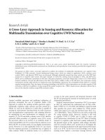
Example 20. Consider the directed graph in Figure 1,which
might be used to represent a MIMO communication scheme.
The adjacency matrix for the directed graph is
A
=
⎡
⎢
⎢
⎢
⎢
⎢
⎢
⎣
0101
0011
0101
1001
⎤
⎥
⎥
⎥
⎥
⎥
⎥
⎦
, (87)
1
2
3

4
Figure 1: A directed graph.
which is a hub matrix with the right-most column cor-
responding to node 4 as the hub column. The associated
arrowhead matrix Q
= A
T
A is
Q
=
⎡
⎢
⎢
⎢
⎢
⎢
⎢
⎣
1001
0202
0011
1214
⎤
⎥
⎥
⎥
⎥
⎥
⎥
⎦

. (88)
The eigenvalues of Q are 0,1,1.4384, 5.5616. Corollary 3
implies 1 being the eigenvalue of Q.ByCorollary 4, the
following matrix

Q =
⎡
⎢
⎢
⎢
⎣
10
√
2
022
√
22 4
⎤
⎥
⎥
⎥
⎦
(89)
should have eigenvalues of λ
1
(

Q) = 0, λ
2
(


Q) = 1.4384,
λ
3
(

Q) = 5.5616. The C bounds, SS bounds, and WS bounds
for the eigenvalues of the matrix

Q are listed in Ta ble 1.For
λ
1
(

Q), the lower SS bound is best; next is the lower C bound
followed by the lower WS bound; the upper SS bound is best;
next is the upper WS bound followed by the upper C bound.
For λ
2
(

Q), SS bounds and C bounds are the same as the C
bounds. For λ
3
(

Q), the lower SS bound is best; the lower C
bound and WS bound are the same; the upper SS bound is
best; next is the upper WS bound followed by the upper C
bound. In conclusion, the SS bounds are best.

The bounds of the eigengap of Q provided by (69)are
2 < EG
1
(
Q
)
< 6
(90)
while the bounds provided by (70)are
2.6861 < EG
1
(
Q
)
< 5.6458.
(91)
Therefore, the bounds by (70) are tighter than those by (69).
This numerically justifies Proposition 19.
Example 21. We consider an arrowhead matrix Q as follows:
Q
=
⎡
⎢
⎢
⎢
⎣
10
√
2
062

√
22 7
⎤
⎥
⎥
⎥
⎦
. (92)
EURASIP Journal on Advances in Signal Processing 11
Table 1: C bounds, SS bounds, and WS bounds for Example 20.
Eigenvalues
C bounds SS bounds WS bounds
Lower Upper Lower Upper Lower Upper
λ
1
(

Q) = 0 −0.4142 1 −0.3723 0.3542 −10.6667
λ
2
(

Q) = 1.4384 1 2 1 2
λ
3
(

Q) = 5.5616 4 7.4142 5.3723 5.6458 4 5.6667
Table 2: C bounds, SS bounds, and WS bounds for Example 21.
Eigenvalues

C bounds SS bounds WS bounds
Lower Upper Lower Upper Lower Upper
λ
1
(Q) = 0.6435 −0.4142 1 0.1270 1 0 2.3333
λ
2
(Q) = 4.6304 1 6 4 6
λ
3
(Q) = 8.7261 6 10.4142 7.8730 9 7 9.3333
Table 3: C bounds, SS bounds, and WS bounds for Example 22.
Eigenvalues
C bounds SS bounds WS bounds
Lower Upper Lower Upper Lower Upper
λ
1
(Q) = 0.6192 0.5000 1 0.2753 0.8820 0.2137 0.9402
λ
2
(Q) = 1.3183 1 2 1 2
λ
3
(Q) = 3.0624 2 3.5000 2.7247 3.1180 2.3931 3.1196
The eigenvalues of Q and the corresponding C bounds,
SS bounds, and WS bounds for the eigenvalues of Q are listed
in Ta ble 2.Forλ
1
(Q), the lower SS bound is the best; next is
the lower WS bound followed by the lower C bound; the SS

upper bound and the C upper bound are the same and are
better than the upper WS bound. For λ
2
(Q), the lower SS
bound is better than the lower C bound; the upper SS bound
is the same as the upper C bound. For λ
3
(Q), the lower SS
bound is the best; next is the lower WS bound followed by
the lower C bound; the upper SS bound is the best; next is
the upper WS bound followed by the upper C bound.
Example 22. We consider an arrowhead matrix Q as follows:
Q
=
⎡
⎢
⎢
⎢
⎢
⎢
⎢
⎣
10
1
2
021
1
2
12
⎤

⎥
⎥
⎥
⎥
⎥
⎥
⎦
. (93)
The eigenvalues of Q and the corresponding C bounds,
SS bounds, and WS bounds for the eigenvalues of Q are listed
in Ta ble 3.Forλ
1
(Q), the lower C bound is best; next is the
lower SS bound followed by the lower WS bound; the upper
SS bound is the best; next is the upper WS bound followed by
the upper C bound. For λ
2
(Q), the SS bounds are the same
as the C bounds. For λ
3
(Q), the upper SS bound is the best;
next is the upper WS bound followed by the upper C bound;
the SS lower bound is the best; next is the lower WS bound
followed by the lower C bound.
6. Conclusions
Motivated by the need to more accurately estimate eigengaps
of the system matrices associated with hub matrices, this
paper provides an efficient way to estimate the lower and
upper bounds of arrowhead matrices. Improved lower and
upper bounds for the eigengaps of the system matrices are

developed. We applied these results to a wireless computation
application, and subsequently we presented several numeri-
cal examples. In the future, we will plan to extend our results
to hub dominant matrices, which will allow hub matrices
with correlated nonhub columns.
Acknowledgments
The research was supported by the Air Force Visiting
Summer Faculty Program and by the US National Science
Foundation under Grant DMS-0712827.
References
[1] M. Bixon and J. Jortner, “Intramolecular radiationless transi-
tions,” The Journal of Chem ical Physics, vol. 48, no. 2, pp. 715–
726, 1968.
[2] J. W. Gadzuk, “Localized vibrational modes in Fermi liquids.
General theory,” Physical Review B, vol. 24, no. 4, pp. 1651–
1663, 1981.
[3] D. P. O’Leary and G. W. Stewart, “Computing the eigenvalues
and eigenvectors of symmetric arrowhead matrices,” Journal of
Computational Physics, vol. 90, no. 2, pp. 497–505, 1990.
[4] K. Dickson and T. Selee, “Eigenvectors of arrowhead matrices
via the adjugate,” preprint, 2007.
12 EURASIP Journal on Advances in Signal Processing
[5] D. Boley and G. H. Golub, “A survey of matrix inverse
eigenvalue problems,” Inverse Problems, vol. 3, no. 4, pp. 595–
622, 1987.
[6] B. Parlett and G. Strang, “Matrices with prescribed Ritz
values,” Linear Algebra and Its Applications, vol. 428, no. 7, pp.
1725–1739, 2008.
[7] J. Peng, X Y. Hu, and L. Zhang, “Two inverse eigenvalue
problems for a special kind of matrices,” Linear Algebra and

Its Applications, vol. 416, no. 2-3, pp. 336–347, 2006.
[8] H. Pickmann, J. Ega
˜
na, and R. L. Soto, “Extremal inverse
eigenvalue problem for bordered diagonal matrices,” Linear
Algebra and Its Applications, vol. 427, no. 2-3, pp. 256–271,
2007.
[9]H.T.KungandB.W.Suter,“AHubmatrixtheoryand
applications to wireless communications,” EURASIP Journal
on Advances in Signal Processing, vol. 2007, Article ID 13659, 8
pages, 2007.
[10] J. M. Kleinberg, “Authoritative sources in a hyperlinked
environment,” Journal of the ACM, vol. 46, no. 5, pp. 604–632,
1999.
[11] D. Tse and P. Viswanath, Fundamentals of Wireless Communi-
cation, Cambridge University Press, Cambridge, UK, 2005.
[12]R.A.HornandC.R.Johnson,Matrix Analysis, Cambridge
University Press, Cambridge, UK, 1985.
[13] E. Montano, M. Salas, and R. Soto, “Positive matrices with
prescribed singular values,” Proyecciones,vol.27,no.3,pp.
289–305, 2008.
[14] R. Bhatia, Matrix Analysis, vol. 169 of Graduate Texts in
Mathematics, Springer, New York, NY, USA, 1997.
[15] H. Wolkowicz and G. P. H. Styan, “Bounds for eigenvalues
using traces,” Linear Algebra and Its Applications, vol. 29, pp.
471–506, 1980.