Báo cáo hóa học: " Research Article An MLP Neural Net with L1 and L2 Regularizers for Real Conditions of Deblurring" doc

Hindawi Publishing Corporation
EURASIP Journal on Advances in Signal Processing
Volume 2010, Article ID 394615, 18 pages
doi:10.1155/2010/394615
Research Article
An MLP Neural Net with L1 and L2 Regularizers for
Real Conditions of Deblurring
Miguel A. Santiago,
1
Guillermo Cisneros,
1
and Emiliano Bernu
´
es
2
1
Depart amento de Se
˜
nales, Sistemas y Radiocomunicaciones, Escuela T
´
echica Superior de Ingenieros de Telecomunicaci
´
on,
Universidad Polit
´
ecnica de Madrid, 28040 Madrid, Spain
2
Departamento de Ingenier
´
ıa Electr
´

onica y Comunicaciones, Centro Polit
´
ecnico Superior, Universidad de Zaragoza,
50018 Zaragoza, Spain
Correspondence should be addressed to Miguel A. Santiago,
Received 19 March 2010; Revised 2 July 2010; Accepted 6 September 2010
Academic Editor: Enrico Capobianco
Copyright © 2010 Miguel A. Santiago et al. This is an open access article distributed under the Creative Commons Attribution
License, which permits unrestricted use, distribution, and reproduction i n any medium, provided the original work is properly
cited.
Real conditions of deblurring involve a spatially nonlinear process since the borders are truncated, causing significant artifacts
in the restored results. Typically, it is assumed to have boundary conditions to reduce ringing; in contrast, this paper proposes
a restoration method which simply deals with null borders. We minimize a deterministic regularized function in a Multilayer
Perceptron (MLP) w ith no training and follow a back-propagation algorithm with the L1 and L2 norm-based regularizers. As a
result, the truncated borders are regenerated while adapting the center of the image to the optimum linear solution. We report
experimental results showing the good performance of our approach in a real model without borders. Even if using boundary
conditions, the quality of restoration is comparable to other recent researches.
1. Introduction
Image restoration is a classical topic of digital image
processing, appear ing in many applications such as remote
sensing, medical imaging, astronomy, or digital photography
[1]. This problem aims to invert a degradation process
for recovering the or iginal image, but it is mathematical ly
ill-posed and leads to a highly noise sensitive solution.
Consequently, a large number of techniques have been
developed to deal with this issue, most of them under
the regularization or the Bayesian frameworks (a complete
review can found in [2–4]).
The degraded image in those methods comes from the
acquisition of a scene in a finite domain (field of view)

and exposed to the effects of blurring and additive noise.
The image blur is generally modeled as a convolution of
the unknown true image with a point spread function
(PSF). However, the nonlocal property of the convolution
implies that part of the blurred image near the bound-
ary integrates information of the original scenery outside
the field of view. This information is not available in
the deconvolution process and may cause strong ringing
artifacts on the restored image, that is, the well-known
boundary problem [5]. Various methods to counteract the
boundary effect have been proposed in the literature,
making assumptions about the behavior of the original
image outside the field of view such as Dirichlet, Neuman,
periodic, or other recent conditions in [6–8]. Depending
on the boundary assumptions, the blurring matrix adopts
a structure with particular computational properties. In
fact, the periodic convolution is frequently assumed in the
restoration model as the computations can be efficiently per-
formed with block circulant matrices, compared to the block
Toeplitz matrixes of the zero-Dirichlet conditions (aper iodic
model).
In this paper, we present a restoration method which
also starts with a real blurred image in the field of view, but
with neither any image information nor prior assumption on
the boundary conditions. Furthermore, the objective is not
only to improve the restoration on the whole image, but also
reconstruct the unknown boundaries of the original image
without prior assumption.
2 EURASIP Journal on Advances in Signal Processing
L

2
L
1
Field
of
view
Circulant
Aperiodic
(M
2
− 1)/2
(M
2
− 1)/2
(M
1
− 1)/2
(M
1
− 1)/2
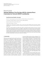
Figure 1: Real observed image which truncates the borders
appeared in the circulant and the aperiodic models.
Neural networks are very well suited to combine both
processes through the same restoration algorithm, in line
with a given adaptation strategy. It could be thought that
neural nets are able to learn about the degradation model,
and so the borders of the image may be regenerated.
For that reason, the algorithm of this paper uses a sim-
ple Multilayer Perceptron (MLP) based on the strateg y
of back-propagation. Others neural-net-based restoration

techniques[9–11] have b een proposed in the literature with
the Hopfield’s model however, they tend to be time-
consuming and large scaled. Besides, a Laplace operator is
normally used as regularization term in the energy function
(
2
regularizer) [9–13], but the success of the TV (total
variation) regularization in deconvolution [14–18], also
referred as 
1
regularizer in this paper, has motivated its
incorporation into our MLP.
A first step of our neural net was given in a previous
work [19] using the standard 
2
norm. Here, we propose
a newer analysis of the problem on the basis of matrix
algebra, using the TV regularizer of [17] and showing a wide
range of results. A future research may be addressed to other
more effective regularizations terms such as the nonlocal
regularization in [20, 21].
Let us note that our paper builds somehow on the
same algorithmic base presented for the authors in this
Journal about the desensitization problem [22]. In fact,
our MLP simulates at every iteration an approach to both
the degradation (backward) and the restoration (forward)
processes, thus extending the same iterative concept but
applied to a nonlinear problem. Let us remark that we use
here the words “backward” and “forward” in the context of
our neural net, which is the opposite sense in a standard

image restoration.
This paper is structured as follows. In the next section,
we provide a detailed formulation of the problem, estab-
lishing naming conventions and the energy functions to be
minimized. In Section 3, we present the architecture of the
neural net under analysis. Section 4 describes the adjust ment
of its synaptic weights in ever y l ayer for both 
2
and 
1
regularizers and outlines the reconstruction of borders. We
present some experimental results in Section 5 and, finally,
concluding remarks are given in Section 6.
2. Problem Formulation
Let h(i, j) be any generic two-dimensional degradation filter
mask (PSF, usually invariant low-pass filter) and x(i, j) the
unknown original image, which can be lexicographically
represented by the vectors h and x
h
=
[
h
1
, h
2
, , h
M
]
T
,

x
=
[
x
1
, x
2
, , x
L
]
T
,
(1)
where M
= [M
1
× M
2
] ⊂ R
2
and L = [L
1
× L
2
] ⊂ R
2
are the
respective supports of the PSF and the original image.
A classical formulation of the degradation model (blur
andnoise)inanimagerestorationproblemisgivenby

y
= Hx + n,(2)
where H is the blurring matrix corresponding to the filter
mask h of (1), y is the observed image (blurred and noisy
image), and n is a sample of a zero mean white Gaussian
additive noise of variance σ
2
.
The matrix H can be generally expressed as
H
= T + B,(3)
where T has a Toeplitz st ructure and B,whichisdefined
by the boundary conditions, is often structured, sparse, and
low rank. Boundary conditions (BCs) make assumptions
about how the observed image behaves outside the field
of view (FOV), and they are often chosen for algebraic
and computational convenience. The following cases a re
commonly referenced in literature.
Zero BCs [23], aka Dirichlet, impose a black boundary so
that the matrix B is all zeros, and, therefore, H has a Toeplitz
structure (BTTB). This implies an artificial discontinuity at
the borders which can lead to serious ringing effects.
Periodic BCs [23], aka Neumann, assume that the scene
can be represented as a mosaic of a single infinite dimen-
sional image, repeated periodically in all directions. The
resulting matrix H is BCCB which can be diagonalized by the
unitary discrete Fourier transform and leads to a restoration
problem implemented by FFTs. Although computationally
convenient, it cannot actually represent a physical observed
image and still produces ringing artifacts.

Reflective BCs [24] reflect the image like a mirror with
respect to the boundaries. In this case, the matrix H has a
Toeplitz-plus-Hankel structure w hich can be diagonalized by
the orthonormal discrete cosine transformation if the PSF is
symmetric. As these conditions maintain the continuity of
the graylevel of the image, the ringing effects are reduced in
the restoration process.
EURASIP Journal on Advances in Signal Processing 3
Antireflective BCs [7], similarly reflect the image with
respect to the boundaries but using a central symmetry
instead of the axial sy mmetry of the reflective BCs. The
continuity of the image and the normal derivative are
both preserved at the boundary leading to an important
reduction of ringing. The structure of H is Toeplitz-plus-
Hankel and a structured rank 2 matrix, which can be also
efficiently implemented if the PSF satisfies a strong symmetry
condition.
As a result of these BCs, the matrix product Hx in (2)
yields a vector y of length

L,whereH is

L × L in size
and the value of

L depends on the convolution operator.
We will mainly analyze the cases of the aperiodic model
(linear convolution plus zero BCs) and the circulant model
(circular convolution plus periodic BCs) whose parameters
are summarized in Table 1 . Regarding the reflective and

antireflective BCs, they can be managed as an extension of
the aperiodic problem, by setting the appropriate boundaries
to the original image x.
Then,wecomeupwithadegradedimagey of support

L ⊂ R
2
with borders derived from the boundary conditions,
however, they are not actually present in a real observation.
Figure 1 illustrates the borders resulted in the aperiodic and
circulant models, and defines the region FOV as
FOV
=
[
(
L
1
− M
1
+1
)
×
(
L
2
− M
2
+1
)
]

⊂

L. (4)
Arealobservedimagey
real
is, therefore, a truncation of
the degradation model up to the size of the FOV support.
In our algorithm, we define an image y
tru
which represents
this observed image y
real
by means of a truncation on the
aperiodic model
y
tru
= trunc{H
a
x + n},(5)
where H
a
is the blurring matrix for the aperiodic model
and the operator trunc
{·} is responsible for removing (zero-
fixing) the borders appeared due to the boundary conditions,
that is to say
y
tru

i, j


=
trunc

H
a
x + n|
(i, j)

=
⎧
⎨
⎩
y
real
= H
a
x + n|
(i, j)
∀

i, j

∈ FOV
0 otherwise
⎫
⎬
⎭
.
(6)

Dealing with a truncated image like (6) in a restoration
problem is an evident source of ringing for the discontinuity
at the boundaries. For that reason, this paper aims to provide
an image restoration approach to avoid those undesirable
ringing artifacts when y
tru
is the observed image. Further-
more, it is also intended to regenerate the truncated borders
while adapting the center of the image to the optimum linear
solution.
Even if the boundary conditions are maintained in the
restoration process, our method is able to reduce the ringing
artifacts derived from each boundary discontinuity.
Restoring an image x is usually an ill-posed or ill-
conditioned problem since either the blurring operator
H does not admit inverse or is nearly singular. Hence,
a regularization method should be used in the inversion
process for controlling the high sensitivity to the noise.
Prominent examples have been presented in the literature by
means of the classical Tikhonov regularization
x = arg min
x

1
2


y − Hx



2
2
+
λ
2
Dx
2
2

,(7)
where
z
2
2
=

i
z
2
i
denotes the 
2
norm, x is the restored
image and D is the regularization operator, built on the
basis of a high pass filter mask d of support N
= [N
1
×
N
2

] ⊂ R
2
and using the same boundary conditions described
previously. The first term in (7) is the 
2
residual norm
appearing in the least-squares approach and ensures fidelity
to data. The second term is the so-called “regularizer”or
“side constrain” and captures prior knowledge about the
expected behavior of x through an additional 
2
penalty
term involving just the image. The hyperpara meter (or
regularization parameter) λ is a critical value which measures
the tradeoff between a good fit and a regular ized solution.
Alternatively, the total variation (TV) regularization,
proposed by Rudin et al. [25], has become very popular in
recent research as result of preserving the edges of objects
in the restoration. A discrete version of the TV deblurring
problem is given by
x = arg min
x

1
2


y − Hx



2
2
+ λ∇x
1

,(8)
where
z
1
denotes the 
1
norm (i.e., the sum of the absolute
value of the elements) and
∇ stands for the discrete gradient
operator. The
∇ operator is defined by the matrices D
ξ
and
D
μ
as
∇x =



D
ξ
x




+ |D
μ
x| (9)
built on the basis of the respective masks d
ξ
and d
μ
of support
N
= [N
1
× N
2
] ⊂ R
2
, which turn out the horizontal and
vertical first order differences of the image. Compared to the
expression (7), the TV regular ization provides a 
1
penalty
term which can be thought as a measure of signal variability.
Once again, λ is the critical regularization parameter to
control the weight we assign to the regularizer, relatively to
the data misfit term.
In the remainder of the paper, we will refer indistinctly to
the 
2
regularizer as the Tikhonov model, and, likewise, the


1
regularizer may be mentioned as the TV model.
Significant amount of work has been addressed to solve
any of the above regularizations and mainly the TV deblur-
ring in recent times. Nonetheless, most of the approaches
adopted periodic boundary conditions to cope with the
problem on optimal computation b asis. We now intend
to study 
1
and 
2
regularizers over a suitable restoration
approach which manage not only the typical boundary
4 EURASIP Journal on Advances in Signal Processing
Table 1: Sizes of the variables involved in the degradation process for the circulant, aperiodic, and real models.
Models
size
{x} size{h} size{H} size{y}
L × 1 M × 1

L × L

L × 1
Circulant

L = L,
Aperiodic L
= [L
1
× L

2
] M = [M
1
× M
2
]

L = [(L
1
+ M
1
− 1) × (L
2
+ M
2
− 1)]
Truncated
Truncated image y is defined in the support
FOV
=
⎡
⎢
⎣
(L
1
− M
1
+1)×
(L
2

− M
2
+1)
⎤
⎥
⎦
and the rest are
zerosuptothesamesize

L of the aperiodic
model.
Table 2: Size of the variables involved in the restoration process using 
2
and 
1
regularizers,and particularised to the circulant, aperiodic,
and real degradation models. The support of the regularisation filters for 
2
and 
1
are equally set to N = [N
1
× N
2
].
Regularizer 
2

1
size{x} size{d} size{D} size{Dx} size{d

ξ
}, size{d
μ
} size{D
ξ
}, size{D
μ
} size{D
ξ
x}, size{D
μ
x}
L × 1 N × 1 U × L U × 1 N × 1 U × L U × 1
Models
Circulant
U
= L U = L
Aperiodic
U
= [(L
1
+ N
1
− 1) × (L
2
+ N
2
− 1)] U = [(L
1
+ N

1
− 1) × (L
2
+ N
2
− 1)]
Truncated [N
1
× N
2
]
Truncated image Dx is defined in the
support [(L
1
− N
1
+1)× (L
2
− N
2
+1)]
and the rest are zeros up to the same
size U of the aperiodic model.
N
= [N
1
× N
2
]
Truncated images D

ξ
x and D
μ
x are defined
in the support [(L
1
− N
1
+1)× (L
2
− N
2
+1)]
and the rest are zeros up to the same size U
of the aperiodic model.
conditions, but also the real truncated image as in (5).
Consequently, (7)and(8) can redefined as
x |
2
= arg min
x

1
2


y − trunc{H
a
x}



2
2
+
λ
2
trunc{D
a
x}
2
2

,
(10)
x |
1
= arg min
x

1
2


y − trunc{H
a
x}


2
2

+λ



trunc




D
ξ
a
x



+



D
μ
a
x








1

,
(11)
where the subscript a denotes the aperiodic formulation of
the matrix operator. By removing the operator trunc
{·} from
(10)and(11), and changing it into the specific subscripted
operator can be deduced the models for every boundary
condition (similar comment can be applied to the remainder
of the paper). Table 2 summarizes the dimensions involved
in both regularizations taking into account the information
provided in Ta ble 1 and the definition of the operator
trunc
{·} in (6).
To go through this problem, we know that neural
networks are especially wellsuited as their ability to nonlinear
mapping and self-adaptiveness. In fact, the Hopfield network
has been used in the literature to solve (7), and recent
works are providing neural network solutions to the TV
regularization (8)asin[14, 15]. In this paper, we l ook for
a simple solution to solve both regularizations based on an
MLP (Multiplayer Perceptron) with backpropagation.
3. Definition of the MLP Approach
Let us build our neural net according to the MLP architecture
illustrated in Figure 2. The input layer of the net consists of

L neurons with inputs y
1

, y
2
, , y

L
being, respectively, the

L pixels of the degraded image y.Atanygenericiteration
m, the output layer is defined by L neurons whose outputs
x
1
(m), x
2
(m), , x
L
(m) are, respectively, the L pixels of an
approach
x(m) to the restored image. After m
total
iterations,
the neural net outcomes the actual restored image
x =

x(m
total
). On the other hand, the hidden layer consists of
two neurons, this being enough to achieve good restoration
results while keeping low complexity of the network. In any
case, the next analysis will be generalized for any number of
hidden laye rs and any number of neurons per layer.

Whatever the degradation model used in y, the neural
net works by simulating at every iteration both an approach
to the degradation process (backward) and to the restoration
solution (forward), while refining the results progressively at
every iteration of the net. However, the input to the net at
any iteration is always the degraded image, as no net training
is required. L et us recall that w e manage “backward” and
“forward” concepts in the opposite sense to a standard image
restoration because of the architecture of the net.
During the back-propagation process, the network must
minimize iteratively a regularized error func tion which we
will precisely set to (10)and(11) in the following sections.
Since the trunc
{·} operator is involved in those expressions,
the truncation of the borders is also simulated at every
EURASIP Journal on Advances in Signal Processing 5
y
2
˜
L inputs
y
1
y
˜
L
L outputs
Forward
Backward
y
^x

L
(m)
^x
1
(m)
^x
2
(m)
^x =
^
x(m
total
)
Figure 2:MLPschemeadoptedforimagerestoration.
R inputs
1
R
× 1
S
× R
S
× 1
S × 1
S
× 1
ϕ
S neurons
W
b
v

z
p
Figure 3: Model of a layer in the MLP
iteration a s well as its regeneration, with no a priori knowl-
edge, assumption, or estimation concerning those unknown
borders. Consequently, a restored image is obtained in real
conditions on the basis of a global energy minimization
strategy, with regenerated borders while adapting the centre
of the image to the optimum solution and thus making the
ringing artifact negligible.
Following a similar naming convention to that adopted
in Section 2, let us define any generic layer of the net
composed by R inputs and S neurons (outputs) as illustrated
in Figure 3.
Where p is the R
× 1 input vector, W represents
the synaptic weight matrix, S
× R in size, and z is the
S
× 1 output vector of the layer. The bias vector b is
ignored in our particular implementation. In order to have
adifferentiable transfer function, a log-sigmoid expression is
chosen for ϕ
{·}
ϕ{v}=
1
1+e
−v
, (12)
which is defined in the domain 0 ≤ ϕ{·} ≤ 1.

Then, a layer in the MLP is characterized for
z
= ϕ{v},
v
= Wp + b = Wp,
(13)
as b
= 0 (vector of zeros). Furthermore, two layers are
connected each other verifying that
z
i
= p
i+1
, S
i
= R
i+1
, (14)
Table 3: Summary of dimensions for the output layer.
Regularizer
Output layer

2

1
size{p(m)}
p(m) = z
i−1
(m) ⇒ size{p(m)} = S
i−1

× 1
size
{W(m)}
L × S
i−1
size{v(m)}
L × 1
size
{z(m)}
z(m) = x(m) ⇒ size{z(m)} = L × 1
size
{e(m)}

L × 1
size
{r(m)} U × 1
size
{D}=2U × L ⇒
size{r(m)}=2U × 1and
size
{Ω}=2U × 2U
size
{δ(m)}
L × 1
where i and i + 1 are superscripts to denote two consecutive
layers of the net. Although this superscripting of layers
should b e appended to all variables, for notational simplicity
we will remove it from all formulae of the paper when
deduced by the context.
4. Adjustment of the Neural Net

In this section, our purpose is to show the procedure of
adjusting the interconnection weights as the MLP iterates.
A variant of the well-known algorithm of back-propagation
is applied by solving the optimization problems in (10)and
(11).
Let ΔW
i
(m + 1) be the correction applied to the weight
matrix W
i
of the layer i at the (m +1)
th
iteration. Then,
ΔW
i
(
m +1
)
=−η
∂E
(
m
)
∂W
i
(
m
)
, (15)
where E(m) stands for the restoration error after m iterations

at the output of the net and the constant η indicates the
learning speed. Let us compute now the so-called gradient
matrix (∂E(m))/(∂W
i
(m)) for 
2
and 
1
regularizers in any of
the layers of the MLP.
4.1. Output Layer
4.1.1. 
2
Regularizer. Defining the vectors e(m)andr(m)for
the respective error and regular ization terms at the output
layer after m iterations
e
(
m
)
= y − trunc

H
a
x
(
m
)

,

r
(
m
)
= trunc

D
a
x
(
m
)

,
(16)
we can rewrite the restoration error in a 
2
regularizer
problemfrom(10)as
E
(
m
)
=
1
2
e
(
m
)


2
2
+
1
2
λ
r
(
m
)

2
2
. (17)
Using the matrix chain rule when having a composition
on a vector [26], the gradient matrix leads to
∂E
(
m
)
∂W
(
m
)
=
∂E
(
m
)

∂v
(
m
)
·
∂v
(
m
)
∂W
(
m
)
= δ
(
m
)
·
∂v
(
m
)
∂W
(
m
)
. (18)
6 EURASIP Journal on Advances in Signal Processing
Layer 1
Layer 2

L
2
L
2
− M
2
+1
L
1
− M
1
+1
˜
L
× 1
S
1
×
˜
L
S
1
× 1 S
1
× 1
S
1
× 1
L
× S

1
L × 1
L
× 1
L
1
˜
L inputs S
1
neurons S
1
inputs L neurons
ΔW
1
=−ηδ
1
y
T
p
1
= y
W
1
v
1
ϕϕ
z
1
ΔW
2

=−ηδ
2
(z
1
)
T
p
2
v
2
W
2
z
2
=
^
x
Figure 4: MLP algorithm specifically used in the experiments for J = 2.
(a) (b) (c)
Figure 5: Lena image 256 × 256 in size degraded by uniform blur 7 × 7 and BSNR = 20 dB: (a) TRU, (b) APE, and (c) CIR.
where δ(m) = (∂E(m))/(∂v(m)) is the so-called local
gradient vector which again can expanded by the chain rule
for vectors [27]
δ
(
m
)
=
∂z
(

m
)
∂v
(
m
)
·
∂E
(
m
)
∂z
(
m
)
. (19)
Since z and v are elementwise related by the transfer
function ϕ
{·} and thus (∂z
i
(m))/(∂v
j
(m)) = 0foranyi
/
= j,
then
∂z
(
m
)

∂v
(
m
)
= diag

ϕ

{v
(
m
)
}

, (20)
representing a diagonal matrix whose eigenvalues are
computed by the function
ϕ

{v}=
e
−v
(
1+e
−v
)
2
. (21)
We recall that z(m)isactually
x(m) in the output layer

(see Figure 2). Hence, we can compute the second multiplier
of (19) by applying matrix calculus basis over the expressions
(16), and (17). A detailed computation can be found in the
appendix and leads to
∂E
(
m
)
∂z
(
m
)
=
∂E
(
m
)
∂x
(
m
)
=−H
T
a
e
(
m
)
+ λD
T

a
r
(
m
)
. (22)
According to the Tables 1 and 2,(∂E(m))/(∂z(m))
represents a vector of size L
× 1. When combining with the
diagonal matrix of (20), we can write
δ
(
m
)
= ϕ


v
(
m
)

◦

−
H
T
a
e
(

m
)
+ λD
T
a
r
(
m
)

. (23)
where
◦ denotes the Hadamard (elementwise) product.
To complete the analysis of the gradient matrix, we have
to compute the term (∂v(m))/(∂W(m)). Based on the layer
definition in the MLP (13), we obtain
∂v
(
m
)
∂W
(
m
)
=
∂W
(
m
)
p

(
m
)
∂W
(
m
)
= p
T
(
m
)
, (24)
which in turns corresponds to the output of the previous
connected hidden layer, that is to say
∂v
(
m
)
∂W
(
m
)
=

z
i−1
(m)

T

. (25)
EURASIP Journal on Advances in Signal Processing 7
10
10
12
12
14
14
16
16
18
18
20
20
22
22
24
24
26
26
28
28
30
30
6
7
8
9
10
11

12
13
14
6
7
8
9
10
11
12
13
14
BSNR (dB)
TRU
APE
CIR
σ
e
with L2 regularizer
σ with L1 regularizer
(a)
10
10
12
12
14
14
16
16
18

18
20
20
22
22
24
24
26
26
28
28
30
30
6
7
8
9
10
11
12
13
BSNR (dB)
TRU
APE
CIR
4
5
6
7
8

9
10
11
12
13
4
5
σ
e
with L2 regularizer
σ with L1 regularizer
(b)
Figure 6: Restoration error σ
e
for 
2
and 
1
regularizers using TRU, APE, and CIR degradation models: (a) filter h
1
(b) filter h
2
.
0.005
0.01
0.015
0.02
0.025
0.5
1

1.5
8.5
8.6
8.7
8.8
8.9
9
λ
η
σ
e
Figure 7: Sensitivity of σ
e
to η and λ.
Putting together all the results into the incremental
weight matrix ΔW(m +1),wehave
ΔW
(
m +1
)
=−ηδ
(
m
)

z
i−1
(m)

T

=−η

ϕ


v
(
m
)

◦

−
H
T
a
e
(
m
)
+ λD
T
a
r
(
m
)


×


z
i−1
(m)

T
.
(26)
4.1.2. 
1
Regularizer. In the light of the above regularizer, let
us also define analogous error and regularization terms with
respect to (8)
e
(
m
)
= y − trunc

H
a
x
(
m
)

,
(27)
r
(

m
)
= trunc




D
ξ
a
x
(
m
)



+



D
μ
a
x
(
m
)





. (28)
With these definitions, E(m)canbewritteninacompact
notation as
E
(
m
)
=
1
2
e
(
m
)

2
2
+ λr
(
m
)

1
. (29)
If we aimed to compute the gradient matrix ∂E(m)/
∂W
i
(m)with(29), we would find out a challenging nonlinear

optimization problem that is caused by the nondifferentiabil-
ity of the 
1
norm. One approach to ov ercome this challenge
comes from
r
(
m
)

1
≈ TV

x
(
m
)

=

k


D
ξ
a
x(m)

2
k

+

D
μ
a
x(m)

2
k
+ ε,
(30)
where TV stands for the well-known total variation reg-
ularizer and ε>0 is a constant to avoid singularities
when minimizing. Both products D
ξ
a
x(m), and D
μ
a
x(m)are
subscripted by k meaning the kth element of the respective
U
× 1 sized vector (see Ta bl e 2). It should be mentioned
that 
1
norm and TV regularizations are quite often used
as the same in the literature. But the distinction between
these two regularizers should b e kept in mind since, at least
in deconvolution problems, TV leads to significant better
results as illustrated in [16].

Bioucas-Dias et al. [16, 17] proposed an interesting
formulation of the total variation problem by applying
majorization-minimization algorithms (MM). It leads to a
quadratic bound function for TV regularizer, which thus
results in solving a linear system of equations. Likewise, we
adopt that quadratic majorizer in our particular implemen-
tation as
TV

x
(
m
)

≤ Q
TV

x
(
m
)

= x
T
(
m
)
D
T
a

Ω
(
m
)
r
(
m
)
+ K, (31)
8 EURASIP Journal on Advances in Signal Processing
where K is an irrelevant constant, the involved matrixes are
defined as
D
a
=


D
ξ
a

T

D
μ
a

T

T

,
Ω
(
m
)
=
⎡
⎣
Λ
(
m
)
0
0 Λ
(
m
)
⎤
⎦
,
(32)
with
Λ
(
m
)
= diag
⎛
⎜
⎜

⎝
1
2


D
ξ
a
x
(
m
)

2
+

D
μ
a
x
(
m
)

2
+ ε
⎞
⎟
⎟
⎠

, (33)
and the regularization term r(m)of(28) is reformulated
r
(
m
)
= trunc

D
a
x
(
m
)

, (34)
such that the operator trunc
{·} works by applying it
individually for D
ξ
a
and D
μ
a
(see Table 2) and merging later
as indicated in the definition of (32).
Finally, we can rewrite the restoration error E(m)as
E
(
m

)
=
1
2
e
(
m
)

2
2
+ λQ
TV

x
(
m
)

. (35)
Thesamestepsasin
2
regularizer can be followed now
to compute the gradient matrix. When we come to resolve
the differentiation (∂E(m))/(∂z(m)), we take advantage of
the quadratic properties of the expression (31) and the
derivation of (22)soastoobtain
∂E
(
m

)
∂z
(
m
)
=
∂E
(
m
)
∂x
(
m
)
=−H
T
a
e
(
m
)
+ λD
T
a
Ω
(
m
)
r
(

m
)
. (36)
It can be deduced as an extension of the 
2
solution
when using the first-order differences operator D
a
of (32)
and incorporating the weigh matrix Ω(m). In fact, this
spatially varying matrix is responsible for the smoothness or
sharpness (presence of edges) of the solution depending on
the local differences of the image.
The remaining steps for the analysis of (∂E(m))/(∂W(m))
are identical to the previous section and yield a local gradient
vector as
δ
(
m
)
= ϕ


v
(
m
)

◦


−
H
T
a
e
(
m
)
+ λD
T
a
Ω
(
m
)
r
(
m
)

, (37)
Finally, we come to the following variation of the weight
matrix
ΔW
(
m +1
)
=−ηδ
(
m

)

z
i−1
(
m
)

T
=−η

ϕ


v
(
m
)

◦

−
H
T
a
e
(
m
)
+λD

T
a
Ω
(
m
)
r
(
m
)


×

z
i−1
(
m
)

T
.
(38)
4.2. Any i Hidden Layer. If we set superscripting for the
gradient matrix (18)overanyi hidden layer of the MLP, we
obtain
∂E
(
m
)

∂W
i
(
m
)
=
∂E
(
m
)
∂v
i
(
m
)
·
∂v
i
(
m
)
∂W
i
(
m
)
= δ
i
(
m

)
·
∂v
i
(
m
)
∂W
i
(
m
)
, (39)
and taking what was already demonstrated in (25), then
∂E
(
m
)
∂W
i
(
m
)
= δ
i
(
m
)

z

i−1
(
m
)

T
. (40)
Let us expand the local gradient δ
i
(m) by means of the
chainruleforvectorsasfollows:
δ
i
(
m
)
=
∂E
(
m
)
∂v
i
(
m
)
=
∂z
i
(

m
)
∂v
i
(
m
)
·
∂v
i+1
(
m
)
∂z
i
(
m
)
·
∂E
(
m
)
∂v
i+1
(
m
)
, (41)
where (∂z

i
(m))/(∂v
i
(m)) is the same diagonal matrix
(20), whose eigenvalues are represented by ϕ

{v
i
(m)},and
(∂E(m))/(∂v
i+1
(m)) denotes the local gradient δ
i+1
(m)of
the following connected layer. With respect to the term
(∂v
i+1
(m))/(∂z
i
(m)), it can be immediately derived from the
MLP definition of (13) that
∂v
i+1
(
m
)
∂z
i
(
m

)
=
∂W
i+1
(
m
)
p
i+1
(
m
)
∂z
i
(
m
)
=
∂W
i+1
(
m
)
z
i
(
m
)
∂z
i

(
m
)
=

W
i+1
(m)

T
.
(42)
Consequently, we come to
δ
i
(
m
)
= diag

ϕ


v
i
(
m
)

W

i+1
(
m
)

T
δ
i+1
(
m
)
, (43)
which can be simplified after verifying that (W
i+1
(m))
T
δ
i+1
(m)
stands for a R
i+1
× 1 = S
i
× 1vector
δ
i
(
m
)
= ϕ



v
i
(
m
)

◦


W
i+1
(
m
)

T
δ
i+1
(
m
)

. (44)
We finally provide an equation to compute the incremen-
tal weight matrix ΔW
i
(m +1)foranyi hidden layer
ΔW

i
(
m +1
)
=−ηδ
i
(
m
)

z
i−1
(m)

T
=−η

ϕ


v
i
(
m
)

◦


W

i+1
(m)

T
δ
i+1
(
m
)

,
×

z
i−1
(m)

T
(45)
which is mainly based on the local gradient δ
i+1
(m) of the
following connected layer i +1.
It is worthy to mention that we have not made any
distinction between regularizers. Precisely, the term δ
i+1
(m)
is in charge of propagating which regularizer is used when
processing the output layer.
EURASIP Journal on Advances in Signal Processing 9

(a) (b) (c)
Figure 8: Restoration results from the Lena degraded image by uniform blur 7 × 7, BSNR = 20 dB and TRU model (a). Respectively for 
2
and 
1
, the restored images are shown in (b) and (c). A broken white line highlights the regeneration of borders.
Initialization: p
1
= y forall m and W
i
(0) = 0 1 ≤ i ≤ J
(1) m :
= 0
(2) while StopRule not satisfied do
(3) for i :
= 1toJ do /
∗
Forward
∗
/
(4) v
i
:= W
i
p
i
(5) z
i
:= ϕ{v
i

}
(6) end f or /
∗
x(m):= z
J ∗
/
(7) for i :
= J to 1 do /
∗
Backward
∗
/
(8) if i
= J then /
∗
Output layer
∗
/
(9) if 
= 
2
then
(10) Compute δ
J
(m)from(23)
(11) Compute E(m)from(17)
(12) elseif 
= 
1
then

(13) Compute δ
J
(m)from(37)
(14) Compute E(m)from(35)
(15) end if
(16) else
(17) δ
i
(m):= ϕ

{v
i
(m)}◦((W
i+1
(m))
T
δ
i+1
(m))
(18) end if
(19) ΔW
i
(m +1):=−ηδ
i
(m)(z
i−1
(m))
T
(20) W
i

(m +1):= W
i
(m)+ΔW
i
(m +1)
(21) end for
(22) m :
= m +1
(23) end while /
∗
x := x(m
total
)
∗
/
Algorithm 1: MLP with  regularizer.
4.3. Algorithm. As described in Section 3,ourMLPneural
net works by performing a couple of forward and backward
processes at every iteration m. Firstly, the whole set of
connected layers propagate the degraded image y from the
input to the output layers by means of (13). Afterwards, the
new synaptic weigh matrixes W
i
(m+1) are recalculated from
right to left according to the expressions of ΔW
i
(m +1)for
every layer.
The previous pseudocode summarizes our proposed
algorithm for 

1
and 
2
regularizers in a MLP of J layers.
There, StopRule denotes a condition such that either the
number of iterations is more than a maximum or the error
E(m) converges, and thus, the error change ΔE(m)isless
than a threshold, or, even, this error E(m) starts to increase. If
one of these conditions comes true, the algorithm concludes
and the final outgoing image is just the restored image
x :=

x(m
total
).
4.4. Regeneration of Borders. If we particularize the algorithm
for two layers J
= 2, we come to a MLP scheme such as
illustrated in Figure 4. It is worthy to emphasize how the
borders are regenerated at any iteration of the net, from a
real image of support FOV(4) to the restored image of size
L
= [L
1
× L
2
] (recall that the remainder of pixels in y was
zerofixed). Additionally, we will observe in Section 5 how
the boundary artifacts are removed from the restored image
based on the energy minimization E(m), but they are critical,

however, for other methods of the literature.
4.5. Adjustment of λ and η. In the image restoration field, it is
wellknown how important the parameter λ becomes. In fact,
too small values of λ yield overly oscillatory estimates owing
to either noise or discontinuities, too large v alues of λ yield
over smoothed estimates.
For that reason, the literature has given significant
attention to it with popular approaches such as the unbiased
predictive risk estimator (UPRE), the generalized cross
validation (GCV), or the L-curve method; see [28]foran
overview and references. Most of them were particularized
for a Tikhonov regularizer, but lately researches aim to
provide solutions for TV regularization. Specifically, the
Bayesian framework leads to successful approaches in this
field.
Since we do not have yet a particular algorithm to adjust
λ in the MLP, then we will take solutions coming from the
Bayesian state-of-art. However, let us recall that most of
them are developed when assuming a circulant model for the
observed image and, thus, not optimized for the aperiodic
10 EURASIP Journal on Advances in Signal Processing
(a) (b) (c)
Figure 9: Restoration results from the Cameraman degraded image by Gaussian blur 7× 7, BSNR = 20 dB and TRU model (a). Respectively
for 
2
and 
1
, the restored images are shown in (b) σ
e
= 16.08 and (c) σ

e
= 15.74.
Figure 10: Artifacts appeared when removing the boundary
conditions, cropping the center, in a MM1 algorithm. With zeros
outside, the restoration is completely corrupted.
or truncated models of this paper. We will summarize the
equations which have better adapted to our neural net in the
following subsections.
It is important to note that λ must be computed for every
iteration m of the MLP. Consequently, as the solution
x(m)
approaches to the final restored image, the regularization
parameter λ(m) also tends to its optimum value. So, in order
to obtain better results, a second computation of the whole
neural net will be executed fixing the previous λ(m
total
).
Regarding the learning speed η, we will empirically
observe in Section 5 that shows lower sensitivity compared
to λ. In fact, its main purpose is to speed up or slow down
the convergence of the algorithm. Then, for the sake of
simplicity, we assume η
= 1orη = 2 depending on the size
of the image.
4.5.1. 
2
Regularizer. Molina et al. [29]dealwiththe
estimation of the hyperparameters α and β (λ
= α/β)
under a Bayesian paradigm for a 

2
regularization as in
(7). So, assuming a simultaneous autoregressive (SAR) prior
distribution for the original image, we can express their
results in terms of our variables as
1
α
(
m
)
=
1

L
r(m)
2
2
+
1
L
trace

Q
−1

α, β

D
T
a

D
a

,
1
β
(
m
)
=
1

L
e(m)
2
2
+
1
L
trace

Q
−1

α, β

H
T
a
H

a

,
(46)
where Q(α, β)
= α(m − 1)D
T
a
D
a
+ β(m − 1)H
T
a
H
a
and
no a priori information about the parameters is included.
Consequently, the regularization parameter is obtained for
every iteration as λ(m)
= α(m)/β(m).
Nevertheless, computing the inverse of the matrix
Q(α, β) for relative medium sized images turns out a heavy
task in terms of computational cost. For that reason, we
approximate the second term of (46) considering block
circulant matrices also for the aperiodic and truncated
models. It means that we can efficiently process the matrix
inversion via a 2D FFT, based on the frequency properties of
the circulant model. In any case, an iterative method could
have been also used to compute Q
−1

(α, β) without relying on
circulant matrices [30].
4.5.2. 
1
Regularizer. In search of another Bayesian fashion
solution for λ, but now applied to the TV regularization
problem, we come across the proposed analysis of Bioucas-
Dias et al. [17]. By using a Gamma prior for λ,itleadsto
λ
(
m
)
=
ρσ
2
TV


x
(
m
)

+ β
,
(47)
ρ
= 2
(
α + θ · L

)
,
(48)
where TV
{x(m)} waspreviouslydefinedin(30)andα,
β are the respective shape and scale parameters of the
Gamma distribution p(λ/α, β)
∝ λ
α−1
exp(−βλ). In any case,
these two parameters have not such an influence on the
computation of λ as α
 θ·L and β  TV{x(m)}. Regarding
EURASIP Journal on Advances in Signal Processing 11
(a) (b)
(c) (d)
Figure 11: Restoration results from the Cameraman degraded image by Gaussian blur 7×7, BSNR = 20dBandCIRmodel(a).Therestored
images are shown for (b) 
1
-MLP: σ
e
= 15.55, (c) MM2: σ
e
= 14.73, and (d) TV1: σ
e
= 15.98.
40 50 60 70 80 90 100 110 120
13.5
14
14.5

15
Iterations
σ
e
Zero
Periodic
Reflective
Anti-reflective
(a)
20
30 40 50 60
70 80 90
100
11.2
11.4
11.6
11.8
12
12.2
12.4
12.6
12.8
13
13.2
Iterations
σ
e
Zero
Periodic
Reflective

Anti-reflective
(b)
Figure 12: Evolution of the restoration error σ
e
in a 
2
-MLP for the boundary conditions: zero, periodic, reflective, and antireflective. Two
different plots are shown using a Barbara degraded image by a 7
× 7 (a) uniform blur and a (b) diagonal motion blur.
12 EURASIP Journal on Advances in Signal Processing
(a) (b)
Figure 13: Restoration results from the B arbara degraded image by a Gaussian blur 7 × 7, BSNR = 20dBandzeroBC.Therestoredimages
are shown for (a) CGLS: σ
e
= 14.06 and (b) 
1
-MLP: σ
e
= 12.56.
(a) (b)
Figure 14: Restoration results from the Barbara degraded image by a diagonal motion blur 7 × 7, BSNR = 20 dB and antireflective BC. The
restored images are show n for (a) CGLS: σ
e
= 12.29 and (b) 
2
-MLP: σ
e
= 11.80.
the constant 0 <θ<1, it is adjusted to get better results of
the algorithm and we will provide a heuristic value on a trial

and error basis.
5. Experimental Results
A number of exper iments have been performed with the
proposed MLP using several standard images and PSFs,
some of which are presented here. The aim is to test the
restoration results and the border regeneration properties
when considering a real situation of deblurring (truncated
model). Moreover, we will evaluate the results when assumed
different boundary conditions in the obser ved image. Let
us refer to the truncated, aperiodic and circulant models as
TRU, APE and CIR henceforth.
Figure 5 depicts the original Lena image 256
× 256 in size
of Experiment 1 which is blurred according to those three
degradations models. We can observe the zero truncation of
borders i n TRU, the expansion of the aperiodic convolution
of APE and the circular assumption of boundaries in CIR
(review Figure 1). We note here the larger size

L of APE
and TRU against to the original size L of CIR. Nonetheless,
it should be remarked that the TRU image of Figure 5(a)
corresponds to the model y
tru
of (6) and the real observed
image y
real
is actually the region defined in FOV, that is,
250
× 250. Zeros outside the FOV are merely related to the

MLP, but not to the real blurred data.
Let us recall that our algorithm is divided into two
different implementations depending on the regularization
term of E(m), either Tikhonov or TV. Then, we particularize
the filter mask d of the operator D by means of the Laplace
operator with the 
2
regularizer (7)
1
6
⎡
⎢
⎢
⎢
⎣
141
4
−20 4
141
⎤
⎥
⎥
⎥
⎦
, (49)
EURASIP Journal on Advances in Signal Processing 13
Table 4: Numerical values of σ
e
for 
2

and 
1
regularizers compared with those obtained when λ is estimated according to the algorithms of
Section 4.5. The results are divided into the degradation model TRU, APE and CIR, as well as the filters h
1
and h
2
.
h
1
Regularizer 
2
-norm 
1
-norm
σ
e
λ optimum λ estimated λ optimum λ estimated
BSNR TRU APE CIR TRU APE CIR TRU APE CIR TRU APE CIR
10 12.44 13.85 12.39 12.60 13.87 12.49 13.23 12.98 13.01 13.24 13.01 13.36
15 10.30 10.88 10.22 10.37 10.89 10.23 10.60 10.25 10.32 10.70 10.33 10.32
20 8.68 8.69 8.52 8.70 8.74 8.53 8.75 8.32 8.43 8.83 8.42 8.45
25 7.35 7.07 7.14 7.38 7.09 7.18 7.39 6.94 7.05 7.39 6.95 7.05
30 6.19 5.80 5.95 6.28 5.82 6.08 6.21 5.79 5.93 6.30 5.85 6.01
h
2
Regularizer 
2
-norm 
1

-norm
σ
e
λ optimum λ estimated λ optimum λ estimated
BSNR TRU APE CIR TRU APE CIR TRU APE CIR TRU APE CIR
10 12.01 13.30 11.77 12.10 13.30 11.88 11.66 11.16 11.19 11.66 11.17 11.58
15 9.71 10.00 9.37 9.72 10.01 9.38 9.39 8.65 8.76 9.56 8.79 8.77
20 7.91 7.43 7.40 7.91 7.44 7.42 7.77 6.78 6.98 7.85 6.88 7.01
25 6.47 5.58 5.84 6.50 5.58 5.92 6.50 5.39 5.68 6.51 5.39 5.68
30 5.37 4.30 4.66 5.44 4.34 4.82 5.39 4.28 4.64 5.54 4.34 4.71
Table 5: Numerical results obtained from the degraded image
of Figure 9(a), when run the set of restoration methods of the
Experiment 2 forTRU,APE,andCIRmodels.
σ
e
TRU APE CIR

2
-MLP 16.08 15.76 15.85

1
-MLP 15.74 15.47 15.55
MM1 — 15.08 14.81
MM2 — 14.97 14.73
TV1 — 16.97 15.98
TV2 — 17.31 16.20
SAR — 17.13 16.30
REG — 17.38 16.94
WIE — 17.60 16.72
whereas the Sobel masks [1] are approached to the horizontal

d
ξ
and vertical d
μ
gradient filters for the 
1
regularizer (8)
1
4
⎡
⎢
⎢
⎢
⎣
−
1 −2 −1
000
121
⎤
⎥
⎥
⎥
⎦
,
1
4
⎡
⎢
⎢
⎢

⎣
−
101
−202
−101
⎤
⎥
⎥
⎥
⎦
.
(50)
respectively. Thus, an analogous support N
= [3 × 3] is
considered for both regularizations.
As observed in Figure 4, the neural net under analysis
consists of two layers J
= 2, where the bias vectors are
ignored and the same log-sigmoid function is applied to both
layers. Besides, looking for a tr adeoff between good quality
results and computational complexity, it is assumed that only
two neurons take part in the hidden layer, that is, S
1
= 2.
In terms of parameters, we previously commented that
the learning speed of the net is set to η
= 1orη = 2
if the original image size L is 128
× 128 or 256 × 256,
respectively. On the other hand, the determination of a

proper regularization parameter λ relies on the Bayesian
approaches of Section 4.5. Once computed the MLP, it
converges not only to a
x(m
total
), but also to a value of
λ(m
total
). This last value is fixed for a second round of the
neural net so that the restoration performs better results. In
any case, we will also try to find out the t rue optimal value λ
by sweeping over a wide enough range of possible numbers
[λ
min,
λ
max
].
The adjustment of the interconnection weights does not
require any network training, so the weigh matrices a re
initialized to zero along with other preliminary parameters
such as α(0)
= 0orβ(0) = 0 related to the λ parameter of the

2
regularization.
In the Algorithm section, we set the stopping criteria as a
maximum number of 500 iterations (though never reached)
or when the relative difference of the restoration error E(m)
falls below a threshold of 10
−3

in a temporal window of 10
iterations.
Different signal-to-noise ratios of the blurred image
(BSNR) are used in our experiments defined by
BSNR
= 10 log
10

var{Hx}
σ
2

, (51)
where var{·} calculates the variance of the blurred image
without noise over the

L support and σ
2
denotes the variance
of the Gaussian noise.
14 EURASIP Journal on Advances in Signal Processing
In order to measure the performance of our algorithm,
the improvement in signal-to-noise r atio (ISNR) can be
adopted [2]
ISNR
= 10 log
10
⎛
⎜
⎜

⎜
⎜
⎜
⎝

L
q
=1
p homologous

x
q
− y
p

2

L
q=1

x
q
− x
q

2
⎞
⎟
⎟
⎟

⎟
⎟
⎠
, (52)
where x
={x
q
}
L
q
=1
, x ={x
q
}
L
q
=1
, y ={y
p
}

L
p
=1
, and the
expression of the numerator contrasts the degraded image
and the original image in those homologous pixels within the
support L
= [L
1

× L
2
] ⊆

L. However, this expression of ISNR
involves the blurred image y, and thus, it is sensitive to the
degradation model. For our purposes, we will alternatively
use the standard deviation σ
e
of the error image e = x − x,
such that σ
2
e
turns out an approach to the average power of
the error.
Our proposed MLP scheme was fully implemented in
Matlab, being very well suited as all formulae of this paper
have been presented on a matrix basis. The complexity of
the net can be analyzed in the two stages which describe the
algorithm: forward pass (FP) and backward pass (BP). The
computation of the gradient δ(m) in the output layer makes
the BP more time consuming, as shown in (23)and(37).
In those equations, the product trunc
{H
a
x(m)} is the most
critical term as it requires numerical computations of O(L
2
),
although the operator trunc

{·} is responsible for discarding
(zero-fixing) 2(M
1
− 1) × 2(M
2
− 1) operations. However,
this high computational cost is significantly reduced for the
sparsity of H
a
, which obtains a performance only related to
the number of nonzero elements. Regarding the FP, the two
neurons of the hidden layer lead to faster matrix operations
of O(2L).
In terms of convergence, our MLP is based on the simple
steepest descent algorithm as defined in (15). Consequently,
the time of convergence is usually slow and controlled by
the parameter η. We are aware that other variations on
backpropagation may be applied to our MLP such as the
conjugate gradient algorithm, which performs significantly
better [31].
Finally, we mention that the experiments were run on
a 2.4 GHz Intel Core2Duo with 2 GB of RAM and we have
dedicated a subsection to study the time results in the
different stages of the MLP. In any case, future researches may
try to improve the complexity of the net.
Experiment 1. We carry out this experiment by taking the
Lena image shown in Figure 5, although down sampling
it to become 128
× 128 pixels in size for simplifying the
computational work. Two blur point spread function h of

size 3
× 3
h
1

i, j

=
1
9
⎡
⎢
⎢
⎢
⎣
111
111
111
⎤
⎥
⎥
⎥
⎦
, h
2

i, j

=
1

16
⎡
⎢
⎢
⎢
⎣
121
242
121
⎤
⎥
⎥
⎥
⎦
, (53)
and a Gaussian noise is added from BSNR
= 10 dB to
BSNR
= 30 dB, where the effect of regularization is still
noticeable.
Figure 6 depicts the evolution of σ
e
against the BSNR
for the filters h
1
(a) and h
2
(b), respectively, and using the
three degradation models under test (truncated, aperiodic,
and c irculant). Each figure also contains the results of the 

2
and 
1
regularizations by taking the left and right axes of the
ordinates. We can observe how different the regularizations
behave on the deg radations models although global results
favor to the TV regularization for low values of the BSNR.
As demonstrated in [32], the pure aperiodic model
achieves better results for high-medium BSNR values when
the Tikhonov regularizer is applied. However, it is the
circulant model which performs better at low-medium
BSNR. These models are fictitious because the borders are
not actually present in the observed image. Yet, our proposed
neural net is able to adapt to the local nature of the problem
and achieve very similar results in the truncated model to
those obtained by the two other models. We will observe
in next subsection that this adaptation is not well suited by
other methods of the literature.
Concerning the 
1
regularizer, the plots indicate that
the aperiodic model reaches the minimum restoration error
over the whole range of BSNR, but not that far from
thecirculantdegradation.Bothmodelsgiveevidenceof
the better restoration quality obtained when applying a
TV regularizer in the MLP compared to the traditional
Tikhonov energy function. It restates the benefits viewed in
the literature about considering the TV regularization in a
deconvolution problem.
Nevertheless, the 

1
regularizerseemstobemoresensi-
tive to the truncation of the image borders, as noted in the
deviation of σ
e
from the other models. The improvement
of TV over Tikhonov in our MLP is thus more significant
for the aperiodic and circulant degradations than a in a real
truncated situation.
Numerical results of the same experiment are shown in
Tab le 4 over a finite range of BSNR. Let us recall that the
critical regularization parameter λ is computed according to
(46)and(47) for the 
2
and 
1
regularizations, respectively.
Regarding 
2
, the trace{} operator was computed by using
the DFT. In addition, Bioucas-Dias suggests in [17] that a
reasonable choice for θ would be around 2/3 and we set that
value in our computation for 
1
.
These approaches have yielded very good results in
this Experiment when compared to the optimum hand-
tuned λ in the Table 4. However, we are aware that there is
room to develop another ways of selecting the regularization
parameter, if we aim to extend it for a l arge range of

experiments.
We also note here that the chosen learning speed η
= 1
shows lower sensitivity to the restoration error σ
e
than that
of the par a meter λ. An example is illustrated in Figure 7
revealing the evolution of σ
e
against b oth parameters such
that (
2
, h
1
,TRU,20dB).
In a short range of λ the value of σ
e
changes more
rapidly than when going through the learning speed η.
This statement is more obvious when checking the shape of
EURASIP Journal on Advances in Signal Processing 15
Table 6: Numerical values of σ
e
obtained for the d ifferent boundary conditions including the truncated model in our MLP and the CGLS
algorithm. The results are divided into three 7
× 7 degradation filters: uniform, Gaussian, and diagonal motion blurs.
MLP
σ
e
Uniform blur Gaussian blur Diagonal motion blur

BCs 
2
-norm 
1
-norm 
2
-norm 
1
-norm 
2
-norm 
1
-norm
Zero 13.96 13.84 12.60 12.56 11.63 11.28
periodic 13.90 13.87 12.90 12.88 11.47 11.47
reflective 13.88 13.85 12.53 12.50 11.26 11.22
antireflective 13.74 13.73 12.51 12.48 11.80 11.49
truncated 14.11 14.13 13.73 13.65 13.11 12.92
CGLS
BCs Uniform blur Gaussian blur Diagonal motion blur
Zero 14.99 14.06 12.82
periodic 13.98 13.15 11.77
reflective 13.79 12.77 11.57
antireflective 13.94 12.75 12.29
truncated — — —
Table 7: Time complexity of the MLP for a truncated model using
the 256
× 256Barbaraimagewitha7× 7 Gaussian blur.
Time (ms) Forward Backward
m Layer 1 Layer 2 Layer 1 Layer 2

1 2.1 3.0 8.3 523.0
2 0.6 5.1 7.8 496.6
3 1.2 4.5 8.0 502.2
4 1.1 4.7 8.2 500.4
5 1.2 4.8 8.2 500.5
···
m
total
= 76 Total = 39.2s
the level curves, being almost parallel straight lines for the
variation of η. We have given more luminosity to the curves
as the parameter σ
e
increases.
Finally, we examine how our method performs the
regeneration of borders for the real model of (5). Let us
run the previous TRU experiment of BSNR
= 20 dB but
for the original image size 256
× 256, a 7 × 7 uniform
blur and the optimum λ parameter. The observed image
y is thus truncated to the region 250
× 250, being zeros
outside. Figure 8 shows the restored images for 
2
and 
1
regularizations overlaying a white broken line to indicate the
regenerated borders. From these images, it can be drawn the
ability of our MLP to not only recover the tr uncated pixels of

the original image, but also adapt the center of the image to
the optimum solution. We can check that the effect of ringing
is negligible and the edges are well preserved in both cases.
Though less obvious in this example, the 
1
regularizer leads
to visually better results compared to the solution of 
2
.Itwill
be manifest in the following experiment.
Experiment 2. To further assess the performance of our
proposed image restoration algorithm, we have compared
the results of the MLP with other recent work of the
literature. The test image is now the 256
× 256 sized
Cameraman image and the blur is a rotationally symmetric
Gaussian lowpass filter of size 7
× 7 with standard deviation
2. The BSNR is set again to 20 dB such that the regularization
still plays an important role on the restoration. Regarding
the regularization parameter λ, it is chosen empirically to
perform the largest ISNR value in our MLP.
We have evaluated the researches of Bioucas-Dias on
the majorization-minimization approach to the TV-based
deconvolution. Specifically, we have taken his algorithms
presented [16, 17], which we will name henceforth as MM1
and MM2, respectively. On the other hand, the hierarchical
Bayesian framework utilizing variational distributions of
Molina has been also referenced as comparative results. Two
versions of the TV algorithm were presented in [18]which

will be denoted by TV1 and TV2 in this pap er. We have
assembled and run the Matlab codes which the authors have
gratefully provided us according to the default parameters. In
TV1 and TV2, we have particularized them not to have prior
information about the hyperparameters, and, therefore, the
confidence parameters γ
α
and γ
β
have been set to zero.
In addition, all the methods have used their respective
algorithms to select the parameter λ.
In order to better appreciate the improvements achieved
with respect to the state of art, we have also included
traditional algorithms such as the maximum a posteriori
analysis of Molina for the simultaneous autoregressive model
(SAR) [29], or the Matlab built-in deblurring methods
corresponding to the regularized and the Wiener filters,
denotedrespectivelybyREGandWIEhereafter.
From the very beginning of this paper, we have com-
mented that most of the work in the literature assumes
a circulant model to deal with the restoration problem
(that is the case for the previous methods). However, when
considering the truncated model as depicted in Figure 9(a),
none of those methods works properly and the results are
awfully corrupted by the side effect of the zero boundaries.
Even if using the real observed image defined in the 250
× 250
16 EURASIP Journal on Advances in Signal Processing
region FOV, the restoration keeps unpleasant artifacts due to

the absence of borders assumptions. Look at the ringing lines
appeared up and down in the restored image of Figure 10,
when using MM1 in the truncated model by cropping the
center of the TRU image.
On the contrary, our neural net is very well suited to face
the nonlinearity of the zero truncation. It achieves to restore
the observed image according to the energy minimization
strategy and, furthermore, the lost borders are regenerated.
Figures 9(b) and 9(c) illustrate the outcome of the MLP for
the 
2
and 
1
regularizations, respectively. Let us point out
that the use of the TV regularizer now outperforms clearly
the results of the Tikhonov method over the MLP. The edges
are noticeably preserved and it besides reduces the artifacts
of the noisy observed image. The borders are seamlessly
recovered up to the original size 256
× 256 and, at the same
time, the center of the image is successfully restored and
the ringing effect is negligible. The subjective aspect of these
results confirms the good performance of our algorithms in
a realistic deblurring problem.
In any case, we want to fairly compare the results of those
methods for the degr adation model which they are actually
prepared. So, we run the same experiment but using the
circulant model observed in Figure 11(a).Numericalvalues
of the restoration error σ
e

(see Table 5 within CIR column)
show the best results obtained by the MM algorithms and
followed immediately after by those of our M LP. However,
when we have a look to the restored images of Figure 11(c),
we notice the overemphasized edges of the MM2 method
compared to the more natural aspect of the 
1
-MLP. Since
we consider a relatively noisy image BSNR
= 20 dB, the other
methods tend to oversmooth the results for removing noise
artifacts and highlight the edges simultaneously a s seen in
Figures 11(c) and 11(d).
From these results, we can deduce that our proposed
method is also a good reference in the circulant model,
obtaining a successful visual aspect with preserve of edges
and an acceptable level of denoising (mainly for 
1
regular-
izer).
Experiment 3. So far, we have focused on the ability of
our MLP to reduce the artifacts appeared in a restoration
problem with real observed images (5). Now, we aim to check
the response of our algorithm when considering the different
boundary conditions introduced in Section 2: zero, periodic,
reflective and antireflective. It is expected that the r inging
effects due to the discontinuities of the boundaries are
significantly reduced as done for the truncation of borders
in the real model.
To implement every BC, we incorporate the Restore-

To ols ( />∼nagy/RestoreTools)
library into our development patched with the antireflective
modification (nsubria.
it/mdonatelli/). RestoreTools facilitates the implementation
by providing functions to efficiently implement matrix-
vector multiplications when assumed every BC. Conse-
quently, we can particularize our algorithm by constructing
the matrixes H and D adapted to the boundary conditions
and remo ving the operator trunc
{·} from all the formulae.
The matrixes are all set to square dimensions and then

L = L.
In this third experiment, we use the 256
× 256 sized
Barbara image based on the significant features than can be
found at the edge of its viewable region. The 7
× 7 uniform
and Gaussian blurring operators are retrieved from the
previous examples and besides a diagonal motion blur of the
same size is considered in our study. Regarding the Gaussian
noise, we keep 20 dB of BSNR in search of a noticeable
regularization process using the optimum λ parameter.
Let us analyze the impact of each BC on the MLP looking
at the evolution of the restoration error σ
e
as the neural net
iterates. The plot of σ
e
against iterations is shown in Figure 12

where the uniform blur (a) and the diagonal motion blur
(b) are restored by a 
2
-MLP. As expected by the literature
[7], the reflective and mostly the antireflective boundary
conditions also outperforms in our algorithm.
Actually, we aim to compare the abilit y of our MLP to
reduce the ringing artifacts when the same BCs are applied
to other methods. So, we take the implementation of the
conjugate gradient algorithm with Tikhonov regularization
in the RestoreTools library (CGLS). We do not consider any
preconditioner in this approach, but we select the optimal
regularization parameter. Table 6 outlines the values of σ
e
obtained for our MLP and the CGLS algorithm in every
combination BC and degradation filter. The results of this
table reveal the adaptation of the MLP to the local nature of
the problem, y ielding better results than the CGLS method.
Furthermore, our net achieves reasonable restoration errors
in a real problem without borders (truncated BC), while the
results of CGLS are completely corrupted by the effect of the
zero truncation in (5).
If we have a look to the restored images, we confirm in
Figure 13 how the MLP makes the ringing effect negligible
for a Gaussian blur and zero BC (b); however, the CGLS
approach leads to a corrupted image by the discontinuity
of the boundary and the noise intensity (a). Regarding
the antireflective boundary condition, we find in Figure 14
examples of the restored images for the diagonal motion
blur of both methods. We can observe herein the better

visual aspect achieved by the MLP (b) adapting the center
of the image to the optimum solution and preserving the
information of edges.
In conclusion, our MLP is also well suited to deal with
the artifacts of a typical restoration problem with BCs, apart
from yielding a successful solution when the real truncated
modelisconsidered.
5.1. Time Complexity Experime nt. To have an idea of the
complexity of our net, we have measured the elapsed time
in the different stages of the MLP. Specifically, we have used
the previous 256
× 256 sized Barbara image degraded by a
7
× 7 Gaussian blur and 20 dB of BSNR in a real truncated
model (5).
Tab le 7 shows the results obtained in both layers for the
FP and BP. As expected, the backward pass in the output layer
is the bottleneck of the MLP.
EURASIP Journal on Advances in Signal Processing 17
6. Concluding Remarks
In this paper, we have presented the implementation of
a method for image restoration in real conditions, that is
to say, an observed image where the borders outside the
field of view (FOV) have been truncated. The idea is to
apply a deterministic regularization function, particularized
to the 
2
and 
1
norms in an iterative minimization of

a MLP (Multilayer perceptron) neural net. An inherent
backpropagation algorithm has been developed in order to
regenerate the lost borders, while adapting the center of the
image to the optimum linear solution (the ringing artifact
thus being negligible).
The proposed restoration scheme has been validated by
means of several tests. As a result, we can conclude the
ability of our neural net to deal with the nonlinearity of
border truncation, in contrast to other state-of-art methods
which are mostly based on the assumption of circular
convolution. The total variation (TV) regularizer achieves
visually better results, preserving the edges and reducing
the artifacts of the noisy observed image. Apart from the
aforementioned regeneration of borders, our algorithm has
also achie ved good performance when compared with other
recent researches using boundary conditions.
Appendix
Derivation of (22)
By replacing the definition of E(m)from(17), it is immedi-
ately obtained that
∂E
(
m
)
∂x
(
m
)
=
1

2
∂
e(m)
2
2
∂x
(
m
)
+
1
2
λ
∂
r(m)
2
2
∂x
(
m
)
=
1
2
∂e
(
m
)
∂x
(

m
)
∂
e(m)
2
2
∂e
(
m
)
+
1
2
λ
∂r
(
m
)
∂x
(
m
)
∂
r(m)
2
2
∂r
(
m
)

.
(A.1)
As the 
2
norm is defined by z
2
2
= z
T
z leading to
∂
z
2
2
/∂z = 2z, then
∂E
(
m
)
∂x
(
m
)
=
∂e
(
m
)
∂x
(

m
)
e
(
m
)
+ λ
∂r
(
m
)
∂x
(
m
)
r
(
m
)
. (A.2)
Both vectors e(m)andr(m)of(16) and can be respec-
tively, substituted into (A.2) as follows:
∂E
(
m
)
∂x
(
m
)

=
∂

−trunc

H
a
x
(
m
)

∂x
(
m
)
e
(
m
)
+ λ
∂

trunc

D
a
x
(
m

)

∂x
(
m
)
r
(
m
)
,
(A.3)
where the degraded image y is removed as no explicit
dependency with
x(m) is considered. Regarding the operator
trunc
{·}, it is already included within the multiplicative
terms e(m)andr(m); therefore, those elements in the
differentiation terms where the operator must work (zero-
fixing), it turns out that e(m)andr(m)arezerosaswell.So,
we can directly remove the operator trunc
{·} in (A.3)with
no further consequences
∂E
(
m
)
∂x
(
m

)
=
∂
(
−H
a
x
(
m
))
∂x
(
m
)
e
(
m
)
+
∂
(
D
a
x
(
m
))
∂x
(
m

)
r
(
m
)
. (A.4)
We can finally obtain by matrix differentiation that
∂E
(
m
)
∂x
(
m
)
=−H
T
a
e
(
m
)
+ D
T
a
r
(
m
)
. (A.5)

Acknowledgments
The authors would like to thank Dr. J. Bioucas-Dias in
the Deparment of Electrical and Computer Engineering,
Technical University of Lisbon, Portugal and Dr. R. Molina
in the Department of Computer Science and Artificial
Intelligence, University of Granada, Spain, for their fruitful
discussions in the course of this work and for providing
their respective Matlab codes of the restoration methods in
Experiment 2.
References
[1] R. C. Gonz
´
alez and R. E. Woods, Digital Image Processing,
Prentice Hall, Upper Saddle River, NJ, USA, 3rd edition, 2008.
[2] M. R. Banham and A. K. Katsaggelos, “Digital image restora-
tion,” IEEE Signal Processing Magazine,vol.14,no.2,pp.24–
41, 1997.
[3] A.C.Bovik,Handbook of Image & Video Processing,Elsevier,
Amsterdam, The Netherlands, 2nd edition, 2005.
[4] T. F. Chan and J. Shen, “Image processing and analysis
variational, PDE, wavelet and stochastic methods,” in Frontiers
in Applied Mathematics, SIAM, Philadelphia, Pa, USA, 2005.
[5] J. W. Woods, J. Biemond, and A. M. Tekalp, “Boundary
value problem in image restoration,” in Proceedings of the
IEEE International Conference on Acoustics, Speech, and Signal
Processing (ICASSP ’85), vol. 10, pp. 692–695, 1985.
[6] D. Calvetti and E. Somersalo, “Statistical elimination of
boundary artefacts in image deblurring,” Inverse Problems, vol.
21, no. 5, pp. 1697–1714, 2005.
[7] M. D onatelli, C. Estatico, A. Martinelli, and S. Serra-

Capizzano, “Improved image deblurring with anti-reflective
boundary conditions and re-blurring,” Inverse Problems, vol.
22, no. 6, article no. 008, pp. 2035–2053, 2006.
[8] R. Liu and J. Jia, “Reducing boundary artifacts in image decon-
volution,” in Proceedings of the IEEE International Conference
on Image Processing (ICIP ’08), pp. 505–508, October 2008.
[9] J. K. Paik and A. K. Katsaggelos, “Image restoration using
a modified Hopfield network,” IEEE Transactions of Image
Processing, vol. 1, no. 1, pp. 49–63, 1992.
[10] Y. Sun, “Hopfield neural network based algorithms for
image restoration and reconstruction—part II: performance
analysis,” IEEE Transactions on Signal Processing,vol.48,no.7,
pp. 2119–2131, 2000.
[11] Y. B. Han and L. N. Wu, “Image restoration using a modified
hopfield neural network of continuous state change,” Signal
Processing, vol. 12, no. 3, pp. 431–435, 2004.
[12] S. W. Perry and L. Guan, “Weight assignment for adaptive
image restoration by neural networks,” IEEE Transactions on
Neural Networks, vol. 11, no. 1, pp. 156–170, 2000.
[13] H S. Wong and L. Guan, “A neural learning approach for
adaptive image restoration using a fuzzy model-based network
18 EURASIP Journal on Advances in Signal Processing
architecture,” IEEE Transactions on Neural Networks, vol. 12,
no. 3, pp. 516–531, 2001.
[14] H. Zhang, Y. Wu, and Q. Peng, “Image restoration using
hopfieldneuralnetworkbasedonTotalVariationalmodel,”in
Proceedings of the Second International Symposium on Neural
Networks (ISNN ’05), vol. 3497 of Lecture Notes in Computer
Science, pp. 735–740, June 2005.
[15] Y D. Wu, Y. Sun, H Y. Zhang, and S X. Sun, “Variational

PDE based image restoration using neural network,” IET
Image Processing, vol. 1, no. 1, pp. 85–93, 2007.
[16] J. M. Bioucas-Dias, M. A. T. Figueiredo, and J. P. O liveira,
“Total variation-based image deconvolution: a majorization-
minimization approach,” in Proceedings of the IEEE Interna-
tional Conference on Acoustics, Speech and Signal Processing
(ICASSP ’06), pp. II861–II864, May 2006.
[17] J. P. Oliveira, J. M. Bioucas-Dias, and M. A. T. Figueiredo,
“Adaptive total variation image deblurring: a majorization-
minimization approach,” Signal Processing,vol.89,no.9,pp.
2479–2493, 2009.
[18] R. Molina, J. Mateos, and A. K. Katsaggelos, “Blind deconvo-
lution using a variational approach to parameter, image, and
blur estimation,” IEEE Transactions on Image Processing, vol.
15, no. 12, pp. 3715–3727, 2006.
[19] E. Bermi
´
es,G.Cisneros,andM.Capella,“Truncatededges
estimation using MLP neural nets applied to regularized image
restoration,” in Proceedings of the International Conference on
Image Processing (ICIP ’02), pp. 341–344, September 2002.
[20] G. Peyr
´
e, S. Bougleux, and L. Cohen, “Non-local regulariza-
tion of inverse problems,” in Proceedings of the 10th European
Conference on Computer Vision (ECCV ’08), vol. 5304 of
Lecture Notes in Computer Science, pp. 57–68, 2008.
[21] M. Mignotte, “A non-local regularization strategy for image
deconvolution,” Pattern Recognition Letters, vol. 29, no. 16, pp.
2206–2212, 2008.

[22] M. A. Santiago, G. Cisneros, and E. Bernu
´
es, “Iterative
desensitisation of image restoration filters under wrong PSF
and noise estimates,” Eurasip Journal on Advances in Signal
Processing, vol. 2007, Article ID 72658, 18 pages, 2007.
[23] M. Bertero and P. Boccacci, Introduction to Inverse Problems in
Imaging, Institute of Physics Publishing, 1998.
[24] M. K. Ng, R. H. Chan, and W C. Tang, “Fast algorithm
for deblurring models with Neumann boundary conditions,”
SIAM Journal of Scientific Computing, vol. 21, no. 3, pp. 851–
866, 1999.
[25] L. I. Rudin, S. Osher, and E. Fatemi, “Nonlinear total variation
based noise removal algorithms,” Physica D, vol. 60, no. 1–4,
pp. 259–268, 1992.
[26] K. Brandt and M. Sysking, “The Matrix Cookbook,” 2008,
.
[27] C. A. Felippa, “Introduction to finite element methods,” 2009,
/>[28] C. R. Vogel, “Computational methods for inverse problems,”
in Frontiers in Applied Mathematics, SIAM, 2002.
[29] R. Molina, A. K. Katsaggelos, and J. Mateos, “Bayesian and
regularization methods for hyperparameter estimation in
image restoration,” IEEE Transactions on Image Processing, vol.
8, no. 2, pp. 231–246, 1999.
[30] I. T. Dimov, T. T. Dimov, and T. V. Gurov, “A new iterative
Monte Carlo approach for inverse matrix problem,” Journal
of Computational and Applied Mathematics,vol.92,no.1,pp.
15–35, 1998.
[31] M. T. Hagan, H. B. Demuth, and M. H. Beale, Neural Network
Design, PWS Publishing, Boston, Mass, USA, 1996.

[32] Z. Mou-yan and R. Unbehauen, “Circulant and aperiodic
models of deconvolution: a comparison,” Signal Processing,
vol. 64, no. 2, pp. 185–192, 1998.