báo cáo hóa học:" Research Article Bit Rate Maximising Per-Tone Equalisation with Adaptive Implementation for DMT-Based Systems" doc

Hindawi Publishing Corporation
EURASIP Journal on Advances in Signal Processing
Volume 2009, Article ID 380560, 13 pages
doi:10.1155/2009/380560
Research Article
Bit Rate Maximising Per-Tone Equalisation with Adapt ive
Implementation for DMT-Based Systems
Suchada Sitjongsataporn and Peerapol Yuvapoositanon
Centre of Electronic Systems Design and Signal Processing (CESdSP), Department of Electronic Engineering,
Mahanakorn University of Technology, 140 Cheumsamphan Road, Nong-chok, Bangkok 10530, Thailand
Correspondence should be addressed to Suchada Sitjongsataporn,
Received 3 December 2008; Revised 9 July 2009; Accepted 19 September 2009
Recommended by Azzedine Zerguine
We present a bit rate maximising per-tone equalisation (BM-PTEQ) cost function that is based on an exact subchannel SNR
as a function of per-tone equaliser in discrete multitone (DMT) systems. We then introduce the proposed BM-PTEQ criterion
whose derivation for solution is shown to inherit from the methodology of the existing bit rate maximising time-domain
equalisation (BM-TEQ). By solving a nonlinear BM-PTEQ cost function, an adaptive BM-PTEQ approach based on a recursive
Levenberg-Marquardt (RLM) algorithm is presented with the adaptive inverse square-root (iQR) algorithm for DMT-based
systems. Simulation results confirm that the performance of the proposed adaptive iQR RLM-based BM-PTEQ converges close
to the performance of the proposed BM-PTEQ. Moreover, the performance of both these proposed BM-PTEQ algorithms is
improved as compared with the BM-TEQ.
Copyright © 2009 S. Sitjongsataporn and P. Yuvapoositanon. This is an open access article distributed under the Creative
Commons Attribution License, which permits unrestricted use, distribution, and reproduction in any medium, provided the
original work is properly cited.
1. Introduction
Discrete multitone (DMT) is a digital implementation
technique widely used for high speed wired multicarrier
transmission such as asymmetric digital subscriber lines
(ADSLs) [1]. The cyclic prefix (CP) is inserted among
DMT-symbols to arrange subchannels separately in order
to eliminate intercarrier interference (ICI) and intersym-

bol interference (ISI). Conventional equalisation of DMT-
based system consists of an adaptive (real) time-domain
equaliser (TEQ) which shortens the convolutional result
of TEQ and channel impulse response (CIR). So that ISI
can be effectively handled by CP, and ICI can also be
mitigated. A (complex) one-tap frequency-domain equaliser
(FEQ) is applied subsequently to compensate for ampli-
tude and phase of distortion [1, 2]. However, TEQs are
not designed to achieve the maximum bit rate perfor-
mance [3].Theso-calledper-toneequalisationwhichisa
frequency-domain equalisation scheme for each tone has
been introduced in [4]. It is shown to give comparable bit
rate maximising characteristics with existing equalisation
schemes.
In the literature, a few update algorithms for T-tap per-
tone equalisers (PTEQs) are proposed in [4–7]. The per-tone
equalisation scheme using a technique based on transferring
the (real) TEQ-operations to the frequency-domain is done
per tone after the fast Fourier transform (FFT) demodulation
as suggested in [4]. This enables us to accomplish the signal-
to-noise ratio (SNR) optimisation per tone, because the
equalisation of each tone is independent of other tones.
This PTEQ performance has been presented to be better
than any TEQ-based receiver. In [4], the authors conclude
that the result of complexity of TEQ (including one-tap
FEQ) is comparable to PTEQ. To reduce complexity during
initialisation of PTEQ, the tone grouping PTEQ approach
ispresentedin[7–9] by combining tones. The idea of tone
grouping is to compute the PTEQ for the center tone of
each group, then to reuse it for the whole group. Another

method to decrease the complexity of PTEQ is to consider
a suitable length of the equaliser for every tone. A resource
2 EURASIP Journal on Advances in Signal Processing
allocation technique is presented for the variable-length
equaliser in order to optimise the length distribution of
PTEQ over tones with a relatively low complexity, as given in
[10].
Based on the recursive least squares (RLS) algorithm, the
adaptive PTEQs with inverse updating have been presented
in [5, 7]. An RLS-based algorithm requires the second-order
information as the autocorrelation matrix of the sliding dis-
crete Fourier transform (DFT) of the received signal. In [5],
it is shown that a significant part of RLS-based computations
for storing and updating can be shared among the different
tones, leading to sufficiently low initialisation complexity. A
combined recursive least squares-least mean square (RLS-
LMS) initialisation algorithm for PTEQs [7]ispresented
to exploit the advantages of both the fast convergence and
low complexity. In [6], an adaptive recursive Levenberg-
Marquardt (RLM) algorithm for PTEQs is proposed with no
TEQ concerned.
In [11], the authors present a TEQ design as its optimal
solution of the truly bit rate maximising time-domain
equalisation (BM-TEQ) cost function. It is based on an
exact formulation of the subchannel SNR as a function of
the taps of TEQ. Its bit rate is smooth as a function of
synchronisation delay, so it is shown to approach as well as
the PTEQ performance. An adaptive RLM-based BM-TEQ
design [12] is derived from the nonlinear and nonconvex
cost criterion. This adaptive BM-TEQ has the same second-

order statistics as that of the RLS-based adaptive PTEQ in
[5]. Furthermore, many algorithms have been presented to
adaptively initialise the TEQ and PTEQ schemes, but none
of them truly maximises the bit rate of PTEQs framework in
DMT-based systems.
The purpose of this paper is twofold. First, we introduce
the bit rate maximising criterion of PTEQ. The PTEQ which
attains this bit rate maximising capability is called a bit rate
maximising per-tone equalisation (BM-PTEQ). Second, we
apply an adaptive implementation to show how the solution
of BM-PTEQ can be achieved in pratice. We also show
that the BM-PTEQ solution can be expressed in the form
of the BM-TEQ of [11]. This leads us to the proposition
that, given the proven superior performance of PTEQ over
TEQ [13], the BM-PTEQ will continue to do better than
the BM-TEQ of [11] in the sense of bit rate maximising
performance.
We describe an overview of system model and notation
in Section 2. The solution of the PTEQ design criterion is
reviewed in Section 3. The derivation of proposed BM-PTEQ
criterion is developed in Section 4. Section 5 shows that the
proposed adaptive BM-PTEQ can be designed recursively
using the nonlinear cost criterion. The simulation results
are presented in Section 6. Finally, Section 7 concludes the
paper.
2. System Model and Notation
In this section, we describe that the data model and notation
based on an FIR model of the DMT transmission channel is
presented as [4]
y

= H · X + n,
⎡
⎢
⎢
⎢
⎢
⎣
y
k,l+Δ
.
.
.
y
k,N−l+Δ
⎤
⎥
⎥
⎥
⎥
⎦

 
y
k,l+Δ:N−1+Δ
=
⎡
⎢
⎢
⎢
⎢

⎢
⎣
0
(1)











[h
T
]0 ···
.
.
.
.
.
.
··· 0[h
T
]












0
(2)
⎤
⎥
⎥
⎥
⎥
⎥
⎦
·
⎡
⎢
⎢
⎢
⎣
P
ν
00
0 P
ν
0
00P

ν
⎤
⎥
⎥
⎥
⎦
·
⎡
⎢
⎢
⎢
⎣
I
N
00
0 I
N
0
00I
N
⎤
⎥
⎥
⎥
⎦

 
H
·
⎡

⎢
⎢
⎢
⎣
x
k−1,N
x
k,N
x
k+1,N
⎤
⎥
⎥
⎥
⎦

 
X
k−1:k+1,N
+
⎡
⎢
⎢
⎢
⎢
⎣
η
k,l+Δ
.
.

.
η
k,N−l+Δ
⎤
⎥
⎥
⎥
⎥
⎦

 
η
k,l+Δ:N−1+Δ
,
(1)
where l denotes the first considered sample of the kth
received DMT-symbol. This depends on the number of tap
of equaliser (T) and the synchronisation delay (Δ). The
vector y
k,i: j
of received samples i to j of kth DMT-symbol
is y
k,i: j
= [y
k,i
··· y
k, j
]
T
. A sequence of the N × 1x

k,N
transmitted symbol vector is x
k,N
= [x
k,0
··· x
k,N−1
]
T
.The
size N is of inverse discrete Fourier transform (IDFT) and
DFT. The parameter ν denotes the length of cyclic prefix.
The matrices 0
(1)
and 0
(2)
are also the zero matrices of size
(N
− l) × (N − L +2ν + Δ + l)and(N − l) × (N + ν − Δ).
The vector
h is the h channel impulse responce (CIR) vector
in reverse order. The (N + ν)
×N matrix P
ν
is denoted by
P
ν
=
⎡
⎣

0
ν×
(
N
−ν
)
I
ν
I
N
⎤
⎦
,(2)
which adds the cyclic prefix. The I
N
is N ×N IDFT matrix
and modulates the input symbols. The η
k,l+Δ:N−1+Δ
is a vector
with additive white Gaussian noise (AWGN) and near-end
cross-talk (NEXT).
Some notation will be used throughout this paper as
follows: E
{·} is the expectation operator and diag(·)isa
diagonal matrix operator. The operators (
·)
T
,(·)
H
,(·)

∗
denote the transpose, Hermitian, and complex conjugate
operator, respectively. The k is the DMT symbol index and I
a
is an a ×a identity matrix. A tilde over the variable indicates
the frequency domain. The vectors are in bold lowercase and
matrices are in bold uppercase.
3. Per-Tone Equalisation
In this section, we show the concept of per-tone equaliser
(PTEQ). We refer the readers to [4] for more details. The
per-tone equalisation structure is based on transferring
the TEQ-operations into the frequency-domain after DFT
EURASIP Journal on Advances in Signal Processing 3
Bit rate (bps)
0
2
4
6
8
10
12
14
×10
6
Number of DMT symbols
0 50 100 150 200 250 300 350 400
(a) CSA Loop no. 1
Bit rate (bps)
0
2

4
6
8
10
12
14
×10
6
Number of DMT symbols
0 50 100 150 200 250 300 350 400
(b) CSA Loop no. 2
Bit rate (bps)
0
2
4
6
8
10
12
×10
6
Number of DMT symbols
0 50 100 150 200 250 300 350 400
ABM-PTEQ (iQRRLM)
BM-PTEQ (MMSE)
PTEQ (RLM)
ABM-TEQ (RLM)
BMTEQ
(c) CSA Loop no. 4
Bit rate (bps)

0
2
4
6
8
10
12
14
×10
6
Number of DMT symbols
0 50 100 150 200 250 300 350 400
ABM-PTEQ (iQRRLM)
BM-PTEQ (MMSE)
PTEQ (RLM)
ABM-TEQ (RLM)
BMTEQ
(d) CSA Loop no. 5
Figure 1: Learning curves of bit rate convergence of proposed adaptive iQRRLM-based BM-PTEQ (ABM-PTEQ), adaptive RLM-based
PTEQ [6], and adaptive RLM-based BM-TEQ (ABM-TEQ) [12] which compared with BM-TEQ [11] and proposed MMSE-based BM-
PTEQ for ADSL downstream starting at tones 38 to 255, when the samples of CSA loop are (a) CSA Loop no. 1, (b) CSA Loop no. 2, (c)
CSA Loop no. 4, and (d) CSA Loop no. 5.
demodulation, which results in a T-tap PTEQ for each tone
separately. For each tone i (i
= 1, , n), the TEQ-operations
are shown as follows [4]:

d
n
=

1-tap FEQ


z
n
·row
n
1DFT
  
(
F
N
)
·
(
Y
·w
)
,(3)
= row
n
(
F
N
·Y
)
  
T DFTs
· w · z
n

  
T-tap FEQ v
n
,(4)
where

d
n
is the output after frequency-domain equalisation
for tone n.The
z
n
is the (complex) one-tap FEQ for tone n.
The parameter w is of (real) T-tap TEQ and F
N
is an N ×N
DFT matrix [4]. Note that Y is an N
× T Toeplitz matrix of
received signal samples as vecotor y in (1). From (4), the T
DFT-operations are cheaply calculated by means of a sliding
DFT. It is demonstrated in [4] that every T-tap FEQ v
n
exists
a T-tap PTEQ
p
n
which consists of only one DFT and T −1
real difference terms as its input.
4 EURASIP Journal on Advances in Signal Processing
Bit rate (bps)

5
6
7
8
9
10
11
12
13
×10
6
Synchronisation delay Δ
−20 −10 0 10 20 30 40 50 60
(a) CSA Loop no. 1
Bit rate (bps)
5
6
7
8
9
10
11
12
13
14
×10
6
Synchronisation delay Δ
−20 −10 0 10 20 30 40 50 60
(b) CSA Loop no. 2

Bit rate (bps)
5
6
7
8
9
10
11
12
13
×10
6
Synchronisation delay Δ
−20 −10 0 10 20 30 40 50 60
ABM-PTEQ (iQRRLM)
BM-PTEQ (MMSE)
BM-TEQ
(c) CSA Loop no. 4
Bit rate (bps)
5
6
7
8
9
10
11
12
13
14
×10

6
Synchronisation delay Δ
−20 −10 0 10 20 30 40 50 60
ABM-PTEQ (iQRRLM)
BM-PTEQ (MMSE)
BM-TEQ
(d) CSA Loop no. 5
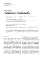
Figure 2: Bit rate as a function of the synchronisation delay Δ for ADSL downstream starting at tones 38 to 255, when the samples of CSA
loopare(a)CSALoopno.1,(b)CSALoopno.2,(c)CSALoopno.4,and(d)CSALoopno.5.
The PTEQ output x
k,n
can be specified as follows:
x
k,n
= p
H
n
·
⎡
⎣
I
T−1
0 −I
T−1
0 F
N
(n,:)
⎤
⎦


 
F
n
·y,(5)
= p
H
n
· y
k,n
,(6)
where
p
n
is the T-tap complex-valued PTEQ vector for tone
n.TheF
n
is a (T −1) ×(N + T −1) matrix [4]. The F
N
(n,:)
is the nth row of F
N
. By using the sliding DFT, the first
block row of matrix F
n
in (5) extracts the difference terms,
while the last row corresponds to the usual DFT operation as
detailed in [4, 10]. The vector y is of channel output samples
asdescribedin(1). The
y
k,n

is the sliding DFT output for tone
n at symbol k.
4. A Bit Rate Maximising Per-Tone Equalisation
In this section, we introduce the BM-PTEQ criterion with an
exact subchannel SNR model. In the derivation of the cost
EURASIP Journal on Advances in Signal Processing 5
Bit rate (bps)
0
2
4
6
8
10
12
14
×10
6
CSA loop
12345678
ABM-TEQ (RLM)
BM-TEQ
ABM-PTEQ (iQRRLM)
BM-PTEQ (MMSE)
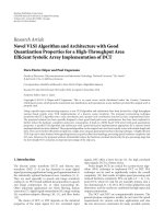
Figure 3: The bit rate performance of the BM-TEQ [11], adaptive
RLM-based BM-TEQ (ABM-TEQ) [12], proposed MMSE-based
BM-PTEQ, and proposed adaptive iQRRLM-based BM-PTEQ
(ABM-PTEQ) for all CSA loop nos. 1–8 at starting tones 38 to 255
downstream ADSL when fixed Δ
= 45.
function of BM-PTEQ, we start from the bit rate expression

as given in [14]. The total number of bits transmitted in one
DMT-symbol is defined by
b
PTEQ
=

n∈N
d
log
2

1+
SNR
n
Γ
n

,
(7)
where N
d
is the range of active tones, and SNR
n
denotes the
SNR on tone n. The constant Γ
n
is a function of the desired
probability of error, coding gain, and system margin. We
notice that an integer number of bits is allocated to optimise
the transmit power per tone after equalisation.

4.1. An Exact Subchannel SNR Model. For the BM-PTEQ
criterion to be derived, it is important to define the
dependence of the subchannel SNR on PTEQs. The SNR on
tone n can be written as
SNR
n
=
ε
s,n
ε
e,n
,
(8)
where ε
s,n
is the desired received signal energy on tone n,
and ε
e,n
is the energy in the error signal on tone n at the
FEQ output. The signal energy portions ε
s,n
and ε
e,n
in
the subchannel SNR model (8) are determined at the FFT
outputs, as assumed in [14, 15].
Following [16, 17], the PTEQ output on tone n can be
written as
p
H

n
y
k,n
= β
n
x
k,n
+

i
c
n
+

i
η
n
  
η
n
,
(9)
where the
p
n
is the complex PTEQ vector on tone n,andy
k,n
is the nth sliding DFT output vector for tone n at symbol
k.Theβ
n

x
k,n
is a scaled version of the transmitted frequency-
domain DMT-symbol
x
k,n
. The error η
n
is the sum of residual
ISI/ICI

i
c
n
and noise

i
η
n
at the nth PTEQ output. When the
scalar β
n
in (9) is equal to 1, the desired signal component
at the PTEQ output is unbiased, in case of unconstrained
MMSE PTEQ
p
∗,n
as
p
∗,n

=
E


y
H
k,n
x
k,n

E


y
H
k,n
y
k,n

. (10)
With MMSE PTEQ, the desired signal energy ε
s,n
=
E{|x
k,n
|
2
} is equal to σ
2
x

n
. The error energy ε
e,n
in (8)is
the mean square error E
{|η
n
|
2
} at the PTEQ output. It
takes residual ISI/ICI

i
c
n
and all external noise

i
η
n
sources
into account. The ratio of signal energy E
{|x
k,n
|
2
} over the
estimated error energy E
{|η
n

|
2
} yields an estimated SNR on
tone n needed in the bit rate calculation. So the SNR in
(8) is suitable to calculate the transmitted power allocation
scheme.
Therefore, the exact subchannel SNR model (8)canbe
rewritten as
SNR
max
n
=
ε
s,n
ε
e,n
=
E




x
k,n


2

E





η
n


2

=
σ
2
x
n
E





x
k,n
− p
H
∗,n
y
k,n




2

.
(11)
Introducing the compact notation for the 1
× T correla-
tion vectors

xy
n
and T ×T matrix

2
y
n
as

xy
n
= E


x
∗
k,n
y
k,n

, (12)
H


xy
n
= E


y
H
k,n
x
k,n

, (13)
2

y
n
= E


y
H
k,n
y
k,n

, (14)
and expanding the denominator of (11)gives
E





η
n


2

=
E





x
k,n
− p
H
∗,n
y
k,n



2

=
σ

2
x
n
− p
∗,n

xy
n
−p
H
∗,n
H

xy
n
+



p
∗,n


2
2

y
n
= σ
2

x
n
⎛
⎜
⎝
σ
2
x
n

2
y
n




xy
n



2
−1
⎞
⎟
⎠
,
(15)
where

p
∗,n
is the unconstrained MMSE PTEQ as defined in
(10).
6 EURASIP Journal on Advances in Signal Processing
We obtain a compact maximum SNR model SNR
max
n
by
replacing (15)in(11)as
SNR
max
n
=
σ
2
x
n
σ
2
x
n

σ
2
x
n

2
y

n
/




xy
n



2
−1

=




xy
n



2
σ
2
x
n


2
y
n
−




xy
n



2
=




xy
n



2

σ
2
x
n


2
y
n


1 −




xy
n



2
/σ
2
x
n

2
y
n

=
ρ
2
n

1 − ρ
2
n
,
(16)
with
ρ
2
n
=




xy
n



2
σ
2
x
n

2
y
n
, (17)
where ρ

2
n
is a squared normalised correlation function of
FFT output
y
k,n
and x
k,n
at the PTEQ output. We note that
the SNR
max
n
in (16) is an exact (maximum) subchannel SNR
model per tone at the PTEQs outputs, which is achieved by
using the MMSE PTEQ
p
∗,n
in (10) as described in [4]. So
this BM-PTEQ design criterion will be defined by means of
the unconstrained MMSE PTEQ
p
∗,n
asgivenin(10). This
will be used to maximise the bit rate capacity with regard to
an integer number of bits allocation as given in (7).
4.2. The BM-PTEQ Cost Function. With the use of (7)and
(16), the BM-PTEQ cost function criterion is the solution of
arg max
p
∗,n

b
max
PTEQ
= arg max
p
∗,n

n∈N
d
log
2

1+
SNR
max
n
Γ
n

=
arg max
p
∗,n

n∈N
d
log
2

1+

ρ
2
n
Γ
n

1 − ρ
2
n


=
arg max
p
∗,n

n∈N
d
log
2

Γ
n

1 − ρ
2
n

+ ρ
2

n
Γ
n

1 − ρ
2
n


=
arg max
p
∗,n

n∈N
d
log
2

Γ
n
+
(
1 − Γ
n
)
ρ
2
n
Γ

n

1 − ρ
2
n


.
(18)
By rearranging (10)intermsofcompactnotationin(13)
and (14), the unconstrained MMSE PTEQ
p
∗,n
is given as
p
∗,n
=

H
xy
n

2
y
n
,
(19)
and the squared normalised correlation parameter ρ
2
n

in (17)
is rewritten as
ρ
2
n
=

xy
n

H
xy
n
σ
2
x
n

2
y
n
.
(20)
Therefore, the BM-PTEQ cost function using the uncon-
strained MMSE PTEQs
p
∗,n
in (19) when considering the
maximum subchannel SNR at FEQs outputs in (16)is
introduced as

arg max
p
∗,n
b
max
PTEQ
= arg max
p
∗,n

n∈N
d
log
2
Γ
n
+
(
1 − Γ
n
)


xy
n

H
xy
n
/σ

2
x
n

2
y
n

Γ
n

1 −

xy
n

H
xy
n
/σ
2
x
n

2
y
n

=
arg max

p
∗,n

n∈N
d
log
2
Γ
n
σ
2
x
n
+ p
∗,n

xy
n
−p
∗,n
Γ
n

xy
n
Γ
n
σ
2
x

n
− p
∗,n
Γ
n

xy
n
= arg max
p
∗,n

n∈N
d
log
2
Γ
n

σ
2
x
n

+
(
1 − Γ
n
)



p
H
∗,n

2
y
n
p
∗,n

Γ
n

σ
2
x
n
− p
H
∗,n

2
y
n
p
∗,n

=
arg max

p
∗,n

n∈N
d
log
2
p
∗,n
Γ
n
p
H
∗,n
+p
∗,n
ρ
2
n
p
H
∗,n
−p
∗,n
Γ
n
ρ
2
n
p

H
∗,n
p
∗,n
Γ
n
p
H
∗,n
−p
∗,n
Γ
n
ρ
2
n
p
H
∗,n
= arg max
p
∗,n

n∈N
d
log
2
p
∗,n


Γ
n

1 − ρ
2
n

+ ρ
2
n

p
H
∗,n
p
∗,n

Γ
n

1 − ρ
2
n


p
H
∗,n
=arg max
p

∗,n

n∈N
d
log
2
p
∗,n

Γ
n

σ
2
x
n

2
y
n
−g

+ g


p
H
∗,n
p
∗,n


Γ
n

σ
2
x
n

2
y
n
−g


p
H
∗,n
= arg max
p
∗,n

n∈N
d
log
2
p
∗,n
A
n

p
H
∗,n
p
∗,n
B
n
p
H
∗,n
,
(21)
where g represents

x y
n

H
x y
n
and A
n
and B
n
depend on the
second order statistics information σ
2
x
n
,


2
y
n
and

xy
n
A
n
= Γ
n
⎛
⎝
σ
2
x
n
2

y
n
−

x y
n
H

x y
n

⎞
⎠
+

x y
n
H

x y
n
,
B
n
= Γ
n
⎛
⎝
σ
2
x
n
2

y
n
−

x y
n
H


x y
n
⎞
⎠
(22)
Clearly, (21) has the exact form for the BM-TEQ solution
of [11] with only a trivial interchange of the maximisation
and minimisation operations for the argument. Therefore,
the solution to achieve BM-PTEQ
p
∗,n
can be also achieved
with the same methodology for the bit rate maximising TEQ
of [11]. This leads us to the crucial point that, given the
proven superior performance of PTEQ over TEQ [13], the
BM-PTEQ will always continue to do better than the BM-
TEQ of [11] in the sense of bit rate maximising performance.
Proposition 1. The bit rate performance of the BM-PTEQ is
greater than or equal to that of the BM-TEQ,
b
max
PTEQ
≥ b
max
TEQ
, (23)
where b
max
TEQ

represents the maximum bit rate achievable from
the BM-TEQ of [11].
EURASIP Journal on Advances in Signal Processing 7
5. An Adaptive Bit Rate Maximising
Per-Tone Equalisation
In Section 5.1, we introduce the constrained nonlinear
exponentially weighted cost function for the complex-valued
PTEQ. This criterion is translated with the deterministic
approach to accomplish the maximum number of bits per
DMT-symbol. With this nonlinear criterion in Section 5.1,
we introduce an adaptive BM-PTEQ algorithm based on
RLM algorithm in Section 5.2.
5.1. The Constrained Nonlinear BM-PTEQ Cost Function.
This criterion follows from the constrained nonlinear opti-
misation problem as described in [12], which is modified for
the complex-valued PTEQs criterion as
max
p
∗,n

n∈N
d
log
2

1+
SNR
n
Γ
n


,
(24)
with
SNR
n
=
σ
2
x
n
E





x
k,n
− p
H
∗,n
y
k,n



2

,

(25)
subject to
p
∗,n
=
E


y
H
k,n
x
k,n

E


y
H
k,n
y
k,n

=

H
x y
n

2

y
n
, ∀n ∈ N
d
, (26)
where
x
k,n
is the kth transmitted DMT-symbol on tone n.
The σ
2
x
n
= E{|x
k,n
|
2
} is a variance and y
k,n
is the kth
unequalised T
× 1 symbol vector after sliding DFT at tone
n. We aim to maximise the number of bits per DMT-symbol
in (24) subject to the unconstrained MMSE PTEQ
p
∗,n
in
(26) with the subchannel SNR on n tone in (25).
A constrained optimisation criterion is typically restated
as a cost minimisation

J


p
∗,n

=

n∈N
d
log
2

1+
SNR
n
Γ
n

.
(27)
By means of the least squares criterion, the gradient of
(27)withrespecttoPTEQs
p
∗,n
can be rewritten compactly
with an exponentially weighted over K DMT-symbols as (see
also in the appendix)
∇
p

∗,n
J =

n∈N
d
K

k=1
λ
K−k
γ
k,n
y
H
k,n
e
∗
k,n
,
(28)
with
γ
k,n
=
SNR
2
n
σ
2
x

k,n
(
Γ
n
+SNR
n
)
,
e
k,n
= E





x
k,n
− p
H
∗,n
y
k,n




,
(29)
where

γ
k,n
is a tone-dependent weight and e
k,n
is the error on
tone n at symbol k.
Hence,
γ
k,n
is replaced by an instantaneous a priori esti-
mate based on the previous parameter tap-weight estimate
vector
p
k−1,n
on tone n at symbol k − 1. Consequently,
the tone-dependent weight estimate
γ
k,n
at tone n for each
symbol k is given as
γ
k,n
=

SNR
2
k,n
σ
2
x

k,n

Γ
n
+

SNR
k,n

,
(30)
where

SNR
k,n
=
σ
2
x
n




x
k,n
− p
H
k
−1,n

y
k,n



2
.
(31)
The gradient in (28) is also applied to the nonlinear
weighted problem with varying weight estimate
γ
k,n
and the
instantaneous estimate SNR at each symbol k for n tone

SNR
k,n
. We note that the denominator of

SNR
k,n
in (31)
is equal to the MSE with the previous tap-weight estimate
vector
p
k−1,n
at the PTEQ output.
Therefore, a constrained nonlinear exponentially weight-
ed least squares cost function for the complex-valued PTEQ
tap-weight estimate vector

p
k,n
is defined as
J
NL


p
k,n

=

n∈N
d
1
2
K

k=1
λ
K−k
γ
k,n



e
k,n



2
, (32)
e
k,n
= x
k,n
− p
H
k
−1,n
y
k,n
, (33)
where
e
k,n
is the a priori estimate error at each DMT-
symbol. With the nonlinear cost function in (32), an adaptive
algorithm introduced in Section 5.2 can achieve the same
performance as the BM-PTEQ cost function in (21)with
these approximations in (30)and(31).
5.2. An Adaptive BM-PTEQ Algorithm. In this section, we
introduce the methodology in solving the nonlinear cost
function in (32) recursively at each symbol k based on an
adaptive recursive Levenberg-Marquardt (RLM) algorithm
updating of T
× 1 PTEQ tap-weight vector p
k,n
at tone n
for n

∈ N
d
. The iterative Levenberg Marquadt (LM) method
is classical and well-known strategies for solving nonlinear
batch optimisation problems. The recursive LM is definitely
modified for adaptively solving nonlinear problems by earlier
algorithms as the recursive identification system presented in
[18] and neural network for nonlinear adaptive filter training
described in [19].
The constrained nonlinear exponentially least squares
cost criterion in (32) for a complex-valued tap-weight
estimate PTEQ
p
k,n
at DMT-symbol k on tone n is defined
as
J

p
k,n

=
1
2
K

k=1
λ
K−k
γ

k,n



e
k,n


2
,
(34)
where
γ
k,n
is a scalar of tone-dependent weight estimate
asgivenin(30)and
e
k,n
is the a priori estimate error as
described in (33).
8 EURASIP Journal on Advances in Signal Processing
Following [18], a tap-weight estimate PTEQ
p
k,n
can be
obtained at each DMT-symbol k as
p
k,n
= p
k−1,n

+
ˇ
R
−1
k,n
g
k,n
,
(35)
where the gradient estimate
g
k,n
is derived by differentiating
the cost function in (34)withrespectto
p
k,n
in (35)as
g
k,n
=∇
p
k,n
J = γ
k,n
y
H
k,n
e
∗
k,n

.
(36)
Based on LM method [20], the regularised approximation
Hessian
ˇ
R
k,n
is reformed as
ˇ
R
k,n
=
K

k=1
λ
K−k


γ
k,n
y
k,n
y
H
k,n

+ δ
k,n
diag


R
k,n


, (37)
R
k,n
=
K

k=1
λ
K−k
γ
k,n
y
k,n
y
H
k,n
, (38)
where R
k,n
is the approximation Hessian for the complexed
PTEQ. The δ
k,n
is the regularisation parameter at symbol k
[19], in which this algorithm ensures the stability by taking
the changing of the approximation Hessian over symbol into

account. Hence, the regularised approximation Hessian
ˇ
R
k,n
is regularised for stability reason by the second term in (37).
With the recursion method, the tap-weight estimate
PTEQ vector
p
k,n
is updated as
p
k,n
= p
k−1,n
+
(
1 − λ
)

R
−1
k,n
g
k,n
,
(39)
where

R
k,n

= λ

R
k−1,n
+
(
1 − λ
)


γ
k,n
y
k,n
y
H
k,n

+δ
k,n
diag


γ
k,n
y
k,n
y
H
k,n


,
(40)
where λ is the forgetting-factor, 0 <λ<1. The regularised
approximation Hessian
ˇ
R
k,n
in (37) is replaced by an
exponentially weighted estimate approximation Hessian

R
k,n
in (40).
5.2.1. The Modified Inverse Regularised Approximation Hes-
sian Matrix. Unfortunately, the matrix inversion lemma
cannot be used directly on the updating approximation
Hessian

R
k,n
in (40). So, we rearrange

R
k,n

R
k,n
= λ


R
k−1,n
+
(
1 − λ
)
γ
k,n


y
k,n
y
H
k,n

+δ
k,n
diag


y
k,n
y
H
k,n

,
(41)
by adding the ϕ

k,n
matrix and ψ
k,n
matrix into (41)(The
matrix inversion lemma.LetA and B be two positive definite
M-by-M matrices related by A
= B
−1
+ C ·D
−1
· C
H
,where
D is a positive definite N-by-M matrix and C is an M-by-N
matrix. We may express the inverse of the matrix A by A
−1
=
B −BC(D + C
H
BC)
−1
C
H
B.) .
We then introduce how to define

R
k,n
as


R
k,n
= λ

R
k−1,n
+
(
1 − λ
)
γ
k,n

ψ
k,n
ϕ
k,n
ψ
H
k,n

, (42)
where
ψ
k,n
=
⎡
⎣

y

k,n
0
T

I
⎤
⎦
=
⎡
⎢
⎢
⎢
⎢
⎢
⎢
⎢
⎢
⎢
⎢
⎢
⎢
⎣

y
(1)
k,n
00··· 0
y
(2)
k,n

10··· 0
y
(3)
k,n
01··· 0
.
.
.
.
.
.
.
.
.
.
.
.
.
.
.
y
(T)
k,n
00··· 1
⎤
⎥
⎥
⎥
⎥
⎥

⎥
⎥
⎥
⎥
⎥
⎥
⎥
⎦
, (43)
Υ
k,n
= δ
k,n
diag


y
k,n
y
H
k,n

=
⎡
⎣
Υ
11
0
T
0 Υ

22
⎤
⎦
, (44)
ϕ
k,n
=
⎡
⎣
1 0
T
0 Υ
22
⎤
⎦
, (45)
where ψ
k,n
denotes the T × T matrix. The Υ
22
is the (T −
1) × (T − 1) block diagonal matrix. The size of zero vector
0 is of 1
× (T − 1), and the size of the identity matrix

I is
of (T
− 1) × (T − 1). Notice that Υ
k,n
in (44)andϕ

k,n
in
(45) are the T
× T block diagonal matrices. Hence, the ϕ
k,n
is nonsingular, if and only if its inverse exists [21]. With the
approximation Hessian

R
k,n
assumed to be positive definite
and therefore nonsingular, we can apply the matrix inversion
lemma to the modified approximation Hessian

R
k,n
in (42)
instead of

R
k,n
in (41).
We make the following identifications as A
=

R
k,n
,
B
−1

= λ

R
k−1,n
, C = ψ
k,n
, D
−1
= (1 − λ)γ
k,n
ϕ
k,n
.By
substituting these definitions in the matrix inversion lemma,
we then obtain the following recursive equation for the
inverse of the modified approximation Hessian

R
k,n
as

R
−1
k,n
= λ
−1

R
−1
k

−1,n
−λ
−1

R
−1
k
−1,n

K
k,n
ψ
H
k,n
, (46)

K
k,n
=
λ
−1

R
−1
k
−1,n
ψ
k,n

(1 −λ)

−1
γ
−1
k,n
ϕ
−1
k,n

+

λ
−1
ψ
H
k,n

R
−1
k
−1,n
ψ
k,n

, (47)
where
γ
k,n
is a scalar of tone-dependent weight estimate as
givenin(30).
Consequently, the tap-weight estimate PTEQ vector

p
k,n
can be computed as
p
k,n
= p
k−1,n
+
(
1 − λ
)

R
−1
k,n
g
k,n
,
(48)
where

R
−1
k,n
is introduced above in (46)andg
k,n
is the gradient
estimate in (36).
5.2.2. An Adaptive Inverse Square-Root Recursive Levenberg-
Marquardt (iQR-RLM) Algorithm. We consider the Givens

rotation-based adaptive inverse square-root (QR) algorithm.
An adaptive inverse QR algorithm is a QR decomposition-
based recursive least squares (QR-RLS) algorithm that is
designed to obtain explicit weight extraction by work-
ing directly with the incoming data matrix via the QR
decomposition [22]. Accordingly, the QR-RLS algorithm is
numerically more stable than the standard RLS algorithm
[23].
EURASIP Journal on Advances in Signal Processing 9
Notice that the modified inverse approximation Hessian

R
−1
k,n
in (46) is also derived in a similar fashion with the
inverse correlation Φ
−1
k,n
of RLS algorithm as described in
[23]. Hence, the form of

R
−1
k,n
in (46) of RLM algorithm is
similar to the inverse correlation Φ
−1
k,n
of RLS algorithm. We
then introduce the Givens rotation-based adaptive inverse

QR algorithm, which can be applied for

R
−1
k,n
of RLM
algorithm for computing the PTEQ tap-weight estimate
p
k,n
at symbol k for tone n ∈ N
d
.
For convenience of computation, let
D
k,n


R
−1
k,n
,
z
k,n
=

(
1
−λ
)
−1

γ
−1
k,n
ϕ
−1
k,n

+

λ
−1
ψ
H
k,n
D
k−1,n
ψ
k,n

.
(49)
Using these definitions in (49), we may rewrite

R
−1
k,n
(46)
as
D
k,n

= λ
−1
D
k−1,n
−λ
−1
D
k−1,n
ψ
k,n
z
−1
k,n
ψ
H
k,n
λ
−1
D
k−1,n
.
(50)
There are 4-matrix terms that constitute the right-hand
side of (50), we may introduce the 2
×2blockmatrixG as
G
=
⎡
⎣
z

k,n
λ
−1
ψ
H
k,n
D
k−1,n
λ
−1
D
k−1,n
ψ
k,n
λ
−1
D
k−1,n
⎤
⎦
. (51)
We then redefine the block matrix G in (51) using the
Cholesky factorisation as
G
= AA
H
,
A =
⎡
⎣

(1 −λ)
−1/2
γ
−1/2
k,n
ϕ
−1/2
k,n
λ
−1/2
ψ
H
k,n
D
1/2
k
−1,n
0 λ
−1/2
D
1/2
k
−1,n
⎤
⎦
,
(52)
where 0 is the null vector, the prearray
A is an upper
triangular matrix and D

k−1,n
indicates with its factor
D
k−1,n
= D
1/2
k
−1,n
D
H/2
k
−1,n
.
(53)
We may set the prearray
A to resulting the postarray
B transformation for iQR-RLM algorithm using the matrix
factorisation lemma as
AΘ = B,
⎡
⎣
(1 −λ)
−1/2
γ
−1/2
k,n
ϕ
−1/2
k,n
λ

−1/2
ψ
H
k,n
D
1/2
k
−1,n
0 λ
−1/2
D
1/2
k
−1,n
⎤
⎦
Θ
=
⎡
⎣
z
1/2
k,n
0
T

K
k,n
z
1/2

k,n
D
1/2
k,n
⎤
⎦
,
(54)
where Θ is a unitary rotation and

K
k,n
is described in (47)
( The matrix factorisation lemma.GivenanyA and B n
×
m matrices with dimention n ≤ m, this lemma states by
following [23]asAΘΘ
H
A
H
= BB
H
, if and only if, there exists
a unitary matrix Θ such that AΘ
= B and ΘΘ
H
= I.) .
We note that D
1/2
k,n

in the right-hand side of (54) is the
lower triangular matrix. In virtue of the product of square-
root matrix its Hermitian transpose
D
k,n
= D
1/2
k,n
D
H/2
k,n
(55)
is always nonnegative matrix as derived in [24].
Therefore, the tap-weight estimate PTEQ vector
p
k,n
based on iQR-RLM algorithm can be performed
p
k,n
= p
k−1,n
+
(
1 − λ
)
D
k,n
g
k,n
,

(56)
where D
k,n
is defined in (55)andg
k,n
is the gradient estimate
in (36).
5.2.3. The Adaptive Regularisation Parameter. Both the con-
vergence rate and stability are affected by a suitable choice
of the regularisation parameter δ
k,n
such that a small δ
k,n
could cause the RLM algorithm to be unstable, while a
large δ
k,n
could deduce slow convergence [18]. So the
parameter δ
k,n
should be adapted during convergence. An
adaptive regularisation parameter algorithm based on the
instantaneous estimates of the predicted and actual cost
criterion reduction is proposed in [19]. Hence, we apply this
algorithm for an adaptive iQR-RLM algorithm as explained
below.
Following [19], the predicted instantaneous cost reduc-
tion
r
p
k,n

of the criterion in (34) for each update of iQRRLM-
based algorithm (56)iscomputedas
r
p
k,n
=
(
1
−λ
)


γ
k,n
y
H
k,n
e
∗
k,n

H
D
k,n


γ
k,n
y
H

k,n
e
∗
k,n

, (57)
e
k,n
= x
k,n
− p
H
k
−1,n
y
k,n
, (58)
where
γ
k,n
is a scalar of tone-dependent weight estimate as
givenin(30). The error
e
k,n
is a priori estimate error, and D
k,n
is the inverse of modified approximation Hessian in (55).
The actual instantaneous cost reduction
r
a

k,n
is deter-
mined by using a priori estimate error
e
k,n
in (58)anda
posteriori estimate error

ξ
k,n
as
r
a
k,n
= γ
k,n




e
k,n


2
−





ξ
k,n



2

,

ξ
k,n
= x
k,n
− p
H
k,n
y
k,n
.
(59)
Then, the values for δ
k,n
can be adapted using the
following criterion.
(i) Increase δ
k−1,n
by a factor of α if r
a
k,n
/r

p
k,n
is smaller
than a threshold ζ.
(ii) Decrease δ
k−1,n
by a factor of 1/α if r
a
k,n
/r
p
k,n
is larger
than a threshold 1
−ζ.
The adaptive regularisation parameter δ
k,n
method is sum-
marised as
δ
k,n
=
⎧
⎪
⎪
⎪
⎪
⎪
⎨
⎪

⎪
⎪
⎪
⎪
⎩
α · δ
k−1,n
,ifr
a
k,n
<ζ r
p
k,n
,
1
α
·δ
k−1,n
,ifr
a
k,n
>
(
1 − ζ
)
r
p
k,n
,
δ

k−1,n
, otherwise,
(60)
where 0 <ζ<0.5 and a typical value is of 0.25.
Therefore, the iQR-RLM algorithm for BM-PTEQ using
adaptive regularisation method is summarised as described
in Algorithm 1.
10 EURASIP Journal on Advances in Signal Processing
Starting with the soft-constrained initialisation as: p(0) = 0
For n
∈ N
d
, n = 1, 2, , compute.
for k
= 1,2, , K
(1) To arrange the block diagonal matrices ψ
k,n
, Υ
k,n
and ϕ
k,n
as:
ψ
k,n
=
⎡
⎢
⎢
⎢
⎢

⎢
⎢
⎢
⎢
⎢
⎢
⎢
⎢
⎣

y
(1)
k,n
00··· 0
y
(2)
k,n
10··· 0
y
(3)
k,n
01··· 0
.
.
.
.
.
.
.
.

.
.
.
.
.
.
.
y
(T)
k,n
00··· 1
⎤
⎥
⎥
⎥
⎥
⎥
⎥
⎥
⎥
⎥
⎥
⎥
⎥
⎦
,
Υ
k,n
= δ
k,n

diag{y
k,n
y
H
k,n
}=
⎡
⎣
Υ
11
0
0 Υ
22
⎤
⎦
,
ϕ
k,n
=
⎡
⎣
1 0
0 Υ
22
⎤
⎦
,
where
y
k,n

=


y
(1)
k,n
y
(2)
k,n
··· y
(T)
k,n

T
.
(2) To compute

SNR
k,n
and γ
k,n
as:

SNR
k,n
=
σ
2
x
n

|x
k,n
− p
H
k
−1,n
y
k,n
|
2
,
γ
k,n
=

SNR
2
k,n
σ
2
x
n
(Γ
n
+

SNR
k,n
)
.

(3) To compute D
k,n
as:
A =
⎡
⎣
(1 −λ)
−1/2
γ
−1/2
k,n
ϕ
−1/2
k,n
λ
−1/2
ψ
H
k,n
D
1/2
k
−1,n
0 λ
−1/2
D
1/2
k
−1,n
⎤

⎦
,
AΘ =
⎡
⎣
B
11
b
12
b
21
B
22
⎤
⎦
,whereΘ is a unitary rotation,
D
k,n
= B
22
B
H
22
.
(4) To compute
p
k,n
as:
p
k,n

= p
k−1,n
+(1−λ)D
k,n
g
k,n
,
where
g
k,n
= γ
k,n
y
H
k,n
e
∗
k,n
,
e
k,n
= x
k,n
− p
H
k
−1,n
y
k,n
.

(5) To compute δ
k,n
as:
δ
k,n
=
⎧
⎪
⎪
⎪
⎪
⎪
⎨
⎪
⎪
⎪
⎪
⎪
⎩
α ·δ
k−1,n
if r
a
k,n
<ζr
p
k,n
,
1
α

·δ
k−1,n
if r
a
k,n
> (1 −ζ)r
p
k,n
,
δ
k−1,n
otherwise,
where
r
p
k,n
= (1 −λ)[γ
k,n
y
H
k,n
e
∗
k,n
]
H
D
k,n
[γ
k,n

y
H
k,n
e
∗
k,n
],
r
a
k,n
= γ
k,n
{|e
k,n
|
2
−|

ξ
k,n
|
2
},

ξ
k,n
= x
k,n
− p
H

k,n
y
k,n
.
end
end
Algorithm 1: Summary of the proposed adaptive iQRRLM-based BM-PTEQ.
EURASIP Journal on Advances in Signal Processing 11
6. Simulation Results
In this section, we performed transmission simulations for
the ADSL downstream including AWGN and NEXT over
the entire test channel. The used tones were starting at
tones 38 to 255, and the unused tones were set to zero.
The bit allocation calculation requires an estimate of SNR
on tone n
∈ N
d
, when the noise energy is estimated after
per-tone equalisation. The carrier serving area (CSA) loop
nos. 1–8 were used for the test channel, which comprises 512
coefficients of CIR. The length of CP (ν) was 32. The SNR gap
of 9.8 dB, the coding gain of 4.2 dB, the noise margin of 6 dB,
and the input signal power of
−40 dBm/Hz were used for all
active tones. The AWGN with a power of
−140 dBm/Hz and
NEXT coming from 12 ADSL disturbers were included. All
simulations were done for T
= 32, f
s

= 2.208 MHz, and
N
= 512.
We compare the proposed MMSE-based BM-PTEQ with
iterative method, the proposed adaptive BM-PTEQ with
adaptive iQRRLM-based design, with the RLM-based PTEQ
approach [6], with other BM-TEQ such as BM-TEQ with
iterative scheme [11] and with the recursive method [12].
The BM-TEQ was initialised with w
= [1 0 ··· 0]
T
,as
presentedin[11]. The proposed iQRRLM-based BM-PTEQ
can be computed with the soft-constrained initialisation. The
regularisation parameter δ
k
of adaptive RLM-based PTEQ
[6], adaptive RLM-based BM-TEQ [12], and proposed adap-
tive iQRRLM-based BM-PTEQ were initialised at δ
0
= 10
−3
for all active tones. The forgetting-factor λ of the adaptive
RLM-based PTEQ [6], the RLM-based adaptive BM-TEQ
(ABM-TEQ) [12], and the proposed adaptive iQRRLM-
based BM-PTEQ (ABM-PTEQ) were increased from λ
=
0.95 during the first 150 update-symbols to λ = 0.99 for the
remaining updated symbols. The adaptation parameter α of
δ

k
of the proposed iQRRLM-based adaptive BM-PTEQ was
fixed at α
= 2.
Figure 1 depicts that the learning curves of bit rate
convergence of all adaptive algorithms as a function of
the number of updated DMT-symbols for the samples of
CSA loop no. 1, no. 2, no. 4 and no. 5. The proposed
iQR-RLM adaptive BM-PTEQ (ABM-PTEQ) is compared
with the RLM-based adaptive BM-TEQ (ABM-TEQ) [12].
The bit rate of the RLM-based adaptive BM-TEQ [12]
curves closely to reach the maximum bit rate of BM-TEQ
[11]. Meanwhile, the learning curve of proposed adaptive
BM-PTEQ with iQRRLM-based algorithm converges nearly
to the truly MMSE-based BM-PTEQ. Approximately, 100
updated symbols are appeared to converge to steady-state
condition for the proposed iQRRLM-based adaptive BM-
PTEQ. The curve of proposed iQRRLM-based adaptive
BM-PTEQ has slower convergence than the RLM-based
adaptive BM-TEQ. The adaptive RLM-based PTEQ has
the slowest convergence. In [11], the performance of BM-
TEQ has shown closely to PTEQ and the learning curve
of adaptive RLM-based BM-TEQ compared with adaptive
RLM-based PTEQ [6] in both these figures reveal to
confirm.
Figure 2 illustrates the bit rate as a function of syn-
chronisation delay Δ of T-tap complexed equalisers for the
samples of CSA loop no. 1, no. 2, no. 4, and no. 5, when
the numbers of taps of equalisers equal 32 (T
= 32). The

proposed BM-PTEQ and ABM-PTEQ are compared with
the BM-TEQ [11] design. It is noticed that the proposed
ABM-PTEQ performance has the same direction with the
proposed BM-PTEQ design along the number of increasing
delay for all samples of CSA loop. The performance of
the BM-TEQ confirms that its bit rate has been smooth
as a function of delay, as presented in [11]. The proposed
ABM-PTEQ and BM-PTEQ appear to give higher bit rate
than BM-TEQ design for a given range of synchronisation
delay.
Figure 3 reveals the bit rate performance of the proposed
MMSE-based BM-PTEQ and adaptive iQRRLM-based BM-
PTEQ (ABM-PTEQ) for all CSA loop nos. 1–8 at starting
tones 38 to 255 ADSL downstream when the fixed delay
equals 45 (Δ
= 45). The performance of proposed ABM-
PTEQ is compared with BM-TEQ [11]andadaptiveRLM-
based BM-TEQ (ABM-TEQ) [12]. It is shown that the
proposed ABM-PTEQ is similar to the performance of BM-
PTEQ approach. The bit rate of proposed ABM-PTEQ can be
improved as compared to the BM-TEQ and the ABM-TEQ
design.
7. Conclusion
In this paper, we present the BM-PTEQ design with the
nonlinear bit rate maximising cost function. The proposed
BM-PTEQ cost function is derived from the exact subchan-
nel SNR model at the FEQ outputs. Since, the solution
to achieve the BM-PTEQ criterion is exactly the same
form of that of the BM-TEQ, we conclude that the BM-
PTEQ can always perform better than or equal to the

BM-TEQ in the sense of bit rate maximising performance.
For achievable BM-PTEQ in practice, we then introduce
the methodology of adaptive inverse-QR RLM-based BM-
PTEQ design by the nonlinear bit rate maximising cost
criterion. The proposed BM-PTEQ and iQRRLM-based
ABM-PTEQ can ensure the performance of maximum bit
rate. Simulation results with several ADSL parameters show
that the proposed BM-PTEQ and iQRRLM-based ABM-
PTEQ are able to improve superior bit rate performance as
compared with BM-TEQ and ABM-TEQ design for all CSA
loop.
Appendix
The constrained optimisation criterion is given as
J

p
∗,n

=

n∈N
d
log
2

1+
SNR
n
Γ
n


.
(A.1)
12 EURASIP Journal on Advances in Signal Processing
The derivation of the gradient of (A.1)withrespecttoPTEQ
p
∗,n
is
∇
p
∗,n
J =

n∈N
d
∂
∂p
∗,n

log
2

1+
SNR
n
Γ
n

=


n∈N
d

Γ
n
Γ
n
+SNR
n

∂
∂p
∗,n

1+
SNR
n
Γ
n

=

n∈N
d

σ
2
x
n
Γ

n
+SNR
n


y
H
k,n
e
∗
k,n

E





x
k,n
− p
H
∗,n
y
k,n



2


2
=

n∈N
d
SNR
2
n
σ
2
x
k,n
(
Γ
n
+SNR
n
)
y
H
k,n
e
∗
k,n
=

n∈N
d
γ
k,n

y
H
k,n
e
∗
k,n
,
(A.2)
where SNR
n
is the SNR on tone n,andγ
k,n
is a tone-
dependentweightatsymbolk on tone n
SNR
n
=
σ
2
x
n
E





x
k,n
− p

H
∗,n
y
k,n



2

,
γ
k,n
=
SNR
2
n
σ
2
x
n
(
Γ
n
+SNR
n
)
,
e
k,n
= E






x
k,n
− p
H
∗,n
y
k,n




.
(A.3)
The gradient in (A.2) of the constrained optimisation
criterion in (A.1)withrespecttoPTEQ
p
∗,n
can be expressed
with the exponentially weighted over K DMT-symbols as
∇
p
∗,n
J =

n∈N

d
K

k=1
λ
K−k
γ
k,n
y
H
k,n
e
∗
k,n
,
(A.4)
where λ is an exponential weighting factor or forgetting
factor.
Acknowledgment
This work was supported by the Shell Centennial Education
Fund, Thailand.
References
[1] R. Baldemair and P. Frenger, “A time-domain equalizer
minimizing intersymbol and intercarrier interference in DMT
systems,” in Proceedings of IEEE Global Telecommunications
Conference (GLOBECOM ’01), vol. 1, pp. 381–385, 2001.
[2] S. Sitjongsataporn and P. Yuvapoositanon, “An adaptive step-
size order statistic time domain equaliser for discrete multi-
tone systems,” in Proceedings of IEEE International Symposium
on Circuits and Systems (ISCAS ’07), pp. 1333–1336, New

Orleans, LA, USA, May 2007.
[3] T. Pollet, M. Peeters, M. Moonen, and L. Vandendorpe,
“Equalization for DMT-based broadband modems,” IEEE
Communications Magazine, vol. 38, no. 5, pp. 106–113, 2000.
[4] K. Van Acker, G. Leus, M. Moonen, O. van de Wiel, and T.
Pollet, “Per tone equalization for DMT-based systems,” IEEE
Transactions on Communications, vol. 49, no. 1, pp. 109–119,
2001.
[5] G. Ysebaert, K. Vanbleu, G. Cuypers, M. Moonen, and
T. Pollet, “Combined RLS-LMS initialization for per tone
equalizers in DMT-receivers,” IEEE Transactions on Signal
Processing, vol. 51, no. 7, pp. 1916–1927, 2003.
[6] S. Sitjongsataporn and P. Yuvapoositanon, “Recursive
Levenberg-Marquardt per-tone equalisation for discrete
multitone systems,” in Proceedings of the 3rd International
Symposium on Communications, Control, and Signal Processing
(ISCCSP ’08), pp. 1062–1066, St. Julians, Malta, March 2008.
[7] K. Van Acker, G. Leus, M. Moonen, and T. Pollet, “RLS-based
initialization for per-tone equalizers in DMT receivers,” IEEE
Transactions on Communications, vol. 51, no. 6, pp. 885–889,
2003.
[8] K. Van Acker, G. Leus, M. Moonen, and T. Pollet, “Frequency
domain equalization with tone grouping in DMT/ADSL-
receivers,” in Proceedings of the Conference Record of the Asilo-
mar Conference on Signals, Systems and Computers (Asilomar
’99), vol. 2, pp. 1067–1070, 1999.
[9] K. Vanbleu, G. Ysebaert, G. Cuypers, and M. Moonen, “Bitrate
maximizing per group equalization for DMT-based systems,”
Signal Processing, vol. 86, no. 10, pp. 2952–2965, 2006.
[10] P. K. Pandey and M. Moonen, “Resource allocation in ADSL

variable length per-tone equalizers,” IEEE Transactions on
Signal Processing, vol. 56, no. 5, pp. 2161–2164, 2008.
[11] K. Vanbleu, G. Ysebaert, G. Cuypers, M. Moonen, and K. Van
Acker, “Bitrate-maximizing time-domain equalizer design for
DMT-based systems,” IEEE Transactions on Communications,
vol. 52, no. 6, pp. 871–876, 2004.
[12] K. Vanbleu, G. Ysebaert, G. Cuypers, and G. Leus, “Adaptive
bitrate maximizing TEQ design for DMT-based systems,”
in Proceedings of IEEE International Conference on Acoustics,
Speech and Signal Processing (ICASSP ’04), vol. 4, pp. 1057–
1060, May 2004.
[13] K. Van Acker, Equalization and echo cancellation for DMT-
based DSL mode ms, Ph.D. thesis, Katholieke Universiteit
Leuven, Leuven, Belgium, 2001.
[14] N. Al-Dhahir and J. M. Cioffi, “Optimum finite-length
equalization for multicamer transceivers,” IEEE Transactions
on Communications, vol. 44, no. 1, pp. 56–64, 1996.
[15] W. Henkel and T. Kessler, “Maximizing the channel capacity of
multicarrier transmission bysuitable adaptation of the time-
domain equalizer,” IEEE Transactions on Communications, vol.
48, no. 12, pp. 2000–2004, 2000.
[16] J. M. Cioffi, G. P. Dudevoir, M. V. Eyuboglu, and G. D. Forney
Jr., “MMSE decision-feedback equalizers and coding—part I:
equalization results,” IEEE Transactions on Communications,
vol. 43, no. 10, pp. 2582–2594, 1995.
[17] E. de Carvalho and D. T. M. Slock, “Burst mode equalization:
optimal approach and suboptimal continuous-processing
approximation,” Signal Processing, vol. 80, no. 10, pp. 1999–
2015, 2000.
[18] L. Ljung and T. S

¨
oderstr
¨
om, Theory and Practice of Recursive
Identification, Cambridge, Mass, USA, MIT Press, 1983.
[19] L. S. H. Ngia and J. Sj
¨
oberg, “Efficient training of neural nets
for nonlinear adaptive filtering using a recursive Levenberg-
Marquardt algorithm,” IEEE Transactions on Signal Processing,
vol. 48, no. 7, pp. 1915–1927, 2000.
[20] W. H. Press, S. A. Teukolsky, W. T. Vetterling, and B.
P. Flannery, Numerical Recipes in C: The Art of Scientific
EURASIP Journal on Advances in Signal Processing 13
Computing, Cambridge University Press, Cambridge, UK,
1993.
[21]R.A.HornandC.R.Johnson,Matrix Analysis, Cambridge
University Press, Cambridge, UK, 1999.
[22] J. Ma, K. K. Parhi, and E. F. Deprettere, “A unified algebraic
transformation approach for parallel recursive and adaptive
filtering and svd algorithms,” IEEE Transactions on Signal
Processing, vol. 49, no. 2, pp. 424–437, 2001.
[23] S. Haykin, Adaptive Filter Theory, Prentice-Hall, Upper Saddle
River, NJ, USA, 1996.
[24] A. H. Sayed and T. Kailath, “A state-space approach to adaptive
RLS filtering,” IEEE Signal Processing Magazine,vol.11,no.3,
pp. 18–60, 1994.