báo cáo hóa học:" Research Article Robust Distributed Noise Reduction in Hearing Aids with External Acoustic Sensor Nodes" ppt

Hindawi Publishing Corporation
EURASIP Journal on Advances in Signal Processing
Volume 2009, Article ID 530435, 14 pages
doi:10.1155/2009/530435
Research Article
Robust Distributed Noise Reduction in Hearing Aids with
External Acoustic Sensor Nodes
Alexander Bertrand and Marc Moonen (EURASIP Member)
Department of Electrical Engineering (ESAT-SCD), Katholieke Universiteit Leuven, Kasteelpark Arenberg 10,
3001 Leuven, Belgium
Correspondence should be addressed to Alexander Bertrand,
Received 15 December 2008; Revised 17 June 2009; Accepted 24 August 2009
Recommended by Walter Kellermann
The benefit of using external acoustic sensor nodes for noise reduction in hearing aids is demonstrated in a simulated acoustic
scenario with multiple sound sources. A distributed adaptive node-specific signal estimation (DANSE) algorithm, that has a
reduced communication bandwidth and computational load, is evaluated. Batch-mode simulations compare the noise reduction
performance of a centralized multi-channel Wiener filter (MWF) with DANSE. In the simulated scenario, DANSE is observed not
to be able to achieve the same performance as its centralized MWF equivalent, although in theory both should generate the same set
of filters. A modification to DANSE is proposed to increase its robustness, yielding smaller discrepancy between the performance
of DANSE and the centralized MWF. Furthermore, the influence of several parameters such as the DFT size used for frequency
domain processing and possible delays in the communication link between nodes is investigated.
Copyright © 2009 A. Bertrand and M. Moonen. This is an open access article distributed under the Creative Commons
Attribution License, which permits unrestricted use, distribution, and reproduction in any medium, provided the original work is
properly cited.
1. Introduction
Noise reduction algorithms are crucial in hearing aids to
improve speech understanding in background noise. For
every increase of 1 dB in signal-to-noise ratio (SNR), speech
understanding increases by roughly 10% [1]. By using
an array of microphones, it is possible to exploit spatial
characteristics of the acoustic scenario. However, in many

classical beamforming applications, the acoustic field is
sampled only locally because the microphones are placed
close to each other. The noise reduction performance can
often be increased when extra microphones are used at
significantly different positions in the acoustic field. For
example, an exchange of microphone signals between a pair
of hearing aids in a binaural configuration, that is, one
at each ear, can significantly improve the noise reduction
performance [2–11]. The distribution of extra acoustic
sensor nodes in the acoustic environment, each having a
signal processing unit and a wireless link, allows further
performance improvement. For instance, small sensor nodes
can be incorporated into clothing, or placed strategically
either close to desired sources to obtain high SNR signals, or
close to noise sources to collect noise references. In a scenario
with multiple hearing aid users, the different hearing aids
can exchange signals to improve their performance through
cooperation.
The setup envisaged here requires a wireless link between
the hearing aid and the supporting external acoustic sensor
nodes. A distributed approach using compressed signals
is needed, since collecting and processing all available
microphone signals at the hearing aid itself would require a
large communication bandwidth and computational power.
Furthermore, since the positions of the external nodes are
unknown, the algorithm should be adaptive and able to cope
with unknown microphone positions. Therefore, a multi-
channel Wiener filter (MWF) approach is considered, since
an MWF estimates the clean speech signal without relying on
prior knowledge on the microphone positions [12]. In [13,

14], a distributed adaptive node-specific signal estimation
(DANSE) algorithm is introduced for linear MMSE signal
2 EURASIP Journal on Advances in Signal Processing
estimation in a sensor network, which significantly reduces
the communication bandwidth while still obtaining the
optimal linear estimators, that is, the Wiener filters, as if
each node has access to all signals in the network. The term
“node-specific” refers to the scenario in which each node acts
as a data-sink and estimates a different desired signal. This
situation is particularly interesting in the context of noise
reduction in binaural hearing aids where the two hearing
aids estimate differently filtered versions of the same desired
speech source signal, which is indeed important to preserve
the auditory cues for directional hearing [15–18]. In [19],
a pruned version of the DANSE algorithm, referred to as
distributed multichannel Wiener filtering (db-MWF), has
been used for binaural noise reduction. In the case of a single
desired source signal, it was proven that db-MWF converges
to the optimal all-microphone Wiener filter settings in both
hearing aids. The more general DANSE algorithm allows the
incorporation of multiple desired sources and more than two
nodes. Furthermore, it allows for uncoordinated updating
where each node decides independently in which iteration
steps it updates its parameters, possibly simultaneously with
other nodes [20]. This in particular avoids the need for a
network wide protocol that coordinates the updates between
nodes.
In this paper, batch-mode simulation results are
described to demonstrate the benefit of using additional
external sensor nodes for noise reduction in hearing aids.

Furthermore, the DANSE algorithm is reformulated in a
noise reduction context, and a batch-mode analysis of the
noise reduction performance of DANSE is provided. The
results are compared to those obtained with the centralized
MWF algorithm that has access to all signals in the network
to compute the optimal Wiener filters. Although in theory
the DANSE algorithm converges to the same filters as the
centralized MWF algorithm, this is not the case in the
simulated scenario. The resulting decrease in performance
is explained and a modified algorithm is then proposed to
increase robustness and to allow the algorithm to converge
to the same filters as in the centralized MWF algorithm.
Furthermore, the effectiveness of relaxation is shown when
nodes update their filters simultaneously, as well as the
influence of several parameters such as the DFT size used
for frequency domain processing, and possible delays within
the communication link. The simulations in this paper show
the potential of DANSE for noise reduction, as suggested
in [13, 14], and provide a proof-of-concept for applying
the algorithm in cooperative acoustic sensor networks for
distributed noise reduction applications, such as hearing
aids.
The outline of this paper is as follows. In Section 2,
the data model is introduced and the multi-channel Wiener
filtering process is reviewed. In Section 3, a description of
the simulated acoustic scenario is provided. Moreover, an
analysis of the benefits achieved using external acoustic
sensor nodes is given. In Section 4, the DANSE algorithm
is reviewed in the context of noise reduction. A mod-
ification to DANSE increasing robustness is introduced

in Section 5. Batch-mode simulation results are given in
Section 6. Since some practical aspects are disregarded in the
simulations, some remarks and open problems concerning
a practical implementation of the algorithm are given in
Section 7.
2. Data Model and Mu ltichannel Wiener
Filtering
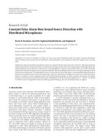
2.1. Data Model and Notation. A general fully connected
broadcasting sensor network with J nodes is considered, in
whicheachnodek has direct access to a specific set of M
k
microphones, with M =

J
k
=1
M
k
(see Figure 1). Nodes can
be either a hearing aid or a supporting external acoustic
sensor node. Each microphone signal m of node k can be
described in the frequency domain as
y
km
(
ω
)
= x
km
(

ω
)
+ v
km
(
ω
)
, m
= 1, , M
k
,
(1)
where x
km
(ω) is a desired speech component and v
km
(ω)an
undesired noise component. Although x
km
(ω)isreferredto
as the desired speech component, v
km
(ω) is not necessarily
nonspeech, that is, undesired speech sources may be included
in v
km
(ω). All subsequent algorithms will be implemented
in the frequency domain, where (1) is approximated based
on finite-length time-to-frequency domain transformations.
For conciseness, the frequency-domain variable ω will be

omitted. All signals y
km
of node k are stacked in an M
k
-
dimensional vector y
k
,andallvectorsy
k
are stacked in an
M-dimensional vector y. The vectors x
k
, v
k
and x, v are
similarly constructed. The network-wide data model can
now be written as y
= x + v. Notice that the desired
speech component x may consist of multiple desired source
signals, for example when a hearing aid user is listening to
a conversation between multiple speakers, possibly talking
simultaneously. If there are Q desired speech sources, then
x
= As,
(2)
where A is an M
× Q-dimensional steering matrix and s
a Q-dimensional vector containing the Q desired sources.
Matrix A contains the acoustic transfer functions (evaluated
at frequency ω) from each of the speech sources to all

microphones, incorporating room acoustics and micro-
phone characteristics.
2.2. Centralized Multichannel Wiener Filtering. The goal of
each node k is to estimate the desired speech component
x
km
in its mth microphone, selected to be the reference
microphone. Without loss of generality, it is assumed that
the reference microphone always corresponds to m
= 1. For
the time being, it is assumed that each node has access to all
microphone signals in the network. Node k then performs
a filter-and-sum operation on the microphone signals with
filter coefficients w
k
that minimize the following MSE cost
function:
J
k
(
w
k
)
= E




x
k1

−w
H
k
y



2

,(3)
where E
{·} denotes the expected value operator, and where
the superscript H denotes the conjugate transpose operator.
EURASIP Journal on Advances in Signal Processing 3
s
Q
A
.
.
.
.
.
.
.
.
.
.
.
.
.

.
.
x
11
x
1M
1
x
21
x
2M
2
x
J1
x
JM
J
v
11
v
1M
1
v
21
v
2M
2
v
J1
v

JM
1
y
11
y
1M
1
y
21
y
2M
2
y
J1
y
JM
J
M
1
y
1
Node 1
M
2
y
2
Node 2
M
J
y

J
Node J
M
y
.
.
.
.
.
.
.
.
.
Figure 1: Data model for a sensor network with J sensor nodes, in which node k collects M
k
noisy observations of the Q source signals in s.
Noticethatateachnodek, one such MSE problem is to
be solved for each frequency bin. The minimum of (3)
corresponds to the well-known Wiener filter solution:
w
k
= R
−1
yy
R
yx
e
k1
,
(4)

with R
yy
= E{yy
H
}, R
yx
= E{yx
H
},ande
k1
being an M-
dimensional vector with only one entry equal to 1 and all
other entries equal to 0, which selects the column of R
yx
corresponding to the reference microphone of node k. This
procedure is referred to as multi-channel Wiener filtering
(MWF). If the desired speech sources are uncorrelated to
the noise, then R
yx
= R
xx
= E{xx
H
}. In the remaining of
this paper, it is implicitly assumed that all Q desired sources
may be active at the same time, yielding a rank-Q speech
correlation matrix R
xx
.Inpractice,R
xx

is unknown, but can
be estimated from
R
xx
= R
yy
−R
vv
(5)
with R
vv
= E{vv
H
}. The noise correlation matrix R
vv
can
be (re-)estimated during noise-only periods and R
yy
can be
(re-)estimated during speech-and-noise periods, requiring a
voice activity detection (VAD) mechanism. Even when the
noise sources and the speech source are not stationary, these
practical estimators are found to yield good noise reduction
performance [15, 19].
3. Simulation Scenario and the Benefit of
External Acoustic Sensor Nodes
The performance of microphone array based noise reduction
typically increases with the number of microphones. How-
ever, the number of microphones that can be placed on a
hearing aid is limited, and the acoustic field is only sampled

locally, that is, at the hearing aid itself. Therefore, there is
often a large distance between the location of the desired
source and the microphone array, which results in signals
with low SNR. In fact, the SNR decreases with 6 dB for every
doubling of the distance between a source and a microphone.
The noise reduction performance can therefore be greatly
increased by using supporting external acoustic sensor nodes
that are connected to the hearing aid through a wireless
link.
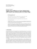
To assess the potential improvement that can be obtained
by adding external sensor nodes, a multi-source scenario is
simulated using the image method [21]. Figure 2 shows a
schematic illustration of the scenario. The room is cubical
(5 m
× 5m× 5 m) with a reflection coefficient of 0.4 at the
floor, the ceiling and at every wall. According to Sabine’s
formula this corresponds to a reverberation time of T
60
=
0.222 s. There are two hearing aid users listening to speaker
C, who produces a desired speech signal. One hearing aid
user has 2 hearing aids (node 2 and 3) and the other has one
hearing aid at the right ear (node 4). All hearing aids have
three omnidirectional microphones with a spacing of 1 cm.
Head shadow effects are not taken into account. Node 1 is
an external microphone array containing six omnidirectional
microphones placed 2 cm from each other. Speakers A and
B both produce speech signals interfering with speaker C.
All speech signals are sentences from the HINT (Hearing
in Noise Test) database [22]. The upper left loudspeaker

produces multi-talker babble noise (Auditec) with a power
normalized to obtain an input broadband SNR of 0 dB
in the first microphone of node 4, which is used as the
reference node. In addition to the localized noise sources, all
microphone signals have an uncorrelated noise component
which consist of white noise with power that is 10% of the
power of the desired signal in the first microphone of node
4. All nodes and all sound sources are in the same horizontal
plane, 2 m above ground level.
Notice that this is a difficult scenario, with many sources
and highly non-stationary (speech) noise. This kind of
scenario brings many practical issues, especially with respect
to reliable VAD decisions (cf. Section 7). Throughout this
paper, many of these practical aspects are disregarded. The
aim here is to demonstrate the benefit that can be achieved
4 EURASIP Journal on Advances in Signal Processing
5m
1m
Spacing: 2 cm
1.5m
2.5m
2m
5m
0.75 m
1.5m
0.5m
0.15 m
1m
2m
1

A
C
B2
3
4
Figure 2: The acoustic scenario used in the simulations throughout
this paper. Two persons with hearing aids are listening to speaker C.
The other sources produce interference noise.
with external sensor nodes, in particular in multi-source
scenarios. Furthermore, the theoretical performance of the
DANSE algorithm, introduced in Section 4, will be assessed
with respect to the centralized MWF algorithm. To isolate the
effects of VAD errors and estimation errors on the correlation
matrices, all experiments are performed in batch mode with
ideal VADs.
Two performance measures are used to assess the quality
of the noise reduction algorithms, namely the broadband
signal-to-noise ratio (SNR) and the signal-to-distortion ratio
(SDR). The SNR and SDR at node k are defined as
SNR
= 10 log
10
E


x
k
[
t
]

2

E


n
k
[
t
]
2

,(6)
SDR
= 10 log
10
E

x
k1
[
t
]
2

E

(
x
k1

[
t
]
− x
k
[
t
]
)
2

(7)
with
n
k
[t]andx
k
[t] the time domain noise component and
the desired speech component respectively at the output
at node k,andx
k1
[t] the desired time domain speech
component in the reference microphone of node k.
The sampling frequency is 32 kHz in all experiments. The
frequency domain noise reduction is based on DFT’s with
size equal to L
= 512 if not specified otherwise. Notice that L
is equivalent to the filter length of the time domain filters
that are implicitly applied to the microphone signals. The
DFT size L

= 512 is relatively large, which is due to the fact
that microphones are far apart from each other, leading to
higher time differences of arrival (TDOA) demanding longer
filters to exploit spatial information. If the filter lengths
are too short to allow a sufficient alignment between the
signals, then the noise reduction performance degrades. This
is evaluated in Section 6.4. To allow small DFT-sizes, yet large
distances between microphones, delay compensation should
be introduced in the local microphone signals or the received
signals at each node. However, since hearing aids typically
have hard constraints on the processing delay to maintain lip
synchronization, this delay compensation is restricted. This,
in effect, introduces a trade-off between input-output delay
and noise reduction performance.
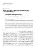
Figure 3(a) shows the output SNR and SDR of the
centralized MWF procedure at node 4 when five different
subsets of microphones are used for the noise reduction:
(1) the microphone signals of node 4 itself;
(2) the microphone signals of node 1 in addition to the
microphone signals of node 4 itself;
(3) the microphone signals of node 2 in addition to the
microphone signals of node 4 itself;
(4) the first microphone signal at every node in addition
to all microphone signals of node 4 itself; this is
equivalent to a scenario where the network support-
ing node 4 consists of single-microphone nodes, that
is, M
k
= 1, for k = 1, ,3;
(5) all microphone signals in the network.

The benefit of adding external microphones is very clear in
this graph. It also shows that microphones with a signifi-
cantly different position contribute more than microphones
that are closely spaced. Indeed, Cases 2, 3 and 4 both add
three extra microphone signals, but the benefit is largest in
Case 4, in which the additional microphones are relatively set
far apart. However, using multi-microphone nodes (Case 5)
still produces a significant benefit of about 25% (2 dB) in
comparison to single-microphone nodes (Case 4). Notice
that the benefit of placing external microphones, and the
benefit of using multi-microphone nodes in comparison to
single-microphone nodes, is of course very scenario specific.
For instance, if the vertical position of node 1 is reduced
by 0.5 m in Figure 2, then the difference between single-
microphone nodes (Case 4) and multi-microphone nodes
(Case 5) is more than 3 dB, as shown in Figure 3(b),which
correponds to an improvement of almost 50%.
4. The DANSE Algor i thm
In Section 3, simulations showed that adding external
microphones in addition to the microphones available in
a hearing aid may yield a great benefit in terms of both
noise suppression and speech distortion. Not surprisingly,
adding external nodes with multiple microphones boosts the
performance even more. However, the latter introduces a sig-
nificant increase in communication bandwidth, depending
on the number of microphones in each node. Furthermore,
the dimensions of the correlation matrix to be inverted in
formula (4) may grow significantly. However, if each node
has its own signal processor unit, this extra communication
bandwidth can be reduced and the computation can be

distributed by using the distributed adaptive node-specific
EURASIP Journal on Advances in Signal Processing 5
0
5
10
15
20
SDR (dB)
Node 4 + node 1 + node 2
+ single mic
of 1, 2, 3
All mics
Output SDR of MWF at node 4
0
2
4
6
8
10
12
SNR (dB)
Node 4 + node 1 + node 2
+ single mic
of 1, 2, 3
All mics
Output SNR of MWF at node 4
(a) Scenario of Figure 2
0
5
10

15
20
SDR (dB)
Node 4 + node 1 + node 2
+ single mic
of 1, 2, 3
All mics
Output SDR of MWF at node 4
0
2
4
6
8
10
SNR (dB)
Node 4 + node 1 + node 2
+ single mic
of 1, 2, 3
All mics
Output SNR of MWF at node 4
(b) Scenario of Figure 2 with vertical position of node 1 reduced by
0.5 m
Figure 3: Comparison of output SNR and SDR of MWF at node 4 for five different microphone subsets.
signal estimation (DANSE) algorithm, as proposed in [13,
14]. The DANSE algorithm computes the optimal network
wide Wiener filter in a distributed, iterative fashion. In this
section this algorithm is briefly reviewed and reformulated
in a noise reduction context.
4.1. The DANSE
K

Algorithm. In the DANSE
K
algorithm,
each node k estimates K different desired signals, corre-
sponding to the desired speech components in K of its
microphones (assuming that K
≤ M
k
, ∀ k ∈{1, , J}).
Without loss of generality, it is assumed that the first K
microphones are selected, that is, the signal to be estimated
is the K-channel signal
x
k
= [x
k1
···x
kK
]
T
. The first entry
in this vector corresponds to the reference microphone,
whereas the other K
−1 entries should be viewed as auxiliary
channels. They are required to fully capture the signal
subspace spanned by the desired source signals. Indeed, if K
is chosen equal to Q, the K channels of
x
k
define the same

signal subspace as defined by the channels in s, that is,
x
k
= A
k
s.
(8)
where A
k
denotes a K × K submatrix of the steering matrix
A in formula (2). K being equal to Q is a requirement for
DANSE
K
to be equivalent to the centralized MWF solution
(see Theorem 1). The case in which K
/
=Q is not considered
here. For a more detailed discussion why these auxiliary
channels are introduced, we refer to [13].
Each node k estimates its desired signal
x
k
with respect to
a corresponding MSE cost function
J
k
(
W
k
)

= E




x
k
−W
H
k
y



2

(9)
with W
k
an M × K matrix, defining a multiple-input
multiple-output (MIMO) filter. Notice that this corresponds
to K independent estimation problems in which the same M-
channel input signal y is used. Similarly to (3), the Wiener
solution of (9)isgivenby

W
k
= R
−1
yy

R
xx
E
k
(10)
with
E
k
=
⎡
⎣
I
K
O
(M−K)×K
⎤
⎦
(11)
with I
K
denoting the K × K identity matrix and O
U×V
denoting an all-zero U × V matrix. The matrix E
k
selects
the first K columns of R
xx
, corresponding to the K-channel
signal
x

k
. The DANSE
K
algorithm will compute (10)in
an iterative, distributed fashion. Notice that only the first
column of

W
k
is of actual interest, since this is the filter
that estimates the desired speech component in the reference
microphone. The auxiliary columns of

W
k
are by-products
of the DANSE
K
algorithm.
A partitioning of the matrix W
k
is defined as W
k
=
[W
T
k1
···W
T
kJ

]
T
where W
kq
denotes the M
k
×K submatrix of
W
k
that is applied to y
q
in (9). Since node k only has access
to y
k
, it can only apply the partial filter W
kk
.TheK-channel
output signal of this filter, defined by z
k
= W
H
kk
y
k
, is then
broadcast to the other nodes. Another node q can filter this
K-channel signal z
k
that it receives from node k by a MIMO
filter defined by the K

× K matrix G
qk
.Thisisillustratedin
6 EURASIP Journal on Advances in Signal Processing
y
1
y
2
y
3
M
1
M
2
M
3
W
11
W
22
W
33
K
K
K
z
1
z
2
z

3
G
12
G
13
G
21
G
23
G
31
G
32
x
1
x
2
x
3
Figure 4: The DANSE
K
scheme with 3 nodes (J = 3). Each
node k estimates the desired signal
x
k
using its own M
k
-channel
microphone signal, and 2 K-channel signals broadcast by the other
two nodes.

Figure 4 for a three-node network (J = 3). Notice that the
actual W
k
that is applied by node k is now parametrized as
W
k
=
⎡
⎢
⎢
⎢
⎢
⎢
⎢
⎢
⎣
W
11
G
k1
W
22
G
k2
.
.
.
W
JJ
G

kJ
⎤
⎥
⎥
⎥
⎥
⎥
⎥
⎥
⎦
. (12)
In what follows, the matrices G
kk
, ∀ k ∈{1, , J},are
assumed to be K
× K identity matrices I
K
to minimize the
degrees of freedom (they are omitted in Figure 4). Node k
can only manipulate the parameters W
kk
and G
k1
···G
kJ
.If
(8) holds, it is shown in [13] that the solution space defined
by the parametrization (12) contains the centralized solution

W

k
.
Noticethateachnodek broadcasts a K-channel (Here it
is assumed without loss of generality that K
≤ M
k
, ∀ k ∈
{
1, , J}; if this does not hold at a certain node k, this
node will transmit its unfiltered microphone signals) signal
z
k
, which is the output of the M
k
× K MIMO filter
W
kk
, acting both as a compressor and an estimator at the
same time. The subscript K thus refers to the (maximum)
number of channels of the broadcast signal. DANSE
K
compresses the data to be sent by node k by a factor of
max
{M
k
/K,1}. Further compression is possible, since the
channels of the broadcast signal z
k
are highly correlated,
but this is not taken into consideration throughout this

paper.
The DANSE
K
algorithm will iteratively update the ele-
ments at the righthand side of (12)tooptimallyestimate
the desired signals
x
k
, ∀ k ∈{1, , J}.Todescribe
this updating procedure, the following notation is used.
The matrix G
k
= [G
T
k1
···G
T
kJ
]
T
stacks all transformation
matrices of node k.ThematrixG
k,−q
defines the matrix G
k
in which G
kq
is omitted. The K(J − 1)-channel signal z
−k
is

defined as z
−k
= [z
T
1
···z
T
k
−1
z
T
k+1
···z
T
J
]
T
. In what follows,
asuperscripti refers to the value of the variable at iteration
step i. Using this notation, the DANSE
K
algorithm consists
of the following iteration steps:
(1) Initialize
i
← 0
k
← 1
∀ q ∈{1, , J}: W
qq

← W
0
qq
, G
q,−q
← G
0
q,
−q
, G
qq
←
I
K
,whereW
0
qq
and G
0
q,
−q
are random matrices of
appropriate dimension.
(2) Node k updates its local parameters W
kk
and G
k,−k
by solving a local estimation problem based on its
own local microphone signals y
k

together with the
compressed signals z
i
q
= W
iH
qq
y
q
thatitreceivesfrom
the other nodes q
/
=k, that is, it minimizes

J
i
k

W
kk
, G
k,−k

= E




x
k

−

W
H
kk
| G
H
k,
−k


y
i
k



2

, (13)
where
y
i
k
=

y
k
z
i

−k

.
(14)
Define
x
i
k
similarly as (14), but now only containing the
desired speech components in the considered signals. The
update performed by node k is then

W
i+1
kk
G
i+1
k,
−k

=


R
i
yy,k

−1

R

i
xx,k
E
k
(15)
with
E
k
=
⎡
⎣
I
K
O
(M
k
−K+K(J−1))×K
⎤
⎦
, (16)

R
i
yy,k
= E


y
i
k

y
iH
k

, (17)

R
i
xx,k
= E


x
i
k
x
iH
k

. (18)
The parameters of the other nodes do not change, that is,
∀ q ∈{1, , J}\{k} : W
i+1
qq
= W
i
qq
, G
i+1
q,

−q
= G
i
q,
−q
.
(19)
(3) W
kk
← W
i+1
kk
, G
k,−k
← G
i+1
k,
−k
k ← (k mod J)+1
i
← i +1
(4) Return to Step 2
Notice that node k updates its parameters W
kk
and G
k,−k
,
according to a local multi-channel Wiener filtering problem
with respect to its M
k

+(J − 1)K input channels.This MWF
EURASIP Journal on Advances in Signal Processing 7
problem is solved in the same way as the MWF problem given
in (3)or(9).
Theorem 1. Assume that K
= Q.Ifx
k
= A
k
s, ∀ k ∈
{
1, , J}, with A
k
afullrankK ×K matrix, then the DANSE
K
algorithm converges for any k to the optimal filters (10) for any
initialization of the parameters.
Proof. See [13].
Notice that DANSE
K
theoretically provides the same
output as the centralized MWF algorithm if K
= Q.The
requirement that
x
k
= A
k
s, ∀ k ∈{1, , J},issatisfied
because of (2). However, notice that the data model (2)is

only approximately fullfilled in practice due to a finite-length
DFT size. Consequently, the rank of the speech correlation
matrix R
xx
is not Q, but it has Q dominant eigenvalues
instead. Therefore, the theoretical claims of convergence and
optimality of DANSE
K
,withK = Q, are only approximately
true in practice due to frequency domain processing.
4.2. Simultaneous Updating. The DANSE
K
algorithm as
described in Section 4.1 performs sequential updating in a
round-robin fashion, that is, nodes update their parameters
one at a time. In [20], it is observed that convergence
of DANSE is no longer guaranteed when nodes update
simultaneously, or in an uncoordinated fashion where each
node decides independently in which iteration steps it
updates its parameters. This is however an interesting case,
since a simultaneous updating procedure allows for parallel
computation, and uncoordinated updating removes the need
for a network wide protocol that coordinates the updates
between nodes.
Let W
= [W
T
11
W
T

22
···W
T
JJ
]
T
, and let F(W) be the
function that defines the simultaneous DANSE
K
update of
all parameters in W, that is, F applies (15)
∀ k ∈{1, J}
simultaneously. Experiments in [20] show that the update
W
i+1
= F(W
i
) may lead to limit cycle behavior. To avoid
these limit cycles, the following relaxed version of DANSE is
suggested in [20]:
W
i+1
=

1 − α
i

W
i
+ α

i
F

W
i

(20)
with stepsizes α
i
satisfying
α
i
∈
(
0, 1
]
,
(21)
lim
i →∞
α
i
= 0, (22)
∞

i=0
α
i
=∞.
(23)

The suggested conditions on the stepsize α
i
are however
quite conservative and may result in slow convergence. In
most cases, the simultaneous update procedure converges
already when a constant value for α
i
is chosen ∀ i ∈ N
that is sufficiently small. In all simulations performed for the
scenario in Section 3,avalueofα
i
= 0.5, ∀ i ∈ N was found
to eliminate limit cycles in every setup.
5. Robust DANSE
5.1. Robustness Issues in DANSE. In Section 6, simulation
results will show that the DANSE algorithm does not achieve
the optimal noise reduction performance as predicted by
Theorem 1. There are two important reasons for this subop-
timal performance.
The first reason is the fact that the DANSE
K
algorithm
assumes that the signal space spanned by the channels of
x
k
is well-conditioned, ∀ k ∈{1, , J}. This assumption
is reflected in Theorem 1 by the condition that A
k
be full
rank for all k. Although this is mostly satisfied in practice,

the A
k
’s are often ill-conditioned. For instance, the distance
between microphones in a single node is mostly small,
yielding a steering matrix with several columns that are
almost identical, that is, an ill-conditioned matrix A
k
in the
formulation of Theorem 1.
The microphones of nodes that are close to a noise
source typically collect low SNR signals. Despite the low
SNR, these signals can boost the performance of the MWF
algorithm, since they can act as noise references to cancel
out noise in the signals recorded by other nodes. However,
the DANSE algorithm cannot fully exploit this since the
local estimation problem at such low SNR nodes is ill-
conditioned. If node k has low SNR microphone signals y
k
,
the correlation matrix
R
xx,k
= E{x
k
x
H
k
} has large estimation
errors, since the corresponding noise correlation matrix
R

vv,k
and the speech+noise correlation matrix R
yy,k
are very
similar, that is,
R
vv,k
≈ R
yy,k
. Notice that R
xx,k
is a submatrix
of

R
xx,k
defined in (18), which is used in the DANSE
K
algorithm. From another point of view, this also relates to
an ill-conditioned steering matrix A, since the submatrix A
k
is close to an all-zero matrix compared to the submatrices
corresponding to nodes with higher SNR signals.
5.2. Robust DANSE (R-DANSE). In this section, a modifica-
tion to the DANSE algorithm is proposed to achieve a better
noise reduction performance in the case of low SNR nodes or
ill-conditioned steering matrices. The main idea is to replace
an ill-conditioned A
k
matrix by a better conditioned matrix

by changing the estimation problem at node k. The new
algorithm is referred to as “robust DANSE” or R-DANSE.
In what follows, the notation v(p) is used to denote the p-
th entry in a vector v,andm(p) is used to denote the p-th
column in the matrix M.
For each node k, the channels in
x
k
that cause ill-
conditioned steering matrices, or that correspond to low
SNR signals, are discarded and replaced by the desired speech
components in the signal(s) z
i
q
received from other (high
SNR) nodes q
/
=k, that is,
x
i
k

p

=
w
i
qq
(
l

)
H
x
q
, q ∈{1, , J}\{k}, l ∈{1, ,K},
(24)
if x
kp
causes an ill-conditioned steering matrix or if x
kp
corresponds to a low SNR microphone, and
x
i
k

p

=
x
kp
(25)
8 EURASIP Journal on Advances in Signal Processing
otherwise. Notice that the desired signal
x
i
k
may now change
at every iteration, which is reflected by the superscript i
denoting the iteration index.
To decide whether to use (24)or(25), the condition

number of the matrix A
k
does not necessarily have to
be known. In principle, it is always better to replace the
K
− 1 auxiliary channels in x
k
as in formula (24), where
adifferent q should be chosen for every p. Indeed, since
microphones of different nodes are typically far apart from
each other, better conditioned steering matrices are then
obtained. Also, since the correlation matrix

R
xx,k
is better
estimated when high SNR signals are available, the chosen
q’s preferably correspond to high SNR nodes. Therefore,
the decision procedure requires knowledge of the SNR at
the different nodes. For a low SNR node k, one can also
replace all K channels in
x
k
as in (24), including the reference
microphone. In this case, there is no estimation of the speech
component that is collected by the microphones of node k
itself. However, since the network wide problem is now better
conditioned, the other nodes in the network will benefit from
this.
The R-DANSE

K
algorithm performs the same steps as
explained in Section 4.1 for the DANSE
K
algorithm, but now
x
i
k
replaces x
k
in (13)–(18). This means that in R-DANSE, the
E
k
matrix in (16) now may contain ones at row indices that
are higher than M
k
. To guarantee convergence of R-DANSE,
the placement of ones in (16), or equivalently the choices for
q and l in (24), is not completely free, as explained in the next
section.
5.3. Convergence of R-DANSE. To p r o v i d e c o n v e r g e n c e
results, the dependencies of each individual estimation
problem are described by means of a directed graph G with
KJ vertices, where each vertex corresponds to one of the
locally computed filters, that is, a specific column of W
kk
for
k
= 1 ···J. (Readers that are not familiar with the jargon
of graph theory might want to consult [23], although in

principle no prior knowledge on graph theory is assumed).
The graph contains an arc from filter a to b,describedby
the ordered pair (a,b), if the output of filter b contains the
desired speech component that is estimated by filter a.For
example, formula (24) defines the arc (w
kk
(p),w
qq
(l)). A
vertex v that has no departing arc is referred to as a direct
estimation filter (DEF), that is, the signal to be estimated
is the desired speech component in one of the node’s own
microphone signals, as in formula (25).
To illustrate this, a possible graph is shown in Figure 5
for DANSE
2
applied to the scenario described in Section 3,
where the hearing aid users are now listening to two speakers,
that is, speakers B and C. Since the microphone signals of
node 1 have a low SNR, the two desired signals in
x
1
that are
used in the computation of W
11
are replaced by the filtered
desired speech component in the received signals from
higher SNR nodes 2 and 4, that is, w
22
(1)

H
x
2
and w
44
(1)
H
x
4
,
respectively. This corresponds to the arcs (w
11
(1), w
22
(1))
and (w
11
(2), w
44
(1)). To calculate w
22
(1), w
33
(1), and w
44
(1),
the desired speech components x
21
, x
31

and x
41
in the
respective reference microphones are used. These filters
Node 1
w
11
(1)
w
11
(2)
Node 2
Node 3
Node 4
w
22
(1)
w
22
(2)
w
33
(1)
w
33
(2)
w
44
(1)
w

44
(2)
Figure 5: Possible graph describing dependencies of estimations
problems for DANSE
2
applied to the acoustic scenario described in
Section 3.
are DEF’s, and are shaded in Figure 5. The microphones at
node 2 are very close to each other. Therefore, to avoid an ill-
conditioned matrix A
2
at node 2, the signals to be estimated
by w
22
(2) should be provided by another node, and not by
another microphone signal of node 2 itself. Therefore, the
arc (w
22
(2), w
44
(1)) is added. For similar reasons, the arcs
(w
33
(2), w
44
(1)) and (w
44
(2), w
22
(1)) are also added.

Theorem 2. Let all assumptions of Theorem 1 be satisfied.
Let G be the directed graph describing the dependencies of the
estimation problems in the R-DANSE
K
algorithm as described
above. If G is acyclic, then the R-DANSE
K
algorithm converges
to the optimal filters to estimate the desired signals defined
by G.
Proof. The proof of Theorem 1 in [13] on convergence of
DANSE
K
is based on the assumption that the desired K-
channel signals
x
k
, ∀ k ∈{1, , J}, are all in the same K-
dimensional signal subspace spanned by the K sources in s,
that is,
x
k
= A
k
s.
(26)
This assumption remains valid in R-DANSE
K
. Indeed, since
x

q
contains M
q
linear combination of the Q sources in s, the
signal
x
i
k
(p)givenby(24) is again a linear combination of
the source signals. However, the coefficients of this linear
combinations may change at every iteration as the signal
x
i
k
(p) is an output of the adaptive filter w
i
qq
(l) in another
node q. This then leads to a modified version of Theorem 1
for DANSE
K
in which the matrix A
k
in (26)isnotfixed,but
may change at every iteration, that is,
x
i
k
= A
i

k
s.
(27)
EURASIP Journal on Advances in Signal Processing 9
Define
W
i
kq
= arg min
W
kq

min
G
k,−q
E




x
k
−

W
H
kq
| G
H
k,

−q


y
i
q



2


.
(28)
This corresponds to the hypothetical case in which node k
would optimise W
i
kq
directly, without the constraint W
i
kq
=
W
i
qq
G
i
kq
where node k depends on the parameter choice of
node q.

In [13]itisproventhatforDANSE
K
, under the
assumptions of Theorem 1, the following holds:
∀ q, k ∈{1, , J} :
W
i
kq
=
W
i
qq
A
kq
(29)
with A
kq
= A
−H
q
A
H
k
. This means that the columns of
W
i
qq
span a K-dimensional subspace that also contains the
columns of
W

i
kq
, which is the optimal update with respect
to the cost function J
i
k
of node k, as if there were no
constraints on W
i
kq
. Or in other words, an update by node q
automatically optimizes the cost function of any other node
k with respect to W
kq
,ifnodek performs a responding
optimization of G
kq
, yielding G
opt
kq
= A
kq
. Therefore, the
following expression holds:
∀ k ∈{1, , J},∀ i ∈ N :min
G
k,−k

J
i+1

k

W
i+1
kk
, G
k,−k

≤
min
G
k,−k

J
i
k

W
i
kk
, G
k,−k

.
(30)
Notice that this holds at every iteration for every node. In the
case of R-DANSE
K
, the A
kq

matrix of expression (29)changes
at every iteration. At first sight, expression (30) remains valid,
since changes in the matrix A
kq
are compensated by the
minimization over G
kq
in (30).However,thisisnottrue
since the desired signals
x
i
k
also change at every iteration, and
therefore the cost functions at different iterations cannot be
compared.
Expression (30) can be partitioned in K sub-expressions:
∀ p ∈{1, , K}, ∀ k ∈{1, , J}, ∀ i ∈ N :
(31)
min
g
k,−k
(p)

J
i+1
kp

w
i+1
kk


p

, g
k,−k

p


≤ min
g
k,−k
(p)

J
i
kp

w
i
kk

p

, g
k,−k

p



(32)
with

J
i
kp

w
kk
, g
k,−k

= E




x
k

p

−

w
H
kk
| g
H
k,

−k


y
i
k



2

. (33)
For the R-DANSE
K
case, (33) remains the same, except that
x
k
(p)hastobereplacedwithx
i
k
(p). As explained above,
due to this modification, expression (32) does not hold
anymore. However, it does hold for the cost functions J
i
kp
corresponding to a DEF w
kk
(p), that is, a filter for which
the desired signal is directly obtained from one of the
microphone signals of node k. Indeed, every DEF w

kk
(p)has
a well-defined cost function

J
i
kp
, since the signal x
i
k
(p)isfixed
over different iteration steps. Because

J
i
kp
has a lower bound,
(32) shows that the sequence
{min
g
p
k,
−k

J
i
kp
}
i∈N
converges. The

convergence of this sequence implies convergence of the
sequence
{w
i
kk
(p)}
i∈N
, as shown in [13].
After convergence of all w
kk
(p) parameters correspond-
ing to a DEF, all vertices in the graph G that are directly
connected to this DEF have a stable desired signal, and
their corresponding cost functions become well-defined. The
above argument shows that these filters then also converge.
Continuing this line of thought, convergence properties
of the DEF will diffuse through the graph. Since the graph
isacyclic,allverticesconverge.ConvergenceofallW
kk
parameters for k = 1 ···J automatically yields convergence
of all G
k
parameters, and therefore convergence of all W
k
filters for k = 1···J. Optimality of the resulting filters can
be proven using the same arguments as in the optimality
proof of Theorem 1 for DANSE
K
in [13].
6. Performance of DANSE and R-DANSE

In this section, the batch mode performance of DANSE and
R-DANSE is compared for the acoustic scenario of Section 3.
In this batch version of the algorithms, all iterations of
DANSE and R-DANSE are on the full signal length of about
20 seconds. In real-life applications, however, iterations
will of course be spread over time, that is, subsequent
iterations are performed on different signal segments. To
isolate the influence of VAD errors, an ideal VAD is used
in all experiments. Correlation matrices are estimated by
time averaging over the complete length of the signal. The
sampling frequency is 32 kHz and the DFT size is equal to
L
= 512 if not specified otherwise.
6.1. Experimental Validation of DANSE and R-DANSE. Three
different measures are used to assess the quality of the
outputs at the hearing aids: the signal-to-noise ratio (6),
the signal-to-distortion ratio (7), and the mean squared
error (MSE) between the coefficients of the centralized
multichannel Wiener filter
w
k
and the filter obtained by the
DANSE algorithm, that is,
MSE
=
1
L





w
k
−w
k
(1)


2
(34)
where the summation is performed over all DFT bins, with
L the DFT size,
w
k
defined by (4), and w
k
(1) denoting the
first column of W
k
in (12), that is, the filter that estimates
the speech component x
k1
in the reference microphone at
node k.
Two d ifferent scenarios are tested. In scenario 1 the
dimension Q of the desired signal space is Q
= 1, that is,
both hearing aid users are listening to speaker C, whereas
speakers A and B and the babble-noise loudspeaker are
considered to be background noise. In Figure 6, the three

quality measures are plotted (for node 4) versus the iteration
index for DANSE
1
and R-DANSE
1
, with either sequential
updating or simultaneous updating (without relaxation).
Also an upper bound is plotted, which corresponds to the
centralized MWF solution defined in (4). The R-DANSE
1
10 EURASIP Journal on Advances in Signal Processing
5
6
7
8
9
10
SNR (dB)
0 5 10 15 20 25 30
Iteration
Q
= 1: SNR of node 4 versus iteration
(a)
8
10
12
14
16
SDR (dB)
0 5 10 15 20 25 30

Iteration
Q
= 1: SDR of node 4 versus iteration
(b)
10
−5
10
−4
MSE
0 5 10 15 20 25 30
Iteration
Q = 1: MSE on filter coefficients of node 4 versus iteration
R-DANSE
1
sequential
R-DANSE
1
simultaneous
DANSE
1
sequential
DANSE
1
simultaneous
(c)
Figure 6: Scenario 1: SNR, SDR, and MSE on filter coefficients
versus iterations for DANSE
1
and R-DANSE
1

at node 4, for both
sequential and simultaneous updates. Speaker C is the only target
speaker.
graph consists of only DEF nodes, except for w
11
, which has
an arc (w
11
, w
44
) to avoid performance loss due to low SNR.
Since there is only one desired source, DANSE
1
theoretically
should converge to the upper bound performance, but this is
not the case. The R-DANSE
1
algorithm performs better than
the DANSE
1
algorithm, yielding an SNR increase of 1.5 to
2 dB, which is an increase of about 20% to 25%. The same
holds for the other two hearing aids, that is, node 2 and
3, which are not shown here. The parallel update typically
converges faster but it converges to a suboptimal limit cycle,
since no relaxation is used. Although this limit cycle is not
very clear in these plots, a loss in SNR of roughly 1 dB is
observed in every hearing aid. This can be avoided by using
relaxation, which will be illustrated in Section 6.2.
In scenario 2, the case in which Q

= 2isconsidered,
that is, there are two desired sources: both hearing aid users
are listening to speakers B and C, who talk simultaneously,
yielding a speech correlation matrix R
xx
of approximately
rank 2. The R-DANSE
2
graph is illustrated in Figure 5.
For this 2-speaker case, both DANSE
1
and DANSE
2
are
evaluated, where the latter should theoretically converge to
the upper bound performance. The results for node 4 are
plotted in Figure 7. While the MSE is lower for DANSE
2
compared to DANSE
1
, it is observed that DANSE
2
does not
reach the optimal noise reduction performance. R-DANSE
2
6
8
10
12
SNR (dB)

0 5 10 15 20 25 30
Iteration
Q
= 2: SNR of node 4 versus iteration
(a)
12
14
16
SDR (dB)
0 5 10 15 20 25 30
Iteration
Q
= 2: SDR of node 4 versus iteration
(b)
10
−5
10
−4
MSE
0 5 10 15 20 25 30
Iteration
Q = 2: MSE on filter coefficients of node 4 versus iteration
R-DANSE
2
R-DANSE
1
DANSE
2
DANSE
1

(c)
Figure 7: Scenario 2: SNR, SDR and MSE on filter coefficients
versus iterations for DANSE
1
, R-DANSE
1
,DANSE
2
and R-DANSE
2
at node 4. Speakers B and C are target speakers.
is however able to reach the upper bound performance at
every hearing aid. The SNR improvement of R-DANSE
2
in comparison with DANSE
2
is between 2 and 3 dB at
every hearing aid, which is again an increase of about 20%
to 25%. Notice that R-DANSE
2
even slightly outperforms
the centralized algorithm. This may be because R-DANSE
2
performs its matrix inversions on correlation matrices with
smaller dimensions than the all-microphone correlation
matrix R
yy
in the centralized algorithm, which is more
favorable in a numerical sense.
6.2. Simultaneous Updating with Relaxation. Simulations

on different acoustic scenarios show that in most cases,
DANSE
K
with simultaneous updating results in a limit
cycle oscillation. The occurrence of limit cycles appears to
depend on the position of the nodes and sound sources, the
reverberation time, as well as on the DFT size, but no clear
rule was found to predict the occurrence of a limit cycle.
To illustrate the effect of relaxation, the simulation results
of R-DANSE
1
in the scenario of Section 3 are given in
Figure 8(a), where now the DFT size is L
= 1024, which
results in clearly visible limit cycle oscillations when no
relaxation is used. This causes an over-all loss in SNR of 2
or 3 dB at every hearing aid.
Figure 8(b) shows the same experiment where relaxation
is used as in formula (20)withα
i
= 0.5, ∀ i ∈ N.
EURASIP Journal on Advances in Signal Processing 11
5
10
15
20
SDR (dB)
0 5 10 15 20 25 30
Iteration
Q

= 1: SDR of node 4 versus iteration
0
5
10
15
SNR (dB)
0 5 10 15 20 25 30
Iteration
Q
= 1: SNR of node 4 versus iteration
R-DANSE
1
sequential
R-DANSE
1
simultaneous
(a) without relaxation
5
10
15
20
SDR (dB)
0 5 10 15 20 25 30
Iteration
Q
= 1: SDR of node 4 versus iteration
0
5
10
15

SNR (dB)
0 5 10 15 20 25 30
Iteration
Q
= 1: SNR of node 4 versus iteration
R-DANSE
1
sequential
R-DANSE
1
simultaneous
(b) with relaxation (α
i
= 0.5, ∀ i ∈ N)
Figure 8: SNR and SDR for R-DANSE
1
versus iterations at node 4 with sequential and simultaneous updating.
In this case, the limit cycle does not appear and the simul-
taneous updating algorithm indeed converges to the same
values as the sequential updating algorithm. Notice that the
simultaneous updating algorithm converges faster than the
sequential updating algorithm.
6.3. DFT Size. In Figure 9, the SNR and SDR of the output
signal of R-DANSE
1
at nodes 3 and 4 is plotted as a function
of the DFT size L, which is equivalent to the length of the
time domain filters that are implicitly applied to the signals
at the nodes. 28 iterations were performed with sequential
updating for L

= 256, L = 512, L = 1024, and L = 2048. The
outputs of the centralized version and the scenario in which
nodes do not share any signals, are also given as a reference.
As expected, the performance increases with increasing
DFT size. However, the discrepancy between the centralized
algorithm and R-DANSE
1
grows for increasing DFT size.
One reason for this observation is that, for large DFT sizes,
R-DANSE often converges slowly once the filters at all nodes
are close to the optimal filters.
The scenario with isolated nodes is less sensitive to the
DFT size. This is because the tested DFT sizes are quite large,
yielding long filters. As explained in the next section, shorter
filter lengths are sufficient in the case of isolated nodes since
the microphones are very close to each other, yielding small
time differences of arrival (TDOA).
6.4. Communication Delays or Time Differences of Ar rival. To
exploit the spatial coherence between microphone signals,
the noise reduction filters attempt to align the signal compo-
nents resulting from the same source in the different micro-
phone signals. However, alignment of the direct components
of the source signals is only possible when the filter lengths
are at least twice the maximum time difference of arrival
(TDOA) between all the microphones. This means that
in general, the noise reduction performance degrades with
increasing TDOA’s and fixed filter lengths. Large TDOA’s
require longer filters, or appropriate delay compensation.
As already mentioned in Section 3,delaycompensation
is restricted in hearing aids due to lip synchronization

constraints.
The TDOA depends on the distance between the
microphones, the position of the sources and the delay
introduced by the communication link. Figure 10 shows
the performance degradation of R-DANSE at nodes 3 and
4 when the TDOA increases, in this case modelled by an
increasing communication delay between the nodes. There
is no delay compensation, that is, none of the signals are
delayed before filtering. DFT sizes L
= 512 and L = 1024 are
evaluated. The outputs of the centralized MWF procedure
are also given as a reference, as well as the procedure where
every node broadcasts its first microphone signal, which
corresponds to the scenario in which all supporting nodes
are single-microphone nodes. The lower bound is defined
by the scenario where all nodes are isolated, that is, each
node only uses its own microphones in the estimation
process.
As expected, when the communication delay increases,
the performance degrades due to increasing time lags
between signals. At node 3, the R-DANSE algorithm is
slightly more sensitive to the communication delay than the
centralized MWF. The behavior at node 2 is very similar,
and is omitted here. Furthermore, for large communication
delays, R-DANSE is outperformed by the single-microphone
nodes scenario. At node 4, both the centralized MWF and
12 EURASIP Journal on Advances in Signal Processing
2
4
6

8
10
12
14
16
SDR (dB)
200 400 600 800 1000 1200 1400 1600 1800 2000 2200
DFT size
Q
= 1: SDR of node 3 versus DFT size
−5
0
5
10
15
SNR (dB)
200 400 600 800 1000 1200 1400 1600 1800 2000 2200
DFT size
Q
= 1: SNR of node 3 versus DFT size
R-DANSE
1
Optimal
Isolated
(a) node 3
6
8
10
12
14

16
18
20
SDR (dB)
200 400 600 800 1000 1200 1400 1600 1800 2000 2200
DFT size
Q
= 1: SDR of node 4 versus DFT size
0
2
4
6
8
10
12
14
16
SNR (dB)
200 400 600 800 1000 1200 1400 1600 1800 2000 2200
DFT size
Q
= 1: SNR of node 4 versus DFT size
R-DANSE
1
Optimal
Isolated
(b) node 4
Figure 9: Output SNR and SDR after 28 iterations of R-DANSE
1
with sequential updating versus DFT size L at nodes 3 and 4.

2
4
6
8
10
12
14
16
SDR (dB)
0 100 200 300 400 500 600 700 800 900
Number of samples communication delay
Q
= 1: SDR of node 3 versus communication delay
−4
−2
0
2
4
6
8
10
12
14
SNR (dB)
R-DANSE L = 512
Centralized L
= 512
One mic of other nodes L
= 512
Isolated L

= 512
R-DANSE L
= 1024
Centralized L
= 1024
One mic of other nodes L
= 1024
Isolated L
= 1024
0 100 200 300 400 500 600 700 800 900
Number of samples communication delay
Q
= 1: SNR of node 3 versus communication delay
(a) node 3
6
8
10
12
14
16
18
20
SDR (dB)
0 100 200 300 400 500 600 700 800 900
Number of samples communication delay
Q
= 1: SDR of node 4 versus communication delay
2
4
6

8
10
12
14
SNR (dB)
R-DANSE L = 512
Centralized L
= 512
One mic of other nodes L
= 512
Isolated L
= 512
R-DANSE L
= 1024
Centralized L
= 1024
One mic of other nodes L
= 1024
Isolated L
= 1024
0 100 200 300 400 500 600 700 800 900
Number of samples communication delay
Q
= 1: SNR of node 4 versus communication delay
(b) node 4
Figure 10: Output SNR and SDR at nodes 3 and 4 after 12 iterations of R-DANSE
1
with sequential updating vs. delay of the communication
link.
EURASIP Journal on Advances in Signal Processing 13

the single-microphone nodes scenario even benefit from
communication delays. Apparently, the additional delay
allows the estimation process to align the signals more
effectively.
ThereasonwhyR-DANSEismoresensitivetoacom-
munication delay than the centralized MWF is that the latter
involves independent estimation processes, whereas in R-
DANSE, the estimation at any node k depends on the quality
of estimation at every other node q
/
=k.Noticehowever
that the influence of communication delay is of course very
dependent on the scenario and its resulting TDOA’s. The
above results only give an indication of this influence.
7. Practical Issues and Open Problems
In the batch-mode simulations provided in this paper, some
practical aspects have been disregarded. Therefore, the actual
performance of the MWF and the DANSE
K
algorithm may
be worse than what is shown in the simulations. In this
section, some of these practical aspects are briefly discussed.
The VAD is a crucial ingredient in MWF-based noise
reduction applications. A simple VAD may not behave well in
the simulated scenario as described in Figure 2 due to the fact
that the noise component also contains competing speech
signals. Especially the VADs at nodes that are close to an
interfering speech source (e.g., node 1 in Figure 2)arebound
to make many wrong decisions, which will then severely
deteriorate the output of the DANSE algorithm. To solve this,

a speaker selective VAD should be used, for example, [24].
Also, low SNR nodes should be able to use VAD information
from high SNR nodes. By sharing VAD information, better
VAD decisions can be made [25]. How to organize this, and
how a consensus decision can be found between different
nodes, is still an open research problem.
A related problem is the actual selection of the desired
source, versus the noise sources. A possible strategy is that
the speech source with the highest power at a certain
reference node is selected as the desired source. In hearing aid
applications, it is often assumed that the desired source is in
front of the listener. Since the actual positions of the hearing
aid microphones are known (to a certain accuracy), the VAD
can be combined with a source localization algorithm or a
fixed beamformer to distinguish between a target speaker
and an interfering speaker. Again, this information should be
shared between nodes so that all nodes can eventually make
consistent selections.
A practical aspect that needs special attention is the
adaptive estimation of the correlation matrices in the
DANSE
K
algorithm. In many MWF implementations, cor-
relation matrices are updated with the instantaneous sample
correlation matrix and by using a forgetting factor 0 <λ<1,
that is,
R
yy
[
t

]
= λR
yy
[
t
−1
]
+
(
1 − λ
)
y
[
t
]
y
H
[
t
]
,
(35)
where y[t] denotes the sample of the multi-channel signal
y at time t. The forgetting factor λ is chosen close to 1 to
obtain long-term estimates that mainly capture the spatial
coherence between the microphone signals. In the DANSE
K
algorithm, however, the statistics of the input signal y
k
in

node k,definedby(14), change whenever a node q
/
=k
updates its filters, since some of the channels in
y
k
are indeed
outputs from a filter in node q. Therefore, when node q
updates its filters, parts of the estimated correlation matrices

R
yy,k
and

R
xx,k
, ∀ k ∈{1, , J}\{q}, may become invalid.
Therefore, strategy (35) may not work well, since every new
estimate of the correlation matrix then relies on previous
estimates. Instead, either downdating strategies should be
considered, or the correlation matrices have to be completely
recomputed.
8. Conclusions
The simulation results described in this paper demonstrate
that noise reduction performance in hearing aids may be sig-
nificantly improved when external acoustic sensor nodes are
added to the estimation process. Moreover, these simulation
results provide a proof-of-concept for applying DANSE
K
in

cooperative acoustic sensor networks for distributed noise
reduction applications, such as in hearing aids. A more
robust version of DANSE
K
, referred to as R-DANSE
K
,has
been introduced and convergence has been proven. Batch-
mode experiments showed that R-DANSE
K
significantly
outperforms DANSE
K
. The occurrence of limit cycles and
the effectiveness of relaxation in the simultaneous updating
procedure has been illustrated. Additional tests have been
performed to quantify the influence of several parameters,
such as the DFT size and TDOA’s or delays within the
communication link.
Acknowledgments
This research work was carried out at the ESAT lab-
oratory of Katholieke Universiteit Leuven, in the frame
of the Belgian Programme on Interuniversity Attraction
Poles, initiated by the Belgian Federal Science Policy Office
IUAP P6/04 (DYSCO, “Dynamical systems, control and
optimization”, 2007–2011), the Concerted Research Action
GOA-AMBioRICS, and Research Project FWO no. G.0600.08
(“Signal processing and network design for wireless acoustic
sensor networks”). The scientific responsibility is assumed by
its authors. The authors would like to thank the anonymous

reviewers for their helpful comments.
References
[1] H. Dillon, Hearing Aids, Boomerang Press, Turramurra,
Australia, 2001.
[2] B. Kollmeier, J. Peissig, and V. Hohmann, “Real-time multi-
band dynamic compression and noise reduction for binaural
hearing aids,” Journal of Rehabilitation Research and Develop-
ment, vol. 30, no. 1, pp. 82–94, 1993.
[3] J. G. Desloge, W. M. Rabinowitz, and P. M. Zurek,
“Microphone-array hearing aids with binaural output . I.
Fixed-processing systems,” IEEE Transactions on Speech and
Audio Processing, vol. 5, no. 6, pp. 529–542, 1997.
[4] D. P. Welker, J. E. Greenberg, J. G. Desloge, and P. M. Zurek,
“Microphone-array hearing aids with binaural output. II.
14 EURASIP Journal on Advances in Signal Processing
A two-microphone adaptive system,” IEEE Transactions on
Speech and Audio Processing, vol. 5, no. 6, pp. 543–551, 1997.
[5] I.L.D.M.Merks,M.M.Boone,andA.J.Berkhout,“Design
of a broadside array for a binaural hearing aid,” in Proceedings
of IEEE Workshop on Applications of Signal Processing to Audio
and Acoustics (WASPAA ’97), October 1997.
[6] V. Hamacher, “Comparison of advanced monaural and
binaural noise reduction algorithms for hearing AIDS,” in
Proceedings of IEEE International Conference on Acoustics,
Speech and Signal Processing (ICASSP ’02), vol. 4, pp. 4008–
4011, May 2002.
[7] R. Nishimura, Y. Suzuki, and F. Asano, “A new adaptive bin-
aural microphone array system using a weighted least squares
algorithm,” in Proceedings of IEEE International Conference on
Acoustics, Speech and Signal Processing (ICASSP ’02), vol. 2, pp.

1925–1928, May 2002.
[8] T.WittkopandV.Hohmann,“Strategy-selectivenoisereduc-
tion for binaural digital hearing aids,” Speech Communication,
vol. 39, no. 1-2, pp. 111–138, 2003.
[9] M.E.Lockwood,D.L.Jones,R.C.Bilger,etal.,“Performance
of time- and frequency-domain binaural beamformers based
on recorded signals from real rooms,” The Journal of the
Acoustical Society of America, vol. 115, no. 1, pp. 379–391,
2004.
[10] T. Lotter and P. Vary, “Dual-channel speech enhancement by
superdirective beamforming,” EURASIP Journal on Applied
Signal Processing, vol. 2006, Article ID 63297, 14 pages, 2006.
[11] O. Roy and M. Vetterli, “Rate-constrained beamforming for
collaborating hearing aids,” in Proceedings of IEEE Interna-
tional Symposium on Information Theory (ISIT ’06), pp. 2809–
2813, July 2006.
[12] S. Doclo and M. Moonen, “GSVD-based optimal filtering
for single and multimicrophone speech enhancement,” IEEE
Transactions on Signal Processing, vol. 50, no. 9, pp. 2230–2244,
2002.
[13] A. Bertrand and M. Moonen, “Distributed adaptive node-
specific signal estimation in fully connected sensor
networks—Part I: sequential node updating,” Internal Report,
Katholieke Universiteit Leuven, ESAT/SCD, Leuven-Heverlee,
Belgium, 2009.
[14] A. Bertrand and M. Moonen, “Distributed adaptive estima-
tion of correlated node-specific signals in a fully connected
sensor network,” in Proceedings of IEEE International Confer-
ence on Acoustics, Speech and Signal Processing (ICASSP ’09),
pp. 2053–2056, April 2009.

[15] T.J.Klasen,T.VandenBogaert,M.Moonen,andJ.Wouters,
“Binaural noise reduction algorithms for hearing aids that
preserve interaural time delay cues,” IEEE Transactions on
Signal Processing, vol. 55, no. 4, pp. 1579–1585, 2007.
[16] S. Doclo, R. Dong, T. J. Klasen, J. Wouters, S. Haykin, and M.
Moonen, “Extension of the multi-channel wiener filter with
ITD cues for noise reduction in binaural hearing aids,” in
Proceedings of the International Workshop on Acoustic Echo and
Noise Control (IWAENC ’05), pp. 221–224, September 2005.
[17] S.Doclo,T.J.Klasen,T.VandenBogaert,J.Wouters,andM.
Moonen, “Theoretical analysis of binaural cue preservation
using multi-channel Wiener filtering and interaural transfer
functions,” in Proceedings of the International Workshop on
Acoustic Echo and Noise Control (IWAENC ’06),September
2006.
[18] T. Van den Bogaert, J. Wouters, S. Doclo, and M. Moonen,
“Binaural cue preservation for hearing aids using an interaural
transfer function multichannel wiener filter,” in Proceedings of
IEEE International Conference on Acoustics, Speech and Signal
Processing (ICASSP ’07), vol. 4, pp. 565–568, April 2007.
[19]S.Doclo,M.Moonen,T.VandenBogaert,andJ.Wouters,
“Reduced-bandwidth and distributed MWF-based noise
reduction algorithms for binaural hearing aids,” IEEE Trans-
actions on Audio, Speech, and Language Processing, vol. 17, no.
1, pp. 38–51, 2009.
[20] A. Bertrand and M. Moonen, “Distributed adaptive
node-specific signal estimation in fully connected sensor
networks—Part II: simultaneous & asynchronous node
updating,” Internal Report, Katholieke Universiteit Leuven,
ESAT/SCD, Leuven-Heverlee, Belgium, 2009.

[21] J. B. Allen and D. A. Berkley, “Image method for efficiently
simulating small-room acoustics,” The Journal of the Acoustical
Society of America, vol. 65, no. 4, pp. 943–950, 1979.
[22] M. Nilsson, S. D. Soli, and J. A. Sullivan, “Development of the
hearing in noise test for the measurement of speech reception
thresholds in quiet and in noise,” TheJournaloftheAcoustical
Society of America, vol. 95, no. 2, pp. 1085–1099, 1994.
[23] J. A. Bondy and U. S. R. Murty, Graph Theory with Applica-
tions, American Elsevier, New York, NY, USA.
[24] S. Maraboina, D. Kolossa, P. K. Bora, and R. Orglmeis-
ter, “Multi-speaker voice activity detection using ICA and
beampattern analysis,” in Proceedings of the European Signal
Processing Conference (EUSIPCO ’06), 2006.
[25] V. Berisha, H. Kwon, and A. Spanias, “Real-time implemen-
tation of a distributed voice activity detector,” in Proceedings
of IEEE Sensor Array and Multichannel Signal Processing
Workshop (SAM ’06), pp. 659–662, July 2006.