Study on the propagation of inlet flow distortion in axial compressor using an integral method_1 ppt
Bạn đang xem bản rút gọn của tài liệu. Xem và tải ngay bản đầy đủ của tài liệu tại đây (291.93 KB, 10 trang )
Chapter 1
Study on the Propagation of Inlet Flow Distortion
in Axial Compressor Using an Integral Method
An integral method is presented in this chapter. The integral method is proposed by
Kim et al. at 1996 aimed to describe the problems of distorted inlet flow propagation
in axial compressors. In this method, the detained blade rows are replaced by their
equivalent force field, and the Navier-Stokes equation can be simplified by using in-
tegral technique. Despite the great simplifications adopted in the integral method,
the multistage axial compressor with large inlet distortion, including back flow can
be analyzed and a qualitative trend of distortion propagation can be described
successfully. The integral method provides the useful information about the per-
formance of the axial compressor with inlet distortion, which is meaningful to engi-
neering application in the design and analysis of turbomachinery.
In this chapter, by applying the integral method, the effects of the parameters of
inlet distortions on the trend of downstream flow feature in compressor calculated
numerically is described. Other than the ratio of drag-to-lift coefficients of the
blade and the angle of flow, the value of distorted inlet velocity is found to be
another essential parameter to control the distortion propagation. Based on this
calculation, a critical distortion line and corresponding distortion propagation fac-
tor are proposed to express the effect of the two main inlet parameters: the angle
of flow and the distorted inlet velocity, on the propagation of distortion. From
the viewpoint of compressor efficiency, the distortion propagation is further de-
scribed by a compressor critical performance. The results present a useful physical
insight of compressor axial behavior and asymptotic behavior of the propagation
of inlet distortion, and confirm the active role of compressor in determining the
velocity distribution when compressor responds to an inlet flow distortion.
1.1 Introduction
In the operation of aircraft jet-engine, it is important to understand the aerody-
namic response resulting from an inlet flow distortion. An inlet flow distortion
may cause the rotating stall or even surge, or a combination of them. If the blades
fail to produce required loading, catastrophic damage to the complete engine
would result. To avoid stall and surge of compressor due to flow distortion, and
2
understand further, the inlet distortion and its propagation effects have received
much attention over the years. In 1955, Harry and Lubick [7] investigated the tur-
bojet engine in an altitude chamber at the NACA Lewis laboratory to determine
the effects of a wide range of uneven inlet-air pressure distributions on transient
characteristics and stall phenomenon.
The flow non-uniformities due to inlet distortion are commonly grouped into
radially varying steady state, circumferentially varying steady state and unsteady
distortions [5]. In many situations, the principal loss in stall margin can be regarded
as due to one of the above three groups. Among them, the flow with circumferential
distortion introduces new phenomenon into the fluid dynamic analysis of the com-
pressor behavior and has gained much attention by many researchers. One of the
methods used is a linearized approach, which provides quantitative information
about the performance of the compressor in a circumferentially non-uniform flow.
Several models, such as the parallel compressor model and its extensions, are used
to assess the compressor stability with inlet distortion. The numerical solution of the
time dependent nonlinear inviscid equations of motion is another method to study
the problem of compressor stability in a distorted flow.
In 1980, Stenning [11] presented some simpler techniques for analyzing the ef-
fects of circumferential inlet distortion. Stenning concluded that it is impossible to
achieve a complete success in calculating the distorted performance and distortion
attenuation of an axial compressor even though the use of high speed computers
has greatly improved the accuracy of performance analysis somewhat. However,
as an attempt, it is necessary to study the distorted performance and distortion at-
tenuation of an axial compressor even though a complete success may not be
achievable. As a first approach, the methods that use the known undistorted per-
formance characteristic as a starting point to predict the behavior of the compres-
sor with distortion are developed with a much prospect for success. A number of
investigators ([2], [3], [5], [6], [10]) have developed models for response to circum-
ferential distortion which use the undistorted compressor performance or stage
characteristics to predict the behavior with distortion. One novel real time correla-
tion scheme for the detection of operations (both steady state and transient) near to
the stability boundary of a compressor has recently been studied at the Georgia In-
stitute of Technology [9]. The information provided by the correlation scheme is
stochastic in nature to facilitate controller design [4]. The scheme has been
linked to the engine fuel controller and was used detect and avoid impending stall
by modulating the transient fuel schedule during operability tests [1].
Kim et al. [8] also successfully calculated the qualitative trend of distorted per-
formance and distortion attenuation of an axial compressor by using a simple inte-
gral method. This simple integral method was applied to describe the qualitative
trend of distortion propagation in axial compressors. Kim et al. concluded that the
two key parameters to control the distortion propagation are the ratio of drag-to-
lift coefficients of the blade and the angle of flow. The integral method pro-
vides the useful physical insight and qualitative information about the perform-
ance of the axial compressor with inlet distortion. It is meaningful to make use of
and develop this method further.
Chapter 1 Study on the Propagation of Inlet Flow Distortion
3
In this chapter, the integral method is confirmed and further improved. An in-
vestigation is progressed to understand the downstream flow feature with the inlet
distortion, including the velocity and mass flow rate. A critical distortion line is
presented to express the effect of two essential inlet parameters on the propagation
of distortion. The critical distortion line is simple, efficient and complete expres-
sion to analyze the propagation of inlet distortion in axial compressor. Finally, the
compressor critical performance and critical characteristic are also discussed.
1.2 Theoretical Formulation
Consider a two-dimensional inviscid flow through an axial compressor as shown
in [8]. The computational domain is shown in Fig. 1.1. The flow is described by
equations of continuity and motion:
0=
∂
∂
+
∂
∂
y
v
x
u
(1.1)
x
F
p
x
uv
y
u
x
=
∂
∂
+
∂
∂
+
∂
∂
)()()(
2
ρ
(1.2)
y
F
p
y
v
y
uv
x
=
∂
∂
+
∂
∂
+
∂
∂
)()()(
2
ρ
(1.3)
distorted
inlet
undistorted
inlet
v, y
u, x
δ
δ
(Y (x)
y=Y (x)+2 R
2
1
+Y (x))
1
π
y=Y(x)
=1/2
y=Y (x)
2
y=Y (x)
1
2R
π
distorted
inlet
undistorted
inlet
v,
u, x
1
1
2R
π
η=1
2R
π
η=−1
η=0
η= /δ−1
/δ
η
coordinates transfer from (x, y) to (x,η) :
Fig. 1.1. A schematic of coordinates transfer of calculation domain
1.2 Theoretical Formulation
The coordinate system is transferred from (x, y) to (x,
η
) by:
δ
η
)x(Yy −
=
(1.4)
here )x(Yy = is a symmetric line of distorted region, and
δ
is a half height of
distorted region.
If the static pressure takes circumferentially uniform, then:
)x(
pp
ρρ
≡
(1.5)
Before integrating the x- and y- momentum equations, and mass conservation
equation in distorted region, undistorted region and overall region, respectively, some
assumptions and parameters definitions are given for velocity, pressure and forces.
1.2.1 Velocity and Pressure
Assume the inlet velocity has a windward angle of
0
θ
, then
000
tan V U
γ
θ
==
(1.6)
where
0
U
and
0
V
are the x- and y- components of inlet velocity, respectively.
α
and
β
are the x- and y-velocity increments in the distorted inlet region, and
0
α
and
0
β
are the x- and y-velocity increments in the undistorted inlet region,
respectively.
In distorted region:
0
Uu
α
=
(1.7)
0
Vv
β
=
(1.8)
In undistorted region:
00
Uu
α
=
(1.9)
00
Vv
β
=
(1.10)
Chapter 1 Study on the Propagation of Inlet Flow Distortion 4
2
0
)V2(21
p
P
ρ
=
(1.11)
The non-dimensionalized velocity parameter (rotor speed) is
0
V2R
=
ω
. The
pressure is non-dimensionalized by
2
0
)V2(
2
1
ρ
:
1.2.2 Forces
(
)( )
*22
L
S
tantanvu
2
1
kF
θθ
−+=
⊥
(1.12)
(
)( )
2
*22
D
S
II
tantanvu
2
1
kF
θθ
−+=
(1.13)
()
[
]
()
*
2
2
L
R
tantanvRu
2
1
kF
ψψω
−−+=
⊥
(1.14)
()
[
]
()
2
*
2
2
D
R
II
tantanvRu
2
1
kF
ψψω
−−+=
(1.15)
The force components for a unit circumferential distance of the entire blade row are:
()
(
)
θθ
λ
λ
ψψ
λ
λ
cosFsinFcosFsinFF
S
II
S
S
R
II
R
R
x
−+−=
⊥⊥
(1.16)
()
(
)
θθ
λ
λ
ψψ
λ
λ
sinFcosFsinFcosFF
S
II
S
S
R
II
R
R
y
−−++=
⊥⊥
(1.17)
1.2 Theoretical Formulation 5
As shown in Fig. 1.2, in integral equations,
x
F
and
y
F
denote the forces in the dis-
torted inlet region, and
0,x
F
and
0,y
F
denote the forces in the undistorted inlet region,
respectively.
F
θ
v
u
F
⊥
F
//
F
⊥
F
⊥
⊥
F
//
F
//
F
//
λ
s
λ
r
R
OT O
R
ST
A
TO
R
θ
r
s
u
ω
R
-v
Fig. 1.2. The force diagram and velocities in the compressor stage
{ ()
[
]
()
()
[
]
(
)
}
{
()( ) ()( )
}
θθθθθθ
λ
λ
ψψψωψψψω
λ
λ
costantanvu
2
k
sintantanvu
2
k
costantanvRu
2
k
sintantanvRu
2
k
F
2
*22
D
*22
L
S
2
*
2
2
D
*
2
2
LR
x
−+−−++
−−+−−−+=
()
[
]
[ ]
2
22 2 *
RL
00
*2
D
222
L
22 22 * *2
S
LD
00
222
L
k22
U2 V( tan)
2
k2
( tan )
k
(2 )
kk
(U V)( tan ) ( tan )
2k
λββ
αβ γψγ
λαα
βα
γψ
α
αβγ
λ
βββ α
αβ γθγ γθ
λααα
α
βγ
−−
⎡⎤
=+− −
⎣⎦
−
−−
+−
++−−−
+
(1.20)
{ ()
[
]
()
()
[
]
(
)
}
{
()( ) ()( )
}
θθθθθθ
λ
λ
ψψψωψψψω
λ
λ
sintantanvu
2
k
costantanvu
2
k
sintantanvRu
2
k
costantanvRu
2
k
F
2
*22
D
*22
L
S
2
*
2
2
D
*
2
2
LR
y
−+−−+−+
−−++−−+=
()
[
]
[ ]
2
22 2 *
RL
00
*2
D
222
L
22 22 * *2
S
LD
00
222
L
k2
U2 V( tan)
2
k2 2
( tan )
k
(2 )
kk
(U V)( tan ) ( tan )
2k
λβ
αβ γψ
λα
ββα
γψ γ
αα
αβγ
λ
βββα
αβ γθ γθγ
λααα
α
βγ
−
⎡⎤
=+− −
⎣⎦
−−
+−
+−
−+−+−
+
(1.21)
In undistorted region, by substituting (1.6), (1.9), (1.10), (1.20), (1.21) and (1.12),
(1.13), (1.14), (1.15) into (1.16) and (1.17), using similar procedure as in the dis-
torted region, we obtain:
Chapter 1 Study on the Propagation of Inlet Flow Distortion 6
Assuming
00
VVR =−
ω
, in distorted region, by substituting (1.6), (1.7), (1.8),
(1.18), (1.19) and (1.12), (1.13), (1.14), (1.15) into (1.16) and (1.17), we obtain:
where the superscript S and R denote the stator and rotor, respectively; the
λλ
R
and
λλ
S
are generally functions of x ;
L
k and
D
k are lift and drag coefficients,
respectively. The angles
θ
and
ψ
are the functions of the local velocity compo-
nents and the parameter
ω
:
uvtan =
θ
(1.18)
()
uvRtan −=
ωψ
(1.19)
7
()
[
]
[ ]
2
22 2 *
0
RL
y,0 0 0 0 0
0
*2
000
D
222
L0 0
00
22 22 * *2
S0000
LD
00 00
222
0L00
00
2
k
FU2V(tan)
2
22
k
(tan)
k
(2 )
kk
(U V)( tan) ( tan)
2k
β
λ
αβ γψ
λα
ββα
γψ γ
αα
αβγ
λβββα
α β γθ γθ γ
λααα
α
βγ
−
⎡⎤
=+− −+
⎣⎦
−−
−−
+−
+−+−
+
(1.23)
Now, the (1.1), (1.2), (1.3) can be integrated in both distorted region and undis-
torted region.
1.2.3 Distorted Region
.
1
1
constud =
∫
−
ηδ
(1.24)
[][ ]
∫∫∫
−−−
=
∂
∂
′
+
′
−+
1
1
1
1
1
1
2
)(
ηδη
ρη
ηδδηδ
dFd
p
Y
dx
d
du
dx
d
x
(1.25)
[]
∫∫
−−
=−−+
1
1
1
1
)1,()1,(
ηδ
ρρ
ηδ
dFx
p
x
p
uvd
dx
d
y
(1.26)
1
K
R
≡
π
δα
(1.27)
Then from (1.25):
[] ]
∫∫∫
−−−
=+
1
1
1
1
1
1
2
0
2
)(
ηδη
ρ
δηαδ
dFd
p
dx
d
dU
dx
d
x
(1.28)
1.2 Theoretical Formulation
Accounting for the fact that the boundaries are streamlines, [8] developed the
integral expressions as:
From (1.24) and (1.7), we can obtain a constant
δα
. We introduce a constant K
1
and set:
()
[
]
[ ]
2
22 2 *
00
RL
x,0 0 0 0 0
00
*2
00
D
222
L0
00
22 22 * *2
S0000
LD
00 00
222
00L0
00
22
k
FU2V(tan)
2
2
k
(tan)
k
(2 )
kk
(U V)( tan) ( tan)
2k
β
β
λ
αβ γψγ
λαα
βα
γψ
α
αβγ
λβββα
αβ γθγ γθ
λααα
α
βγ
−
−
⎡⎤
=+− − −
⎣⎦
−
−+
+−
+−−−
+
(1.22)
,
and then:
y
2
0
F
d1
()
dx U
β
α
γ
=
(1.31)
1.2.4 Undistorted Region
Similarly, in undistorted region, integrating the (1.1), (1.2), (1.3) in
[1,
1
2
−
δ
π
R
], we obtain:
.
1
2
1
constud
R
=
∫
−
δ
π
ηδ
(1.32)
[ ][ ]
∫∫∫
−−−
=
∂
∂
′
+
′
−+
1
2
1
0,
1
2
1
1
2
1
2
)(
δ
π
δ
π
δ
π
ηδη
ρη
ηδδηδ
R
x
RR
dFd
p
Y
dx
d
du
dx
d
(1.33)
[ ]
∫∫
−−
=−−+
1
2
1
0,
1
2
1
)1,()1
2
,(
δ
π
δ
π
ηδ
ρδ
π
ρ
ηδ
R
y
R
dFx
pR
x
p
uvd
dx
d
(1.34)
From (1.33):
[ ] ]
∫∫∫
−−−
=+
1
2
1
0,
1
2
1
1
2
1
2
0
2
0
)(
δ
π
δ
π
δ
π
ηδη
ρ
δηαδ
R
x
RR
dFd
p
dx
d
dU
dx
d
(1.35)
or:
22
0x,0
2
0
ddP1
()2 F
dx dx U
αγ
+=
(1.36)
Similarly, for the y –momentum equation:
[ ]
∫∫
−−
=
1
2
1
0,
1
2
1
0000
δ
π
δ
π
ηδηβαδ
R
y
R
dFdVU
d
x
d
(1.37)
Chapter 1 Study on the Propagation of Inlet Flow Distortion 8
2
x
2
0
ddP1
2F
dx dx U
α
αγ
+=
(1.29)
[]
∫∫
−−
=
1
1
1
1
00
ηδηαβδ
dFdVU
dx
d
y
(1.30)
Using (1.6), (1.11) and (1.27) and from (1.25) and (1.5), we can obtain:
Similarly, the y –momentum equation can be deducted from (1.26) plus the as-
sumption of constant circumferential static pressure:
9
1.2.5 Entire Region
Integrating the overall conservation:
.
1
2
1
00
1
1
0
constdUdU
R
≡+
∫∫
−
−
δ
π
ηαδηαδ
(1.39)
yield:
[]
00000
)2())(22(2 KRUURU
≡
−
+
π
α
δ
π
α
δ
(1.40)
Using (1.27):
0011
)1( KKK =++
α
α
(1.41)
Rearranged as:
1
10
0
)(
K
KK
−
−
=
α
α
α
(1.42)
The overall x- momentum equation is:
[ ] ][ ]
∫∫∫∫∫
−
−
−
−
−
−
+=++
1
2
1
0,
1
1
1
2
1
1
2
1
2
0
2
0
1
1
2
0
2
)(
δ
π
δ
π
δ
π
ηηδη
ρ
δηαηαδ
R
xx
RR
dFdFd
p
dx
d
dUdU
dx
d
(1.43)
Integrated as:
)(
1
0,
2
0
2
0
xx
FF
Udx
d
dx
d
−=−
α
α
α
(1.44)
Differentiating (1.42) results in:
dx
d
K
dx
d
α
α
2
0
=
(1.45)
Where:
2
1
011
2
)(
)(
K
KKK
K
−
−
=
α
(1.46)
1.2 Theoretical Formulation
or:
y
,0
00
2
0
F
d1
()()
dx U
αβ
γ
=
(1.38)
dx
d
K
KKK
dx
d
dx
d
α
α
α
α
α
α
3
1
2
0110
0
2
0
)(
)(2
2
−
−
−==
(1.47)
The left-hand-side of (1.44) becomes:
dx
d
K
dx
d
dx
d
α
α
α
α
α
3
2
0
=−
(1.48)
where:
3
1
2
011
3
)(
)(2
1
K
KKK
K
−
−
+=
α
(1.49)
Substituting above equation into (1.44), yield:
)(
1
0,
2
03
xx
FF
UKdx
d
−=
α
α
(1.50)
1.2.6 Integral Equations
From above integrated results, we can find out five ordinary differential equations
which describe the progress of the distorted and undistorted regions, as well as the
progress of pressure as flow moves downstream in the compressor.
The first one is (1.50), the second one is (1.31), and the third one is (1.45).
From the (1.45), we obtain:
y,0
00
00
2
0
F
dd
1
()
dx U dx
β
α
αβ
γ
=−
(1.51)
Then, using (1.45), we obtain the fourth integral equation. From (1.29), the fifth
integral equation can be derived.
Putting all of the five integral equations together, there are:
x
x,0
2
30
FF
d1
()
dx K U
α
α
−
=
(1.52)
y
2
0
F
d1
()
dx U
β
α
γ
=
(1.53)
0
2
d
d
K
dx dx
α
α
=
(1.54)
Chapter 1 Study on the Propagation of Inlet Flow Distortion 10
Using (1.42) and (1.45):