Process or Product Monitoring and Control_13 doc
Bạn đang xem bản rút gọn của tài liệu. Xem và tải ngay bản đầy đủ của tài liệu tại đây (1.12 MB, 22 trang )
18 3 Bot 2.105103 270 1.565103
19 1 Top 4.293889 271 3.751889
19 1 Lef 3.888826 272 3.344826
19 1 Cen 2.960655 273 2.414655
19 1 Rgt 3.618864 274 3.070864
19 1 Bot 3.562480 275 3.012480
19 2 Top 3.451872 276 2.899872
19 2 Lef 3.285934 277 2.731934
19 2 Cen 2.638294 278 2.082294
19 2 Rgt 2.918810 279 2.360810
19 2 Bot 3.076231 280 2.516231
19 3 Top 3.879683 281 3.317683
19 3 Lef 3.342026 282 2.778026
19 3 Cen 3.382833 283 2.816833
19 3 Rgt 3.491666 284 2.923666
19 3 Bot 3.617621 285 3.047621
20 1 Top 2.329987 286 1.757987
20 1 Lef 2.400277 287 1.826277
20 1 Cen 2.033941 288 1.457941
20 1 Rgt 2.544367 289 1.966367
20 1 Bot 2.493079 290 1.913079
20 2 Top 2.862084 291 2.280084
20 2 Lef 2.404703 292 1.820703
20 2 Cen 1.648662 293 1.062662
20 2 Rgt 2.115465 294 1.527465
20 2 Bot 2.633930 295 2.043930
20 3 Top 3.305211 296 2.713211
20 3 Lef 2.194991 297 1.600991
20 3 Cen 1.620963 298 1.024963
20 3 Rgt 2.322678 299 1.724678
20 3 Bot 2.818449 300 2.218449
21 1 Top 2.712915 301 2.110915
21 1 Lef 2.389121 302 1.785121
21 1 Cen 1.575833 303 0.969833
21 1 Rgt 1.870484 304 1.262484
21 1 Bot 2.203262 305 1.593262
21 2 Top 2.607972 306 1.995972
21 2 Lef 2.177747 307 1.563747
21 2 Cen 1.246016 308 0.630016
21 2 Rgt 1.663096 309 1.045096
21 2 Bot 1.843187 310 1.223187
21 3 Top 2.277813 311 1.655813
21 3 Lef 1.764940 312 1.140940
21 3 Cen 1.358137 313 0.732137
21 3 Rgt 2.065713 314 1.437713
21 3 Bot 1.885897 315 1.255897
6.6.1.1. Background and Data
(8 of 12) [5/1/2006 10:35:52 AM]
22 1 Top 3.126184 316 2.494184
22 1 Lef 2.843505 317 2.209505
22 1 Cen 2.041466 318 1.405466
22 1 Rgt 2.816967 319 2.178967
22 1 Bot 2.635127 320 1.995127
22 2 Top 3.049442 321 2.407442
22 2 Lef 2.446904 322 1.802904
22 2 Cen 1.793442 323 1.147442
22 2 Rgt 2.676519 324 2.028519
22 2 Bot 2.187865 325 1.537865
22 3 Top 2.758416 326 2.106416
22 3 Lef 2.405744 327 1.751744
22 3 Cen 1.580387 328 0.924387
22 3 Rgt 2.508542 329 1.850542
22 3 Bot 2.574564 330 1.914564
23 1 Top 3.294288 331 2.632288
23 1 Lef 2.641762 332 1.977762
23 1 Cen 2.105774 333 1.439774
23 1 Rgt 2.655097 334 1.987097
23 1 Bot 2.622482 335 1.952482
23 2 Top 4.066631 336 3.394631
23 2 Lef 3.389733 337 2.715733
23 2 Cen 2.993666 338 2.317666
23 2 Rgt 3.613128 339 2.935128
23 2 Bot 3.213809 340 2.533809
23 3 Top 3.369665 341 2.687665
23 3 Lef 2.566891 342 1.882891
23 3 Cen 2.289899 343 1.603899
23 3 Rgt 2.517418 344 1.829418
23 3 Bot 2.862723 345 2.172723
24 1 Top 4.212664 346 3.520664
24 1 Lef 3.068342 347 2.374342
24 1 Cen 2.872188 348 2.176188
24 1 Rgt 3.040890 349 2.342890
24 1 Bot 3.376318 350 2.676318
24 2 Top 3.223384 351 2.521384
24 2 Lef 2.552726 352 1.848726
24 2 Cen 2.447344 353 1.741344
24 2 Rgt 3.011574 354 2.303574
24 2 Bot 2.711774 355 2.001774
24 3 Top 3.359505 356 2.647505
24 3 Lef 2.800742 357 2.086742
24 3 Cen 2.043396 358 1.327396
24 3 Rgt 2.929792 359 2.211792
24 3 Bot 2.935356 360 2.215356
25 1 Top 2.724871 361 2.002871
6.6.1.1. Background and Data
(9 of 12) [5/1/2006 10:35:52 AM]
25 1 Lef 2.239013 362 1.515013
25 1 Cen 2.341512 363 1.615512
25 1 Rgt 2.263617 364 1.535617
25 1 Bot 2.062748 365 1.332748
25 2 Top 3.658082 366 2.926082
25 2 Lef 3.093268 367 2.359268
25 2 Cen 2.429341 368 1.693341
25 2 Rgt 2.538365 369 1.800365
25 2 Bot 3.161795 370 2.421795
25 3 Top 3.178246 371 2.436246
25 3 Lef 2.498102 372 1.754102
25 3 Cen 2.445810 373 1.699810
25 3 Rgt 2.231248 374 1.483248
25 3 Bot 2.302298 375 1.552298
26 1 Top 3.320688 376 2.568688
26 1 Lef 2.861800 377 2.107800
26 1 Cen 2.238258 378 1.482258
26 1 Rgt 3.122050 379 2.364050
26 1 Bot 3.160876 380 2.400876
26 2 Top 3.873888 381 3.111888
26 2 Lef 3.166345 382 2.402345
26 2 Cen 2.645267 383 1.879267
26 2 Rgt 3.309867 384 2.541867
26 2 Bot 3.542882 385 2.772882
26 3 Top 2.586453 386 1.814453
26 3 Lef 2.120604 387 1.346604
26 3 Cen 2.180847 388 1.404847
26 3 Rgt 2.480888 389 1.702888
26 3 Bot 1.938037 390 1.158037
27 1 Top 4.710718 391 3.928718
27 1 Lef 4.082083 392 3.298083
27 1 Cen 3.533026 393 2.747026
27 1 Rgt 4.269929 394 3.481929
27 1 Bot 4.038166 395 3.248166
27 2 Top 4.237233 396 3.445233
27 2 Lef 4.171702 397 3.377702
27 2 Cen 3.04394 398 2.247940
27 2 Rgt 3.91296 399 3.114960
27 2 Bot 3.714229 400 2.914229
27 3 Top 5.168668 401 4.366668
27 3 Lef 4.823275 402 4.019275
27 3 Cen 3.764272 403 2.958272
27 3 Rgt 4.396897 404 3.588897
27 3 Bot 4.442094 405 3.632094
28 1 Top 3.972279 406 3.160279
28 1 Lef 3.883295 407 3.069295
6.6.1.1. Background and Data
(10 of 12) [5/1/2006 10:35:52 AM]
28 1 Cen 3.045145 408 2.229145
28 1 Rgt 3.51459 409 2.696590
28 1 Bot 3.575446 410 2.755446
28 2 Top 3.024903 411 2.202903
28 2 Lef 3.099192 412 2.275192
28 2 Cen 2.048139 413 1.222139
28 2 Rgt 2.927978 414 2.099978
28 2 Bot 3.15257 415 2.322570
28 3 Top 3.55806 416 2.726060
28 3 Lef 3.176292 417 2.342292
28 3 Cen 2.852873 418 2.016873
28 3 Rgt 3.026064 419 2.188064
28 3 Bot 3.071975 420 2.231975
29 1 Top 3.496634 421 2.654634
29 1 Lef 3.087091 422 2.243091
29 1 Cen 2.517673 423 1.671673
29 1 Rgt 2.547344 424 1.699344
29 1 Bot 2.971948 425 2.121948
29 2 Top 3.371306 426 2.519306
29 2 Lef 2.175046 427 1.321046
29 2 Cen 1.940111 428 1.084111
29 2 Rgt 2.932408 429 2.074408
29 2 Bot 2.428069 430 1.568069
29 3 Top 2.941041 431 2.079041
29 3 Lef 2.294009 432 1.430009
29 3 Cen 2.025674 433 1.159674
29 3 Rgt 2.21154 434 1.343540
29 3 Bot 2.459684 435 1.589684
30 1 Top 2.86467 436 1.992670
30 1 Lef 2.695163 437 1.821163
30 1 Cen 2.229518 438 1.353518
30 1 Rgt 1.940917 439 1.062917
30 1 Bot 2.547318 440 1.667318
30 2 Top 3.537562 441 2.655562
30 2 Lef 3.311361 442 2.427361
30 2 Cen 2.767771 443 1.881771
30 2 Rgt 3.388622 444 2.500622
30 2 Bot 3.542701 445 2.652701
30 3 Top 3.184652 446 2.292652
30 3 Lef 2.620947 447 1.726947
30 3 Cen 2.697619 448 1.801619
30 3 Rgt 2.860684 449 1.962684
30 3 Bot 2.758571 450 1.858571
6.6.1.1. Background and Data
(11 of 12) [5/1/2006 10:35:52 AM]
6.6.1.1. Background and Data
(12 of 12) [5/1/2006 10:35:52 AM]
6. Process or Product Monitoring and Control
6.6. Case Studies in Process Monitoring
6.6.1. Lithography Process
6.6.1.2.Graphical Representation of the
Data
The first step in analyzing the data is to generate some simple plots of
the response and then of the response versus the various factors.
4-Plot of
Data
Interpretation This 4-plot shows the following.
The run sequence plot (upper left) indicates that the location and
scale are not constant over time. This indicates that the three
factors do in fact have an effect of some kind.
1.
The lag plot (upper right) indicates that there is some mild
autocorrelation in the data. This is not unexpected as the data are
grouped in a logical order of the three factors (i.e., not
randomly) and the run sequence plot indicates that there are
factor effects.
2.
The histogram (lower left) shows that most of the data fall
between 1 and 5, with the center of the data at about 2.2.
3.
6.6.1.2. Graphical Representation of the Data
(1 of 8) [5/1/2006 10:35:53 AM]
Due to the non-constant location and scale and autocorrelation in
the data, distributional inferences from the normal probability
plot (lower right) are not meaningful.
4.
The run sequence plot is shown at full size to show greater detail. In
addition, a numerical summary of the data is generated.
Run
Sequence
Plot of Data
Numerical
Summary
SUMMARY
NUMBER OF OBSERVATIONS = 450
***********************************************************************
* LOCATION MEASURES * DISPERSION MEASURES
*
***********************************************************************
* MIDRANGE = 0.2957607E+01 * RANGE = 0.4422122E+01
*
* MEAN = 0.2532284E+01 * STAND. DEV. = 0.6937559E+00
*
* MIDMEAN = 0.2393183E+01 * AV. AB. DEV. = 0.5482042E+00
*
* MEDIAN = 0.2453337E+01 * MINIMUM = 0.7465460E+00
*
* = * LOWER QUART. = 0.2046285E+01
*
* = * LOWER HINGE = 0.2048139E+01
*
* = * UPPER HINGE = 0.2971948E+01
*
* = * UPPER QUART. = 0.2987150E+01
6.6.1.2. Graphical Representation of the Data
(2 of 8) [5/1/2006 10:35:53 AM]
*
* = * MAXIMUM = 0.5168668E+01
*
***********************************************************************
* RANDOMNESS MEASURES * DISTRIBUTIONAL MEASURES
*
***********************************************************************
* AUTOCO COEF = 0.6072572E+00 * ST. 3RD MOM. = 0.4527434E+00
*
* = 0.0000000E+00 * ST. 4TH MOM. = 0.3382735E+01
*
* = 0.0000000E+00 * ST. WILK-SHA = 0.6957975E+01
*
* = * UNIFORM PPCC = 0.9681802E+00
*
* = * NORMAL PPCC = 0.9935199E+00
*
* = * TUK 5 PPCC = 0.8528156E+00
*
* = * CAUCHY PPCC = 0.5245036E+00
*
***********************************************************************
This summary generates a variety of statistics. In this case, we are primarily interested in
the mean and standard deviation. From this summary, we see that the mean is 2.53 and
the standard deviation is 0.69.
Plot response
agains
individual
factors
The next step is to plot the response against each individual factor. For
comparison, we generate both a scatter plot and a box plot of the data.
The scatter plot shows more detail. However, comparisons are usually
easier to see with the box plot, particularly as the number of data points
and groups become larger.
Scatter plot
of width
versus
cassette
6.6.1.2. Graphical Representation of the Data
(3 of 8) [5/1/2006 10:35:53 AM]
Box plot of
width versus
cassette
Interpretation We can make the following conclusions based on the above scatter and
box plots.
There is considerable variation in the location for the various
cassettes. The medians vary from about 1.7 to 4.
1.
There is also some variation in the scale.2.
There are a number of outliers.3.
6.6.1.2. Graphical Representation of the Data
(4 of 8) [5/1/2006 10:35:53 AM]
Scatter plot
of width
versus wafer
Box plot of
width versus
wafer
Interpretation We can make the following conclusions based on the above scatter and
box plots.
The locations for the 3 wafers are relatively constant.1.
The scales for the 3 wafers are relatively constant.2.
There are a few outliers on the high side.3.
It is reasonable to treat the wafer factor as homogeneous.4.
6.6.1.2. Graphical Representation of the Data
(5 of 8) [5/1/2006 10:35:53 AM]
Scatter plot
of width
versus site
Box plot of
width versus
site
Interpretation We can make the following conclusions based on the above scatter and
box plots.
There is some variation in location based on site. The center site
in particular has a lower median.
1.
The scales are relatively constant across sites.2.
There are a few outliers.3.
6.6.1.2. Graphical Representation of the Data
(6 of 8) [5/1/2006 10:35:53 AM]
Dex mean
and sd plots
We can use the dex mean plot and the dex standard deviation plot to
show the factor means and standard deviations together for better
comparison.
Dex mean
plot
Dex sd plot
6.6.1.2. Graphical Representation of the Data
(7 of 8) [5/1/2006 10:35:53 AM]
Summary The above graphs show that there are differences between the lots and
the sites.
There are various ways we can create subgroups of this dataset: each
lot could be a subgroup, each wafer could be a subgroup, or each site
measured could be a subgroup (with only one data value in each
subgroup).
Recall that for a classical Shewhart Means chart, the average within
subgroup standard deviation is used to calculate the control limits for
the Means chart. However, on the means chart you are monitoring the
subgroup mean-to-mean variation. There is no problem if you are in a
continuous processing situation - this becomes an issue if you are
operating in a batch processing environment.
We will look at various control charts based on different subgroupings
next.
6.6.1.2. Graphical Representation of the Data
(8 of 8) [5/1/2006 10:35:53 AM]
6. Process or Product Monitoring and Control
6.6. Case Studies in Process Monitoring
6.6.1. Lithography Process
6.6.1.3.Subgroup Analysis
Control
charts for
subgroups
The resulting classical Shewhart control charts for each possible
subgroup are shown below.
Site as
subgroup
The first pair of control charts use the site as the subgroup. However,
since site has a subgroup size of one we use the control charts for
individual measurements. A moving average and a moving range chart
are shown.
Moving
average
control chart
6.6.1.3. Subgroup Analysis
(1 of 5) [5/1/2006 10:35:54 AM]
Moving
range control
chart
Wafer as
subgroup
The next pair of control charts use the wafer as the subgroup. In this
case, that results in a subgroup size of 5. A mean and a standard
deviation control chart are shown.
Mean control
chart
6.6.1.3. Subgroup Analysis
(2 of 5) [5/1/2006 10:35:54 AM]
SD control
chart
Note that there is no LCL here because of the small subgroup size.
Cassette as
subgroup
The next pair of control charts use the cassette as the subgroup. In this
case, that results in a subgroup size of 15. A mean and a standard
deviation control chart are shown.
Mean control
chart
6.6.1.3. Subgroup Analysis
(3 of 5) [5/1/2006 10:35:54 AM]
SD control
chart
Interpretation Which of these subgroupings of the data is correct? As you can see,
each sugrouping produces a different chart. Part of the answer lies in
the manufacturing requirements for this process. Another aspect that
can be statistically determined is the magnitude of each of the sources
of variation. In order to understand our data structure and how much
variation each of our sources contribute, we need to perform a variance
component analysis. The variance component analysis for this data set
is shown below.
Component
of variance
table
Component
Variance Component
Estimate
Cassette 0.2645
Wafer 0.0500
Site 0.1755
Equating
mean squares
with expected
values
If your software does not generate the variance components directly,
they can be computed from a standard analysis of variance output by
equating means squares (MSS) to expected mean squares (EMS).
JMP ANOVA
output
Below we show SAS JMP 4 output for this dataset that gives the SS,
MSS, and components of variance (the model entered into JMP is a
nested, random factors model). The EMS table contains the
coefficients needed to write the equations setting MSS values equal to
their EMS's. This is further described below.
6.6.1.3. Subgroup Analysis
(4 of 5) [5/1/2006 10:35:54 AM]
Variance
Components
Estimation
From the ANOVA table, labelled "Tests wrt to Random Effects" in the
JMP output, we can make the following variance component
calculations:
4.3932 = (3*5)*Var(cassettes) + 5*Var(wafer) +
Var(site)
0.42535 = 5*Var(wafer) + Var(site)
0.1755 = Var(site)
Solving these equations we obtain the variance component estimates
0.2645, 0.04997 and 0.1755 for cassettes, wafers and sites, respectively.
6.6.1.3. Subgroup Analysis
(5 of 5) [5/1/2006 10:35:54 AM]
6. Process or Product Monitoring and Control
6.6. Case Studies in Process Monitoring
6.6.1. Lithography Process
6.6.1.4.Shewhart Control Chart
Choosing
the right
control
charts to
monitor the
process
The largest source of variation in this data is the lot-to-lot variation. So,
using classical Shewhart methods, if we specify our subgroup to be
anything other than lot, we will be ignoring the known lot-to-lot
variation and could get out-of-control points that already have a known,
assignable cause - the data comes from different lots. However, in the
lithography processing area the measurements of most interest are the
site level measurements, not the lot means. How can we get around this
seeming contradiction?
Chart
sources of
variation
separately
One solution is to chart the important sources of variation separately.
We would then be able to monitor the variation of our process and truly
understand where the variation is coming from and if it changes. For this
dataset, this approach would require having two sets of control charts,
one for the individual site measurements and the other for the lot means.
This would double the number of charts necessary for this process (we
would have 4 charts for line width instead of 2).
Chart only
most
important
source of
variation
Another solution would be to have one chart on the largest source of
variation. This would mean we would have one set of charts that
monitor the lot-to-lot variation. From a manufacturing standpoint, this
would be unacceptable.
Use boxplot
type chart
We could create a non-standard chart that would plot all the individual
data values and group them together in a boxplot type format by lot. The
control limits could be generated to monitor the individual data values
while the lot-to-lot variation would be monitored by the patterns of the
groupings. This would take special programming and management
intervention to implement non-standard charts in most floor shop control
systems.
6.6.1.4. Shewhart Control Chart
(1 of 2) [5/1/2006 10:35:54 AM]
Alternate
form for
mean
control
chart
A commonly applied solution is the first option; have multiple charts on
this process. When creating the control limits for the lot means, care
must be taken to use the lot-to-lot variation instead of the within lot
variation. The resulting control charts are: the standard
individuals/moving range charts (as seen previously), and a control chart
on the lot means that is different from the previous lot means chart. This
new chart uses the lot-to-lot variation to calculate control limits instead
of the average within-lot standard deviation. The accompanying
standard deviation chart is the same as seen previously.
Mean
control
chart using
lot-to-lot
variation
The control limits labeled with "UCL" and "LCL" are the standard
control limits. The control limits labeled with "UCL: LL" and "LCL:
LL" are based on the lot-to-lot variation.
6.6.1.4. Shewhart Control Chart
(2 of 2) [5/1/2006 10:35:54 AM]
6. Process or Product Monitoring and Control
6.6. Case Studies in Process Monitoring
6.6.1. Lithography Process
6.6.1.5.Work This Example Yourself
View
Dataplot
Macro for
this Case
Study
This page allows you to repeat the analysis outlined in the case study
description on the previous page using Dataplot . It is required that you
have already downloaded and installed Dataplot and configured your
browser. to run Dataplot. Output from each analysis step below will be
displayed in one or more of the Dataplot windows. The four main
windows are the Output Window, the Graphics window, the Command
History window, and the data sheet window. Across the top of the main
windows there are menus for executing Dataplot commands. Across the
bottom is a command entry window where commands can be typed in.
Data Analysis Steps Results and Conclusions
Click on the links below to start Dataplot and run this case
study yourself. Each step may use results from previous
steps, so please be patient. Wait until the software verifies
that the current step is complete before clicking on the next
step.
The links in this column will connect you with more detailed
information about each analysis step from the case study
description.
1. Invoke Dataplot and read data.
1. Read in the data. 1. You have read 5 columns of numbers
into Dataplot, variables CASSETTE,
WAFER, SITE, WIDTH, and RUNSEQ.
2. Plot of the response variable
1. Numerical summary of WIDTH.
2. 4-Plot of WIDTH.
1. The summary shows the mean line width
is 2.53 and the standard deviation
of the line width is 0.69.
2. The 4-plot shows non-constant
location and scale and moderate
autocorrelation.
6.6.1.5. Work This Example Yourself
(1 of 3) [5/1/2006 10:35:54 AM]
3. Run sequence plot of WIDTH. 3. The run sequence plot shows
non-constant location and scale.
3. Generate scatter and box plots against
individual factors.
1. Scatter plot of WIDTH versus
CASSETTE.
2. Box plot of WIDTH versus
CASSETTE.
3. Scatter plot of WIDTH versus
WAFER.
4. Box plot of WIDTH versus
WAFER.
5. Scatter plot of WIDTH versus
SITE.
6. Box plot of WIDTH versus
SITE.
7. Dex mean plot of WIDTH versus
CASSETTE, WAFER, and SITE.
8. Dex sd plot of WIDTH versus
CASSETTE, WAFER, and SITE.
1. The scatter plot shows considerable
variation in location.
2. The box plot shows considerable
variation in location and scale
and the prescence of some outliers.
3. The scatter plot shows minimal
variation in location and scale.
4. The box plot shows minimal
variation in location and scale.
It also show some outliers.
5. The scatter plot shows some
variation in location.
6. The box plot shows some
variation in location. Scale
seems relatively constant.
Some outliers.
7. The dex mean plot shows effects
for CASSETTE and SITE, no effect
for WAFER.
8. The dex sd plot shows effects
for CASSETTE and SITE, no effect
for WAFER.
6.6.1.5. Work This Example Yourself
(2 of 3) [5/1/2006 10:35:54 AM]