Product and Process Comparisons_4 docx

7. Product and Process Comparisons
7.2. Comparisons based on data from one process
7.2.3.Are the data consistent with a
nominal standard deviation?
The testing of
H
0
for a single
population
mean
Given a random sample of measurements, Y
1
, , Y
N
, there are three
types of questions regarding the true standard deviation of the
population that can be addressed with the sample data. They are:
Does the true standard deviation agree with a nominal value?1.
Is the true standard deviation of the population less than or
equal to a nominal value?
2.
Is the true stanard deviation of the population at least as large
as a nominal value?
3.
Corresponding
null
hypotheses
The corresponding null hypotheses that test the true standard
deviation,
, against the nominal value, are:
H

0
: = 1.
H
0
: <= 2.
H
0
: >= 3.
Test statistic The basic test statistic is the chi-square statistic
with N - 1 degrees of freedom where s is the sample standard
deviation; i.e.,
7.2.3. Are the data consistent with a nominal standard deviation?
(1 of 2) [5/1/2006 10:38:33 AM]
.
Comparison
with critical
values
For a test at significance level
, where is chosen to be small,
typically .01, .05 or .10, the hypothesis associated with each case
enumerated above is rejected if:
1.
2.
3.
where
is the upper critical value from the chi-square
distribution with N-1 degrees of freedom and similarly for cases (2)
and (3). Critical values can be found in the chi-square table in Chapter
1.
Warning Because the chi-square distribution is a non-negative, asymmetrical

distribution, care must be taken in looking up critical values from
tables. For two-sided tests, critical values are required for both tails of
the distribution.
Example
A supplier of 100 ohm
.
cm silicon wafers claims that his fabrication
process can produce wafers with sufficient consistency so that the
standard deviation of resistivity for the lot does not exceed 10
ohm
.
cm. A sample of N = 10 wafers taken from the lot has a standard
deviation of 13.97 ohm.cm. Is the suppliers claim reasonable? This
question falls under null hypothesis (2) above. For a test at
significance level,
= 0.05, the test statistic,
is compared with the critical value, .
Since the test statistic (17.56) exceeds the critical value (16.92) of the
chi-square distribution with 9 degrees of freedom, the manufacturer's
claim is rejected.
7.2.3. Are the data consistent with a nominal standard deviation?
(2 of 2) [5/1/2006 10:38:33 AM]
7. Product and Process Comparisons
7.2. Comparisons based on data from one process
7.2.3. Are the data consistent with a nominal standard deviation?
7.2.3.1.Confidence interval approach
Confidence
intervals for
the standard
deviation

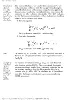
Confidence intervals for the true standard deviation can be constructed
using the chi-square distribution. The 100(1-
)% confidence intervals
that correspond to the tests of hypothesis on the previous page are given
by
Two-sided confidence interval for
1.
Lower one-sided confidence interval for
2.
Upper one-sided confidence interval for
3.
where for case (1) is the upper critical value from the
chi-square distribution with N-1 degrees of freedom and similarly for
cases (2) and (3). Critical values can be found in the chi-square table in
Chapter 1.
Choice of
risk level
can change
the
conclusion
Confidence interval (1) is equivalent to a two-sided test for the standard
deviation. That is, if the hypothesized or nominal value,
, is not
contained within these limits, then the hypothesis that the standard
deviation is equal to the nominal value is rejected.
7.2.3.1. Confidence interval approach
(1 of 2) [5/1/2006 10:38:34 AM]
A dilemma
of
hypothesis

testing
A change in
can lead to a change in the conclusion. This poses a
dilemma. What should
be? Unfortunately, there is no clear-cut
answer that will work in all situations. The usual strategy is to set
small so as to guarantee that the null hypothesis is wrongly rejected in
only a small number of cases. The risk, , of failing to reject the null
hypothesis when it is false depends on the size of the discrepancy, and
also depends on
. The discussion on the next page shows how to
choose the sample size so that this risk is kept small for specific
discrepancies.
7.2.3.1. Confidence interval approach
(2 of 2) [5/1/2006 10:38:34 AM]
7. Product and Process Comparisons
7.2. Comparisons based on data from one process
7.2.3. Are the data consistent with a nominal standard deviation?
7.2.3.2.Sample sizes required
Sample sizes
to minimize
risk of false
acceptance
The following procedure for computing sample sizes for tests involving standard
deviations follows W. Diamond (1989). The idea is to find a sample size that is
large enough to guarantee that the risk,
, of accepting a false hypothesis is small.
Alternatives
are specific
departures

from the null
hypothesis
This procedure is stated in terms of changes in the variance, not the standard
deviation, which makes it somewhat difficult to interpret. Tests that are generally of
interest are stated in terms of
, a discrepancy from the hypothesized variance. For
example:
Is the true variance larger than its hypothesized value by
?1.
Is the true variance smaller than its hypothesized value by
?2.
That is, the tests of interest are:
H
0
: 1.
H
0
: 2.
Interpretation The experimenter wants to assure that the probability of erroneously accepting the
null hypothesis of unchanged variance is at most
. The sample size, N, required
for this type of detection depends on the factor,
; the significance level, ; and
the risk,
.
First choose
the level of
significance
and beta risk
The sample size is determined by first choosing appropriate values of

and and
then following the directions below to find the degrees of freedom,
, from the
chi-square distribution.
7.2.3.2. Sample sizes required
(1 of 5) [5/1/2006 10:38:35 AM]
The
calculations
should be
done by
creating a
table or
spreadsheet
First compute
Then generate a table of degrees of freedom, say between 1 and 200. For case (1) or
(2) above, calculate
and the corresponding value of for each value of
degrees of freedom in the table where
1.
2.
The value of
where is closest to is the correct degrees of freedom and
N = + 1
Hints on
using
software
packages to
do the
calculations
The quantity

is the critical value from the chi-square distribution with
degrees of freedom which is exceeded with probability . It is sometimes referred
to as the percent point function (PPF) or the inverse chi-square function. The
probability that is evaluated to get
is called the cumulative density function
(CDF).
Example Consider the case where the variance for resistivity measurements on a lot of
silicon wafers is claimed to be 100 ohm
.
cm. A buyer is unwilling to accept a
shipment if
is greater than 55 ohm
.
cm for a particular lot. This problem falls
under case (1) above. The question is how many samples are needed to assure risks
of
= 0.05 and = .01.
7.2.3.2. Sample sizes required
(2 of 5) [5/1/2006 10:38:35 AM]
Calculations
using
Dataplot
The procedure for performing these calculations using Dataplot is as follows:
let d=55
let var = 100
let r = 1 + d/(var)
let function cnu=chscdf(chsppf(.95,nu)/r,nu) - 0.01
let a = roots cnu wrt nu for nu = 1 200
Dataplot returns a value of 169.5. Therefore, the minimum sample size needed to
guarantee the risk level is N = 170.

Alternatively, we could generate a table using the following Dataplot commands:
let d=55
let var = 100
let r = 1 + d/(var)
let nu = 1 1 200
let bnu = chsppf(.95,nu)
let bnu=bnu/r
let cnu=chscdf(bnu,nu)
print nu bnu cnu for nu = 165 1 175
Dataplot
output
The Dataplot output, for calculations between 165 and 175 degrees of freedom, is
shown below.
VARIABLES
NU BNU CNU
0.1650000E+03 0.1264344E+03 0.1136620E-01
0.1660000E+03 0.1271380E+03 0.1103569E-01
0.1670000E+03 0.1278414E+03 0.1071452E-01
0.1680000E+03 0.1285446E+03 0.1040244E-01
0.1690000E+03 0.1292477E+03 0.1009921E-01
0.1700000E+03 0.1299506E+03 0.9804589E-02
0.1710000E+03 0.1306533E+03 0.9518339E-02
0.1720000E+03 0.1313558E+03 0.9240230E-02
0.1730000E+03 0.1320582E+03 0.8970034E-02
0.1740000E+03 0.1327604E+03 0.8707534E-02
0.1750000E+03 0.1334624E+03 0.8452513E-02
The value of
which is closest to 0.01 is 0.010099; this has degrees of freedom
= 169. Therefore, the minimum sample size needed to guarantee the risk level is
N = 170.

Calculations
using EXCEL
The procedure for doing the calculations using an EXCEL spreadsheet is shown
below. The EXCEL calculations begin with 1 degree of freedom and iterate to the
correct solution.
7.2.3.2. Sample sizes required
(3 of 5) [5/1/2006 10:38:35 AM]
Definitions in
EXCEL
Start with:
1 in A11.
CHIINV{(1-
), A1}/R in B12.
CHIDIST(B1,A1) in C1
In EXCEL, CHIINV{(1-
), A1} is the critical value of the chi-square
distribution that is exceeded with probabililty
. This example requires
CHIINV(.95,A1). CHIDIST(B1,A1) is the cumulative density function up to
B1 which, for this example, needs to reach 1 -
= 1 - 0.01 = 0.99. The
EXCEL screen is shown below.
3.
7.2.3.2. Sample sizes required
(4 of 5) [5/1/2006 10:38:35 AM]
Iteration step Then:
From TOOLS, click on "GOAL SEEK"1.
Fill in the blanks with "Set Cell C1", "To Value 1 -
" and "By Changing
Cell A1".

2.
Click "OK"3.
Clicking on "OK" iterates the calculations until C1 reaches 0.99 with the
corresponding degrees of freedom shown in A1:
7.2.3.2. Sample sizes required
(5 of 5) [5/1/2006 10:38:35 AM]
7. Product and Process Comparisons
7.2. Comparisons based on data from one process
7.2.4.Does the proportion of defectives
meet requirements?
Testing
proportion
defective is
based on the
binomial
distribution
The proportion of defective items in a manufacturing process can be
monitored using statistics based on the observed number of defectives
in a random sample of size N from a continuous manufacturing
process, or from a large population or lot. The proportion defective in
a sample follows the binomial distribution where p is the probability
of an individual item being found defective. Questions of interest for
quality control are:
Is the proportion of defective items within prescribed limits?1.
Is the proportion of defective items less than a prescribed limit?2.
Is the proportion of defective items greater than a prescribed
limit?
3.
Hypotheses
regarding

proportion
defective
The corresponding hypotheses that can be tested are:
p = p
0
1.
p p
0
2.
p
p
0
3.
where p
0
is the prescribed proportion defective.
Test statistic
based on a
normal
approximation
Given a random sample of measurements Y
1
, , Y
N
from a population,
the proportion of items that are judged defective from these N
measurements is denoted . The test statistic
depends on a normal approximation to the binomial distribution that is
valid for large N, (N > 30). This approximation simplifies the
calculations using critical values from the table of the normal

distribution as shown below.
7.2.4. Does the proportion of defectives meet requirements?
(1 of 3) [5/1/2006 10:38:35 AM]
Restriction on
sample size
Because the test is approximate, N needs to be large for the test to be
valid. One criterion is that N should be chosen so that
min{Np
0
, N(1 - p
0
)} >= 5
For example, if p
0
= 0.1, then N should be at least 50 and if p
0
= 0.01,
then N should be at least 500. Criteria for choosing a sample size in
order to guarantee detecting a change of size
are discussed on
another page.
One and
two-sided
tests for
proportion
defective
Tests at the 1 -
confidence level corresponding to hypotheses (1),
(2), and (3) are shown below. For hypothesis (1), the test statistic,
z, is

compared with
, the upper critical value from the normal
distribution that is exceeded with probability and similarly for (2)
and (3). If
1.
2.
3.
the null hypothesis is rejected.
Example of a
one-sided test
for proportion
defective
After a new method of processing wafers was introduced into a
fabrication process, two hundred wafers were tested, and twenty-six
showed some type of defect. Thus, for N= 200, the proportion
defective is estimated to be
= 26/200 = 0.13. In the past, the
fabrication process was capable of producing wafers with a proportion
defective of at most 0.10. The issue is whether the new process has
degraded the quality of the wafers. The relevant test is the one-sided
test (3) which guards against an increase in proportion defective from
its historical level.
Calculations
for a
one-sided test
of proportion
defective
For a test at significance level
= 0.05, the hypothesis of no
degradation is validated if the test statistic

z is less than the critical
value, z
.05
= 1.645. The test statistic is computed to be
7.2.4. Does the proportion of defectives meet requirements?
(2 of 3) [5/1/2006 10:38:35 AM]
Interpretation Because the test statistic is less than the critical value (1.645), we
cannot reject hypothesis (3) and, therefore, we cannot conclude that
the new fabrication method is degrading the quality of the wafers. The
new process may, indeed, be worse, but more evidence would be
needed to reach that conclusion at the 95% confidence level.
7.2.4. Does the proportion of defectives meet requirements?
(3 of 3) [5/1/2006 10:38:35 AM]
7. Product and Process Comparisons
7.2. Comparisons based on data from one process
7.2.4. Does the proportion of defectives meet requirements?
7.2.4.1. Confidence intervals
Confidence
intervals
using the
method of
Agresti and
Coull
The method recommended by Agresti and Coull (1998) and also by
Brown, Cai and DasGupta (2001) (the methodology was originally
developed by Wilson in 1927) is to use the form of the confidence
interval that corresponds to the hypothesis test given in Section 7.2.4.
That is, solve for the two values of p
0
(say, p

upper
and p
lower
) that result
from setting z =
and solving for p
0
= p
upper
, and then setting z = -
and solving for p
0
= p
lower
. (Here, as in Section 7.2.4, denotes
the variate value from the standard normal distribution such that the area
to the right of the value is
/2.) Although solving for the two values of
p
0
might sound complicated, the appropriate expressions can be
obtained by straightforward but slightly tedious algebra. Such algebraic
manipulation isn't necessary, however, as the appropriate expressions
are given in various sources. Specifically, we have
Formulas
for the
confidence
intervals
Procedure
does not

strongly
depend on
values of p
and n
This approach can be substantiated on the grounds that it is the exact
algebraic counterpart to the (large-sample) hypothesis test given in
section 7.2.4 and is also supported by the research of Agresti and Coull.
One advantage of this procedure is that its worth does not strongly
depend upon the value of n and/or p, and indeed was recommended by
Agresti and Coull for virtually all combinations of n and p.
7.2.4.1. Confidence intervals
(1 of 9) [5/1/2006 10:38:37 AM]
Another
advantage is
that the
lower limit
cannot be
negative
Another advantage is that the lower limit cannot be negative. That is not
true for the confidence expression most frequently used:
A confidence limit approach that produces a lower limit which is an
impossible value for the parameter for which the interval is constructed
is an inferior approach. This also applies to limits for the control charts
that are discussed in Chapter 6.
One-sided
confidence
intervals
A one-sided confidence interval can also be constructed simply by
replacing each
by in the expression for the lower or upper limit,

whichever is desired. The 95% one-sided interval for p for the example
in the preceding section is:
Example
p
lower limit
p 0.09577
Conclusion
from the
example
Since the lower bound does not exceed 0.10, in which case it would
exceed the hypothesized value, the null hypothesis that the proportion
defective is at most .10, which was given in the preceding section,
would not be rejected if we used the confidence interval to test the
hypothesis. Of course a confidence interval has value in its own right
and does not have to be used for hypothesis testing.
Exact Intervals for Small Numbers of Failures and/or Small Sample
Sizes
7.2.4.1. Confidence intervals
(2 of 9) [5/1/2006 10:38:37 AM]