Báo cáo hóa học: "Research Article Two-Step Time of Arrival Estimation for Pulse-Based Ultra-Wideband Systems" potx

Hindawi Publishing Corporation
EURASIP Journal on Advances in Signal Processing
Volume 2008, Article ID 529134, 11 pages
doi:10.1155/2008/529134
Research Article
Two-Step Time of Arrival Estimation for
Pulse-Based Ultra-Wideband Systems
Sinan Gezici,
1
Zafer Sahinoglu,
2
Andreas F. Molisch,
2
Hisashi Kobayashi,
3
and H. Vincent Poor
3
1
Department of Electrical and Electronics Engineering, Bilkent University, Bilkent, Ankara 06800, Turkey
2
Mitsubishi Electric Research Labs, 201 Broadway, Cambridge, MA 02139, USA
3
Department of Electrical Engineering, Princeton University, Princeton, NJ 08544, USA
Correspondence should be addressed to Sinan Gezici,
Received 12 November 2007; Revised 12 March 2008; Accepted 14 April 2008
Recommended by Davide Dardari
In cooperative localization systems, wireless nodes need to exchange accurate position-related information such as time-of-arrival
(TOA) and angle-of-arrival (AOA), in order to obtain accurate location information. One alternative for providing accurate
position-related information is to use ultra-wideband (UWB) signals. The high time resolution of UWB signals presents a potential
for very accurate positioning based on TOA estimation. However, it is challenging to realize very accurate positioning systems in
practical scenarios, due to both complexity/cost constraints and adverse channel conditions such as multipath propagation. In this

paper, a two-step TOA estimation algorithm is proposed for UWB systems in order to provide accurate TOA estimation under
practical constraints. In order to speed up the estimation process, the first step estimates a coarse TOA of the received signal based
on received signal energy. Then, in the second step, the arrival time of the first signal path is estimated by considering a hypothesis
testing approach. The proposed scheme uses low-rate correlation outputs and is able to perform accurate TOA estimation in
reasonable time intervals. The simulation results are presented to analyze the performance of the estimator.
Copyright © 2008 Sinan Gezici et al. This is an open access article distributed under the Creative Commons Attribution License,
which permits unrestricted use, distribution, and reproduction in any medium, provided the original work is properly cited.
1. INTRODUCTION
Recently, communications, positioning, and imaging systems
that employ ultra-wideband (UWB) signals have drawn
considerable attention [1–5]. Commonly, a UWB signal is
defined to be one that possesses an absolute bandwidth of
at least 500 MHz or a relative bandwidth larger than 20%.
The main feature of a UWB signal is that it can coexist with
incumbent systems in the same frequency range due to its
large spreading factor and low power spectral density. UWB
technology holds great promise for a variety of applications
such as short-range, high-speed data transmission and
precise position estimation [2, 6].
A common technique to implement a UWB commu-
nications system is to transmit very short-duration pulses
with a low duty cycle [7–11]. Such a system, called impulse
radio (IR), sends a train of pulses per information symbol
and usually employs pulse position modulation (PPM) or
binary-phase shift keying (BPSK) depending on the positions
or the polarities of the pulses, respectively. In order to
prevent catastrophic collisions among pulses of different
users and thus provide robustness against multiple access
interference (MAI), each information symbol is represented
by a sequence of pulses; the positions of the pulses within that

sequence are determined by a pseudo-random time hopping
(TH) sequence specific to each user [7].
In addition to communications systems, UWB signals are
also well suited for applications that require accurate position
information such as inventory control, search and rescue,
and security [3, 12]. They are also useful in the context of
cooperative localization systems, since exchange of accurate
position-related information is very important for efficient
cooperation. In the presence of inaccurate position-related
information, cooperation could be harmful by reducing
the localization accuracy. Therefore, high TOA estimation
accuracy of UWB signals is very desirable in cooperative
localization systems. Due to their penetration capability and
high time resolution, UWB signals can facilitate very precise
positioning based on time-of-arrival (TOA) estimation, as
suggested by the Cramer-Rao lower bound (CRLB) [3].
2 EURASIP Journal on Advances in Signal Processing
However, in practical systems, the challenge is to perform
precise TOA estimation in a reasonable time interval under
complexity/cost constraints [13].
Maximum likelihood (ML) approaches to TOA estima-
tion of UWB signals can get quite close to the theoretical
limits for high signal-to-noise ratios (SNRs) [14, 15].
However, they generally require joint optimization over a
large number of unknown parameters (channel coefficients
and delays for multipath components). Hence, they have
prohibitive complexity for practical applications. In [16], a
generalized maximum likelihood (GML) estimation prin-
ciple is employed to obtain iterative solutions after some
simplifications of the ML approach. However, this approach

still requires very high sampling rates, which is not suitable
for low-power and low-cost applications.
On the other hand, the conventional correlation-based
TOA estimation algorithms are both suboptimal and require
exhaustive search among thousands of bins, which results
in very slow TOA estimation [17, 18]. In order to speed up
the process, differentsearchstrategiessuchasrandomsearch
orbitreversalsearchareproposedin[19]. However, TOA
estimation time can still be quite high in certain scenarios.
In addition to the correlation-based TOA estimation, TOA
estimation based on energy detection provides a low-
complexity alternative, but this commonly comes at the price
of reduced accuracy [20, 21].
In the presence of multipath propagation, the first
incoming signal path, the delay of which determines the
TOA, may not be the strongest multipath component.
Therefore, instead of peak selection algorithms, first path
detection algorithms are commonly employed for UWB
TOA estimation [16, 21–25]. A common technique for first
path detection is to determine the first signal component
that is stronger than a specific threshold [25]. Alternatively,
the delay of the first path can be estimated based on
the signal path that has the minimum delay among a
subset of signal paths that are stronger than a certain
threshold [24]. Although TOA estimation gets more robust
against the effects of multipath propagation in both cases,
TOA estimation can still take a long time. Finally, a low-
complexity timing offset estimation technique, called timing
with dirty templates (TDT), is proposed in [23, 26–28],
which employs “dirty templates” in order to obtain timing

information based on symbol-rate samples. Although this
algorithm provides timing information at low complexity
and in short time intervals, the TOA estimate obtained from
the algorithm has an ambiguity equal to the extent of the
noise-only region between consecutive symbols.
One of the most challenging issues in UWB TOA
estimation is to obtain a reliable estimate in a reasonable
time interval under a constraint on sampling rate. In order
to have a low-power and low-complexity receiver, one should
assume low sampling rates at the output of the correlators.
However, when low-rate samples are employed, the TOA
estimation can take a very long time. Therefore, we propose
a two-step TOA estimation algorithm that can perform
TOA estimation from low-rate samples (typically on the
order of hundreds times slower sampling rate than chip-rate
sampling) in a reasonable time interval. In order to speed
up the estimation process, the first step estimates the coarse
TOA of the received signal based on received signal energy.
After the first step, the uncertainty region for TOA is reduced
significantly. Then, in the second step, the arrival time of the
first signal path is estimated based on low-rate correlation
outputs by considering a hypothesis testing approach. In
other words, the second step provides a fine TOA estimate by
using a statistical change detection approach. In addition, the
proposed algorithm can operate without any thresholding
operation, which increases its practicality.
The remainder of the paper is organized as follows.
Section 2 describes the transmitted and received signal
models in a frequency-selective environment. The two-step
TOA estimation algorithm is considered in Section 3,where

the algorithm is described in detail, and probability of
detection analysis is presented. Then, simulation results and
numericalstudiesarepresentedinSection 4, and concluding
remarks are made in Section 5.
2. SIGNAL MODEL
Consider a TH-IR system which transmits the following sig-
nal:
s
tx
(t) =
√
E
∞

j=−∞
a
j
b
j/N
f

w
tx

t − jT
f
−c
j
T
c


,(1)
where w
tx
(t) is the transmitted UWB pulse with duration T
c
;
E is the transmitted pulse energy; T
f
is the “frame” interval;
and b
j/N
f

∈{+1, −1} is the binary information symbol.
In order to smooth the power spectrum of the transmitted
signal and allow the channel to be shared by many users
without causing catastrophic collisions, a TH sequence c
j
∈
{
0, 1, , N
c
− 1} is assigned to each user, where N
c
is the
number of chips per frame interval, that is, N
c
= T
f

/T
c
.
Additionally, random polarity codes, a
j
’s, can be employed,
which are binary random variables taking on the values
±1
with equal probability, and are known to the receiver. Use of
random polarity codes helps reduce the spectral lines in the
power spectral density of the transmitted signal [29, 30]and
mitigate the effects of MAI [31, 32].
It can be shown that the signal model in (1) also covers
the signal structures employed in the preambles of IEEE
802.15.4a systems [2, 33].
The transmitted signal in (1) passes through a channel
with channel impulse response h(t), which is modeled as a
tapped-delay-line channel with multipath resolution T
c
as
follows [34–36]:
h(t)
=
L

l=1
α
l
δ


t −(l − 1)T
c
−τ
TOA

,(2)
where α
l
is the channel coefficient for the lth path; L is the
number of multipath components; and τ
TOA
is the TOA of
the incoming signal. Since the main purpose is to estimate
TOA with a chip-level uncertainty, the equivalent channel
model with resolution T
c
is employed.
Sinan Gezici et al. 3
From (1)and(2), and including the effects of the
antennas, the received signal can be expressed as
r(t)
=
L

l=1
√
Eα
l
s
rx


t −(l − 1)T
c
−τ
TOA

+ n(t), (3)
where n(t) is zero-mean white Gaussian noise with spectral
density σ
2
;ands
rx
(t)isgivenby
s
rx
(t) =
∞

j=−∞
a
j
b
j/N
f

w
rx

t − jT
f

−c
j
T
c

,(4)
with w
rx
(t) denoting the received UWB pulse with unit
energy.
Since TOA estimation is commonly performed at the
preamble section of a packet [33], we assume a data aided
TOA estimation scheme and consider a training sequence of
b
j
= 1 ∀j.Then,s
rx
(t)in(4) can be expressed as
s
rx
(t) =
∞

j=−∞
a
j
w
rx

t − jT

f
−c
j
T
c

. (5)
It is assumed, for simplicity, that the signal always arrives
in one frame duration (τ
TOA
<T
f
), and there is no interframe
interference (IFI), that is, T
f
≥ (L + c
max
)T
c
(equivalently,
N
c
≥ L + c
max
), where c
max
is the maximum value of the
TH sequence. Note that the assumption of τ
TOA
<T

f
does
not restrict the validity of the algorithm. In fact, it is enough
to have τ
TOA
<T
s
,whereT
s
is the symbol interval, for the
algorithm to work when the frame interval is large enough
and predetermined TH codes are employed. (In fact, in IEEE
802.15.4a systems, no TH codes are used in the preamble
section; hence, it is easy to extend the results to the τ
TOA
>T
f
case for those scenarios [2].) Moreover, even if τ
TOA
≥ T
s
,
an initial energy detection can be used to determine the
arrival time within a symbol uncertainty before running
the proposed algorithm. Finally, since a single-user scenario
is considered, c
j
= 0 ∀j can be assumed without loss of
generality.
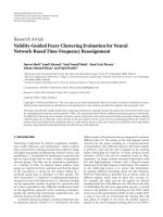
3. TWO-STEP TOA ESTIMATION ALGORITHM

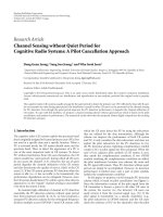
A TOA estimation algorithm provides an estimate for the
delay of an incoming signal, which is commonly obtained in
multiple steps, as shown in Figure 1. First, frame acquisition
is achieved in order to confine the TOA into an uncertainty
region of one frame interval (see [37]). Then, the TOA is
estimated with a chip-level uncertainty by a TOA estimation
algorithm, which is shown in the dashed box in Figure 1.
Then, the tracking unit provides subchip resolution by
employing a delay lock loop (DLL), which yields the final
TOA estimate [38–40]. The focus of this paper is on the two-
step TOA estimation algorithm shown in Figure 1.
In order to perform fast TOA estimation, the first step
of the proposed two-step TOA estimation algorithm obtains
a coarse TOA of the received signal based on received signal
energy. Then, in the second step, the arrival time of the first
signal path is estimated by considering a hypothesis testing
approach.
Frame
acquisition
Coarse TOA
estimation
Fine TOA
estimation
Tracking
Figure 1: Block diagram for TOA estimation. The algorithm in this
paper focuses on the blocks in the dashed box.
First, the TOA τ
TOA
in (3) is expressed as
τ

TOA
= kT
c
= k
b
T
b
+ k
c
T
c
,(6)
where k
∈ [0, N
c
−1] is the TOA in terms of the chip interval
T
c
; T
b
is the block interval consisting of B chips (T
b
= BT
c
);
and k
b
∈ [0, N
c
/B − 1] and k

c
∈ [0, B − 1] are the integers
that determine, respectively, in which block and chip the first
signal path arrives. Note that N
c
/B represents the number of
blocks, which is denoted by N
b
in the sequel.
The two-step TOA algorithm first estimates the block in
which the first signal path exists. Then, it estimates the chip
position in which the first path resides. In other words, it can
be summarized as follows:
(i) estimation of k
b
from received signal strength (RSS)
measurements;
(ii) estimation of k
c
(equivalently, k) from low-rate cor-
relation outputs using a hypothesis testing approach.
Note that the number of blocks N
b
(or the block length
T
b
) is an important design parameter. Selection of a smaller
block decreases the amount of time for TOA estimation
in the second step, since a smaller uncertainty region is
searched. On the other hand, smaller block sizes can result

in more errors in the first step since noise becomes more
effective. The optimal block size is affected by the SNR and
the channel characteristics.
3.1. First step: coarse TOA estimation based on
RSS measurements
In the first step, the aim is to detect the coarse arrival time
of the signal in the frame interval. Assume, without loss of
generality, that the frame time T
f
is an integer multiple of T
b
,
the block size of the algorithm, that is, T
f
= N
b
T
b
.
In order to have reliable decision variables in this step,
energy is combined from N
1
different frames of the incoming
signal for each block. Hence, the decision variables are
expressed as
Y
i
=
N
1

−1

j=0
Y
i,j
(7)
for i
= 0, , N
b
−1, where
Y
i,j
=

jT
f
+(i+1)T
b
jT
f
+iT
b


r(t)


2
dt. (8)
Then, k

b
in (6) is estimated as

k
b
= arg max
0≤i≤N
b
−1
Y
i
. (9)
4 EURASIP Journal on Advances in Signal Processing
In other words, the block with the largest signal energy is
selected.
The parameters of this step that should be selected
appropriately for accurate TOA estimation are the block size
T
b
(N
b
) and the number of frames N
1
, from which energy
is collected. In Section 3.4, the probability of selecting the
correct block will be quantified.
3.2. Second step: fine TOA estimation based on
low-rate correlation outputs
After determining the coarse arrival time in the first step,
the second step tries to estimate k

c
in (6). Ideally, k
c
∈
[0, B − 1] needs to be searched for TOA estimation, which
corresponds to searching k
∈ [

k
b
B,(

k
b
+1)B − 1] with

k
b
denoting the block index estimate in (9). However, in
some cases, the first signal path can reside in one of the
blocks prior to the strongest one due to multipath effects.
Therefore, instead of searching a single block, k
∈ [

k
b
B −
M
1
,(


k
b
+1)B − 1], with M
1
≥ 0, can be searched for the
TOA in order to increase the probability of detection of the
first path. In other words, in addition to the block with the
largest signal energy, an additional backwards search over
M
1
chips can be performed. For notational simplicity, let
U
={n
s
, n
s
+1, , n
e
}denote the uncertainty region, where
n
s
=

k
b
B − M
1
and n
e

= (

k
b
+1)B − 1 are the start and end
points.
In order to estimate the TOA with chip-level resolution,
correlations of the received signal with shifted versions of a
template signal are considered. For delay iT
c
, the following
correlation output is obtained:
z
i
=

iT
c
+N
2
T
f
iT
c
r(t)s
temp

t −iT
c


dt, (10)
where N
2
is the number of frames over which the correlation
output is obtained, and s
temp
(t) is the template signal given
by
s
temp
(t) =
N
2
−1

j=0
a
j
w
rx

t − jT
f

. (11)
Note that in practical systems, the received pulse shape may
not be known exactly, since the transmitted pulse can be
distorted by the channel. In those cases, if the system employs
w
tx

(t) instead of w
rx
(t) to construct the template signal in
(11), the system performance can degrade. In some cases,
that degradation may not be very significant [41]. For other
cases, template design techniques should be considered in
order to maintain a reasonable performance level [41, 42].
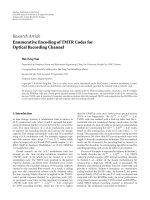
From the correlation outputs for different delays, the
aim is to determine the chip in which the first signal path
has arrived. By appropriate choice of the block interval
T
b
and M
1
, and considering a large number of multipath
components in the received signal, which is typical for
indoor UWB systems, it can be assumed that the block starts
with a number of chips with noise-only components and
the remaining ones with signal-plus-noise components, as
N
b
−1
T
b
T
f
T
c
N
b

···123
Figure 2: Illustration of the two-step TOA estimation algorithm.
The signal on the top is the received signal in one frame. The first
step checks the signal energy in N
b
blocks and chooses the one
with the highest energy (although one frame is shown in the figure,
energy from different frames can be collected for reliable decisions).
Assuming that the third block has the highest energy, the second
step focuses on this block (or an extension of that) to estimate the
TOA. The zoomed version of the signal in the third block is shown
on the bottom.
shown in Figure 2. Assuming that the statistics of the signal
paths do not change significantly in the uncertainty region
U, the different hypotheses can be expressed approximately
as follows:
H
0
: z
i
= η
i
, i = n
s
, , n
f
,
H
k
: z

i
= η
i
, i = n
s
, , k −1,
z
i
= N
2
√
Eα
i−k+1
+ η
i
, i = k, , n
f
,
(12)
for k
∈ U,whereH
0
is the hypothesis that all the
samples are noise samples; H
k
is the hypothesis that the
signal starts at the kth output; η
i
’s denote the independent
and identically distributed (i.i.d.) Gaussian output noise;

N (0, σ
2
n
)withσ
2
n
= N
2
σ
2
, α
1
, , α
n
f
−k+1
are independent
channel coefficients, assuming n
f
− n
s
+1 ≤ L,andn
f
=
n
e
+ M
2
with M
2

being the number of additional correlation
outputs that are considered out of the uncertainty region in
order to have reliable estimates of the unknown parameters
related to the channel coefficients.
Due to very time high resolution of UWB signals, it is
appropriate to model the channel coefficients approximately
as
α
1
= d
1


α
1


,
α
l
=
⎧
⎪
⎨
⎪
⎩
d
l



α
l


, p,
0, 1
− p,
l
= 2, ,n
f
−n
s
+1,
(13)
where p is the probability that a channel tap arrives in a given
chip; d
l
is the sign of α
l
,whichis±1 with equal probability;
Sinan Gezici et al. 5
and |α
l
| is the amplitude of α
l
, which is modeled as a
Nakagami-m distributed random variable with parameter Ω,
that is [43],
p(α)
=

2
Γ(m)

m
Ω

m
α
2m−1
e
−mα
2
/Ω
, (14)
for α
≥ 0, m ≥ 0.5, and Ω ≥ 0, where Γ(·) is the Gamma
function [44].
From the formulation in (12), it is observed that the TOA
estimation problem can be considered as a change detection
problem [45]. Let θ denote the unknown parameters of the
distribution of α, that is, θ
= [pmΩ]. Then, the log-
likelihood ratio (LLR) is given by
S
n
f
k
(θ) =
n
f


i=k
log
p
θ

z
i
| H
k

p

z
i
| H
0

, (15)
where p
θ
(z
i
| H
k
) denotes the probability density function
(p.d.f.) of the correlation output under hypothesis H
k
and
with unknown parameters given by θ,andp(z

i
| H
0
)denotes
the p.d.f. of the correlation output under hypothesis H
0
.
Since θ is unknown, its ML estimate can be obtained first
for a given hypothesis H
k
and then that estimate can be used
in the LLR expression. In other words, the generalized LLR
approach [45, 46] can be taken, where the TOA estimate is
expressed as

k = arg max
k∈U
S
n
f
k


θ
ML
(k)

(16)
with


θ
ML
(k) = arg sup
θ
S
n
f
k
(θ). (17)
However, the ML estimate is usually very complex to
calculate. Therefore, simpler estimators such as the method
of moments (MM) estimator can be employed to obtain
those parameters. The nth moment of a random variable X
having Nakagami-m distribution with parameter Ω is given
by
E

X
n

=
Γ(m + n/2)
Γ(m)

Ω
m

n/2
. (18)
Then, from the correlator outputs

{z
i
}
n
f
i=k+1
, the MM esti-
mates for the unknown parameters can be obtained after
some manipulation as
p
MM
=
γ
1
γ
2
2γ
2
2
−γ
3
, m
MM
=
2γ
2
2
−γ
3
γ

3
−γ
2
2
, Ω
MM
=
2γ
2
2
−γ
3
γ
2
,
(19)
where
γ
1
Δ
=
1
EN
2
2

μ
2
−σ
2

n

,
γ
2
Δ
=
1
E
2
N
4
2

μ
4
−3σ
4
n
γ
1
−6EN
2
2
σ
2
n

,
γ

3
Δ
=
1
E
3
N
6
2

μ
6
−15σ
6
n
γ
1
−15E
2
N
4
2
γ
2
σ
2
n
−45EN
2
2

σ
4
n

,
(20)
with μ
j
denoting the jth sample moment given by
μ
j
=
1
n
f
−k
n
f

i=k+1
z
j
i
. (21)
Then, the index of the chip having the first signal path
can be obtained as

k = arg max
k∈U
S

n
f
k


θ
MM
(k)

, (22)
where θ
MM
(k) = [p
MM
m
MM
Ω
MM
] is the MM estimate
for the unknown parameters. Note that the dependence of
p
MM
, m
MM
,andΩ
MM
on the change position k is not shown
explicitly for notational simplicity.
Let p
1

(z)andp
2
(z), respectively, denote the distributions
of η and N
2
√
Ed|α|+η. Then, the generalized LLR for the kth
hypothesis can be obtained as
S
n
f
k
(

θ) = log
p
2

z
k

p
1

z
k

+
n
f


i=k+1
log
pp
2

z
i

+(1− p)p
1

z
i

p
1

z
i

,
(23)
where
p
1
(z) =
1
√
2πσ

n
e
−z
2
/2σ
2
n
,
(24)
p
2
(z) =
ν
1
√
2πσ
n
e
−z
2
/2σ
2
n
Φ

m,
1
2
;
z

2
ν
2

(25)
with
ν
1
Δ
=
2
√
πΓ(2m)
Γ(m)Γ(m +0.5)

4+
2EN
2
2
Ω
mσ
2
n

−m
,
ν
2
Δ
= 2σ

2
n

1+2m
σ
2
n
EN
2
2
Ω

,
(26)
and Φ denoting a confluent hypergeometric function given
by [44]:
Φ

β
1
, β
2
; x

= 1+
β
1
β
2
x

1!
+
β
1

β
1
+1

β
2

β
2
+1

x
2
2!
+
β
1

β
1
+1

β
1
+2


β
2

β
2
+1

β
2
+2

x
3
3!
+
···.
(27)
Note that the p.d.f. of N
2
√
Ed|α| + η, p
2
(z) is obtained
from (14), (24), and the fact that d is
±1withequal
probability.
After some manipulation, the TOA estimation rule can
be expressed as


k = arg max
k∈U

log

ν
1
Φ

m,0.5;
z
2
k
ν
2

+
n
f

i=k+1
log

pν
1
Φ

m,0.5;
z
2

i
ν
2

+1− p


.
(28)
Note that this estimation rule does not require any threshold
setting, since it obtains the TOA estimate as the chip index
that maximizes the decision variable in (28).
6 EURASIP Journal on Advances in Signal Processing
3.3. Additional tests
The formulation in (12) assumes that the block always
starts with noise-only components, and then the signal paths
start to arrive. However, in practice, there can be cases in
which the first step chooses a block consisting of all noise
components. By combining a large number of frames, that
is, by choosing a large N
1
in (7), the probability of this
event can be reduced considerably. However, very large N
1
also increases the estimation time. Hence, there is a trade-
off between the estimation error and the estimation time. In
order to prevent erroneous TOA estimation when a noise-
only block is chosen, a one-sided test can be applied using
the known distribution of the noise outputs. Since the noise
outputs have a Gaussian distribution, the test reduces to the

comparison of the average energy of the outputs after the
estimated change instant against a threshold. In other words,
if (1/(n
f
−

k +1))

n
f
i=

k
z
2
i
<δ
1
, the block is considered as a
noise-only block and the two-step algorithm is run again.
Another improvement of the algorithm can be obtained
by checking if the block consists of all signal paths, that is,
the TOA is prior to the current block. Again, by following
a one-sided test approach, we can check the average energy
of the correlation outputs before the estimated TOA against
a threshold and detect an all-signal block if the threshold
is exceeded. However, for very small values of the TOA
estimate

k, there can be a significant probability that the

first signal path arrives before the current observation region
since the distribution of the correlation output after the first
path includes both the noise distribution and the signal-
plus-noise distribution with some probabilities as shown in
(13). Hence, the test may fail although the block is an all-
signal block. Therefore, some additional correlation outputs
before

k can be employed as well, when calculating the
average power before the TOA estimate. In other words, if
(1/(

k − n
s
+ M
3
))


k−1
i
=n
s
−M
3
z
2
i
>δ
2

, the block is considered
as an all-signal block, where M
3
≥ 0 additional outputs are
used depending on

k. When it is determined that the block
consists of all signal outputs, the TOA is expected to be in
one of the previous blocks. Therefore, the uncertainty region
is shifted backwards, and the change detection algorithm is
repeated.
3.4. Probability of block detection
In the proposed two-step TOA estimator, determination of
the block that contains the first signal path carries significant
importance. Therefore, in this section, the probability of
selecting the correct block is analyzed in detail.
Let the received signal in the ith block of the jth frame be
denoted by r
i,j
(t), that is,
r
i,j
(t)
.
=
⎧
⎪
⎨
⎪
⎩

r(t), t ∈

jT
f
+ iT
b
, jT
f
+(i +1)T
b

,
0, otherwise
(29)
for i
= 0, 1, , N
b
− 1, and j = 0, 1, , N
1
− 1. Under
the assumption that the channel impulse response does not
change during at least N
1
frame intervals, r
i,j
(t)canbe
expressed as
r
i,j
(t) = s

i
(t)+n
i,j
(t), (30)
where s
i
(t) is the signal part in the ith block, and n
i,j
(t) is the
noise in the ith block of the jth frame. Note that due to the
static channel assumption, the signal part is identical for the
ith block of all N
1
frames. In addition, the noise components
are independent for different block and/or frame indices.
From (29)and(30), the signal energy in (8)canbe
expressed as
Y
i,j
=

∞
−∞


r
i,j
(t)



2
dt, (31)
which becomes
Y
i,j
=

∞
−∞


n
i,j
(t)


2
dt, (32)
for noise-only blocks, and
Y
i,j
=

∞
−∞


s
i
(t)+n

i,j
(t)


2
dt, (33)
for signal-plus-noise blocks, that is, for blocks that contain
some signal components in addition to noise. It can be
shown that Y
i,j
has a central or noncentral chi-square
distribution depending on the type of the block. Let B
n
and
B
s
represent the sets of block indices for noise-only and
signal-plus-noise blocks, respectively. Then,
Y
i,j
∼
⎧
⎪
⎨
⎪
⎩
χ
2
n
(0), i ∈ B

n
,
χ
2
n
(ε
i
), i ∈ B
s
,
(34)
where n is the approximate dimensionality of the signal
space, which is obtained from the time-bandwidth product
[47]; ε
i
is the energy of the signal in the ith block;
ε
i
=

|
s
i
(t)|
2
dt;andχ
2
n
(ε) denotes a noncentral chi-square
distribution with n degrees of freedom and a noncentrality

parameter of ε. Clearly, χ
2
n
(ε)reducestoacentralchi-square
distribution with n degrees of freedom for noise-only blocks
for which ε
= 0.
As expressed in (7), each decision variable for block
estimation is obtained by adding signal energy from N
1
frames. From the fact that the sum of i.i.d. noncentral chi-
square random variables with n degrees of freedom and with
noncentrality parameter ε results in another noncentral chi-
square random variable with N
1
n degrees of freedom and
noncentrality parameter N
1
ε, the probability distribution of
Y
i
in (7) can be expressed as
Y
i
=
N
1
−1

j=0

Y
i,j
∼
⎧
⎪
⎨
⎪
⎩
χ
2
N
1
n
(0), i ∈ B
n
,
χ
2
N
1
n

N
1
ε
i

, i ∈ B
s
.

(35)
The probability that the TOA estimator selects the lth
block, which is a signal-plus-noise block, as the block that
contains the first signal path is given by
P
l
D
= Pr

Y
l
>Y
i
, ∀i
/
=l

(36)
Sinan Gezici et al. 7
for l ∈ B
s
, which can be expressed as
P
l
D
=

∞
0
p

Y
l
(y)

i∈B
s
\{l}
Pr

Y
i
<y


j∈B
n
Pr

Y
j
<y

dy,
(37)
where p
Y
l
(y) represents the p.d.f. of the signal energy in the
lth block. Since the energies of the noise-only blocks are i.i.d.,
(37)becomes

P
l
D
=

∞
0
p
Y
l
(y)

Pr

Y
j
<y

|B
n
|

i∈B
s
\{l}
Pr

Y
i
<y


dy,
(38)
where
|B
n
| denotes the number of elements in set B
n
,andj
can be any value from B
n
. (It is also observed from (35) that
the p.d.f. of energy in a noise-only block does not depend on
the index of the block.)
From (35), (38) can be obtained, after some manipula-
tion, as in the appendix:
P
l
D
=
e
−N
1
ε/(2σ
2
)

2σ
2


|B
s
|

∞
0
f
l
(y)

1 −e
−y/(2σ
2
)
N
1
n/2−1

k=0
1
k!

y
2σ
2

k

|B
n

|
×

i∈B
s
\{l}

y
0
f
i
(x)dx dy,
(39)
where N
1
n is assumed to be an even number; ε =

i∈B
s
ε
i
represents the total signal energy; and
f
l
(y) = e
−y/(2σ
2
)

y

N
1
ε
l

(N
1
n−2)/4
I
N
1
n/2−1


N
1
ε
l
y
σ
2

(40)
with
I
κ
(x) =
∞

i=0

(x/2)
κ+2i
i!Γ(κ + i +1)
, x
≥ 0 (41)
representing the κth-order modified Bessel function of the
first kind, and Γ(
·) denoting the gamma function [48].
In the presence of a single signal-plus-noise block, that is,
B
s
={l},(39)reducesto
P
l
D
=
e
−N
1
ε
l
/(2σ
2
)
2σ
2

∞
0
f

l
(y)

1−e
−y/(2σ
2
)
N
1
n/2−1

k=0
1
k!

y
2σ
2

k

|B
n
|
dy,
(42)
which can be evaluated easily via numerical integration.
However, in the presence of multiple signal-plus-noise
blocks, numerical integration to calculate P
l

D
from (39)and
(40) can have high computational complexity. Therefore,
a Monte-Carlo approach can be followed, by generating a
number of noncentral chi-square distributed samples, and
by approximating the expectation operation in (38) by the
sample mean of the inner probability terms. Although the
probability of detecting block l can be calculated exactly
basedon(39)and(40), a simpler expression can be obtained
by means of Gaussian approximation for a large number of
frames. In other words, for large values of N
1
, Y
i
in (7)can
be approximated by a Gaussian random variable.
From (34), the Gaussian approximation can be obtained
as
Y
i
=
N
1
−1

j=0
Y
i,j
∼
⎧

⎨
⎩
N

N
1
nσ
2
,2N
1
nσ
4

, i ∈ B
n
,
N

N
1

nσ
2
+ε
i

,2N
1
σ
2


nσ
2
+2ε
i

, i ∈ B
s
.
(43)
Then, the probabilities that the energy of the lth block is
larger than that of the other signal-plus-noise blocks or than
the noise-only blocks are given, respectively, by
Pr

Y
i
<y

≈
Q

N
1

nσ
2
+ ε
i


−
y

2N
1
σ
2

nσ
2
+2ε
i


(44)
for i
∈ B
s
\{l},and
Pr

Y
j
<y

≈
Q

N
1

nσ
2
− y
σ
2

2N
1
n

(45)
for j
∈ B
n
,whereQ(x) = (1/
√
2π)

∞
x
e
−t
2
/2
dt represents
the Q-function. Note that the detection probability in (38)
can be calculated easily from (44)and(45)vianumerical
integration techniques. In addition, as will be investigated in
Section 4, the Gaussian approximation is quite accurate for
practical signal parameters.

Since the index of the block that includes the first signal
path is denoted by k
b
in Section 3, the probability that
the correct block is selected is given by P
k
b
D
, which can
be obtained from (38)–(45). If the TOA estimator searches
both the selected block and the previous block in order to
increase the probability that the first signal path is included
in the search space of the second step, then the probability
of including the first signal path in the search space of the
second step is given by P
k
b
D
+ P
k
b
+1
D
.
4. SIMULATION RESULTS
In this section, numerical studies and simulations are
performed in order to evaluate the expressions in Section 3.4,
and to investigate the performance of the proposed TOA
estimator over realistic IEEE 802.15.4a channel models [43,
49].

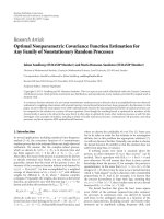
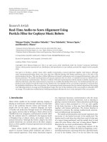
First, the expressions in Section 3.4 for probability of
block detection are investigated. Consider a scenario with
N
b
= 10 blocks, all of which are noise-only blocks except
for the fifth one. Also, the degrees of freedom for each
energy sample, n in (34), are taken to be 10. In Figure 3, the
probabilities of block detection are plotted versus SNR for
N
1
= 5andN
1
= 25, where N
1
is the number of frames over
which the energy samples are combined. SNR is defined as
the ratio between the total signal energy ε in the blocks and
σ
2
(Section 3.4). It is observed that the exact expression and
the one based on Gaussian approximation yield very close
values. Especially, for N
1
= 25, the results are in very good
8 EURASIP Journal on Advances in Signal Processing
151050−5−10−15
SNR (dB)
0
0.1
0.2

0.3
0.4
0.5
0.6
0.7
0.8
0.9
1
Probability of detection
Exact, N
1
= 5
Approx., N
1
= 5
Exact, N
1
= 25
Approx., N
1
= 25
Figure 3: Probability of block detection versus SNR for N
b
= 10,
n
= 10, and ε
i
= 0 ∀i
/
=5.

302520151050
SNR (dB)
0
0.1
0.2
0.3
0.4
0.5
0.6
0.7
0.8
0.9
1
Probability of detection
Exact, N
1
= 5
Approx., N
1
= 5
Exact, N
1
= 25
Approx., N
1
= 25
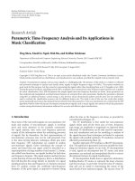
Figure 4: Probability of block detection versus SNR for N
b
= 20,
n

= 5, and ε = [3 2.521.25 0.5 0
15
].
agreement, as the Gaussian approximation becomes more
accurate as N
1
increases.
In Figure 4, the probability of block detections are
plotted versus SNR for N
b
= 20, n = 5, and ε =
[3 2.521.25 0.5 0
15
], where ε = [ε
1
···ε
N
b
], and 0
15
represents a row vector of 15 zeros. From the plot, it is
observed that the exact and approximate curves are in good
agreement as in the previous case. Also, due to the presence
of multiple signal blocks with close energy levels, higher SNR
values, than those in the previous case, are needed for reliable
detection of the first block in this scenario.
2520151050−5−10−15
SNR (dB)
0
0.1

0.2
0.3
0.4
0.5
0.6
0.7
0.8
0.9
1
Probability of block detection
λ = 0
λ
= 0.1
λ
= 1
λ
= 10
Figure 5: Probability of block detection versus SNR for ε
i
= e
−λ(i−1)
for i = 1, , N
b
, n = 10, N
1
= 25, and N
b
= 10.
Next, the block energies are modeled as exponentially
decaying, ε

i
= e
−λ(i−1)
for i = 1, , N
b
, and the block
detection probabilities are obtained for various decay factors,
for n
= 10, N
1
= 25, and N
b
= 10. In Figure 5,
better detection performance is observed as the decay factor
increases. In other words, if the energy of the first block is
considerably larger than the energies of the other blocks, the
probability of block detection increases. At the extreme case
in which all the blocks have the same energy, the probability
converges to 0.1, which is basically equal to the probability of
selecting one of the 10 blocks in a random fashion.
In order to investigate the performance of the proposed
estimator, residential and office environments with both line-
of-sight (LOS) and nonline-of-sight (NLOS) situations are
considered according to the IEEE 802.15.4a channel models
[43]. In the simulation scenario, the signal bandwidth is
7.5 GHz and the frame time of the transmitted training
sequence is 300 nanoseconds. Hence, an uncertainty region
consisting of 2250 chips is considered, and that region is
divided into N
b

= 50 blocks. In the proposed algorithm, the
numbers of pulses, over which the correlations are taken in
the first and second steps, are given by N
1
= 50 and N
2
= 25,
respectively. Also M
1
= 180 additional chips prior to the
uncertainty region determined by the first step are included
in the second step. The estimator is assumed to have 10
parallel correlators for the second step. In a practical setting,
the estimator can use the correlators of a Rake receiver that
is already present for the signal demodulation, and 10 is a
conservative value in this sense.
From the simulations, it is obtained that each TOA
estimation takes about 1 millisecond (0.92 millisecond to be
more precise). (Since we do not employ any additional tests
after the TOA estimate, which are described in Section 3.3,
and use the same parameters for all the channel models, the
estimation time is the same for all the channel realizations.)
Sinan Gezici et al. 9
2019181716151413121110
SNR (dB)
10
−2
10
−1
10

0
10
1
10
2
RMSE (m)
CM-1: residential LOS
CM-2: residential NLOS
CM-3: office LOS
CM-4: office NLOS
Proposed
Max. selection
MLE
Figure 6: RMSE versus SNR for the proposed and the conventional
maximum (peak) selection algorithms.
In order to have a fair comparison with the conventional
correlation-based peak selection algorithm, a training signal
duration of 1 millisecond is considered for that algo-
rithm as well. For both algorithms, frame-rate sampling
is assumed. In Figure 6, the root-mean-square errors are
plotted versus SNR for the proposed and the conventional
algorithms under four different channel conditions. Due to
the different characteristics of the channels in residential
and office environments, the estimates are better in the
office environment. Namely, the delay spread is smaller in
the channel models for the office environment. Moreover,
as expected, the NLOS situations cause increase in the
RMSE values. Comparison of the two algorithms reveal that
the proposed algorithm can provide better accuracy than
the conventional one. Especially, at high SNR values the

proposed algorithm can provide less than a meter accuracy
for LOS channels and about 2 meters accuracy for NLOS
channels. In addition to the conventional and the proposed
approaches, the maximum likelihood estimator (MLE) is
also illustrated in Figure 6 as a theoretical limit for CM-
3. For the MLE, it is assumed that Nyquist-rate samples of
the signal can be obtained over two frames and the channel
coefficients are known. Note that due to the impractical
assumptions related to the MLE, the lower limit provided
by the MLE is not tight. Therefore, it is concluded that
more realistic theoretical limits (e.g., CRLB) based on low-
rate noncoherent and coherent signal samples need to be
obtained, which are a topic of future research.
Note that one disadvantage of the conventional approach
is that it needs to search for TOA in every chip position
one by one. However, the proposed algorithm first employs
coarse TOA estimation, and therefore it can perform fine
TOA estimation only in a smaller uncertainty region. In
2019181716151413121110
SNR (dB)
10
−2
10
−1
10
0
10
1
10
2

RMSE (m)
CM-1: residential LOS
CM-2: residential NLOS
CM-3: office LOS
CM-4: office NLOS
Proposed
2-step max. selection
MLE
Figure 7: RMSE versus SNR for the proposed and the two-step peak
selection algorithms.
order to investigate how much the conventional algorithm
can be improved by applying a similar two-step approach,
a modified version of the conventional algorithm is consid-
ered, which first employs the coarse TOA estimation (via
energy detection), and then performs the conventional peak
selection in the second step. Figure 7 compares the proposed
algorithm with the modified version of the conventional
algorithm. Note from Figures 6 and 7 that the performance
of the conventional algorithm is slightly enhanced by
employing a two-step approach, since correlation outputs
can be obtained more reliably over the 1 millisecond training
signal interval for the latter. In other words, more time
can be allocated to the chip positions around the TOA
by applying the coarse TOA estimation first. However,
the performance is still considerably worse than that of
the proposed approach, since the peak selection in the
conventional approach performs significantly worse than the
proposed change detection technique.
Finally, note that for the proposed algorithm, the same
parameters are used for all the channel models. More

accurate results can be obtained by employing different
parameters in different scenarios. In addition, by applying
additional tests described in Section 3.3, the accuracy can be
enhanced even further.
5. CONCLUSIONS
In this paper, we have proposed a two-step TOA estimation
algorithm, where the first step uses RSS measurements
to quickly obtain a coarse TOA estimate, and the second
step uses a change detection approach to estimate the fine
TOA of the signal. The proposed scheme relies on low-rate
correlation outputs, but still obtains a considerably accurate
10 EURASIP Journal on Advances in Signal Processing
TOA estimate in a reasonable time interval, which makes it
quite practical for realistic UWB systems. Simulations have
been performed to analyze the performance of the proposed
TOA estimator, and the comparisons with the conventional
TOA estimation techniques have been presented.
APPENDIX
A. DERIVATION OF (39)
Since the energy is distributed according to noncentral chi-
square distribution for signal-plus-noise blocks, as specified
by (35), p
Y
l
(y)in(38)isgivenby
p
Y
l
(y) =
1

2σ
2

y
N
1
ε
l

(N
1
n−2)/4
e
−(y+N
1
ε
l
)/2σ
2
I
N
1
n/2−1


N
1
ε
l
y

σ
2

(A.1)
for y
≥ 0, where I
κ
(·)isasdefinedin(41). Similarly, Pr{Y
i
<
y
} can be obtained from the following expression:
Pr

Y
i
<y

=
1
2σ
2

y
0

x
N
1
ε

i

(N
1
n−2)/4
e
−(x+N
1
ε
i
)/2σ
2
I
N
1
n/2−1


N
1
ε
i
x
σ
2

dx
(A.2)
for i
∈ B

s
.
Since the energy is distributed according to a central
chi-square distribution for noise-only blocks, as specified by
(35), the Pr
{Y
j
<y} is given by
Pr

Y
j
<y

=
1
2
N
1
n/2
σ
N
1
n
Γ

N
1
n/2



y
0
x
N
1
n/2−1
e
−x/2σ
2
dx
(A.3)
for j
∈ B
n
,whereΓ(·) represents the gamma function.
For even values of N
1
n,(A.3) can be expressed as [48]:
Pr

Y
j
<y

=
1 −e
−y/2σ
2
N

1
n/2−1

k=0
1
k!

y
2σ
2

k
. (A.4)
Then, from (A.1), (A.2), and (A.4), (38) can be expressed as
in (39)and(40), after some manipulation.
ACKNOWLEDGMENTS
This work was supported in part by the European Com-
mission in the framework of the FP7 Network of Excellence
in Wireless COMmunications NEWCOM++ (Contract no.
216715), and in part by the U. S. National Science Founda-
tion under Grants ANI-03-38807 and CNS-06-25637. Part
of this work was presented at the 13th European Signal
Processing Conference, Antalya, Turkey, September, 2005.
REFERENCES
[1] U. S. Federal Communications Commission, FCC 02-48: First
Report and Order.
[2] IEEE P802.15.4a/D4 (Amendment of IEEE Std 802.15.4),
“Part 15.4: Wireless Medium Access Control (MAC) and
Physical Layer (PHY) Specifications for Low-Rate Wireless
Personal Area Networks (LRWPANs),” July 2006.

[3] S. Gezici, Z. Tian, G. B. Giannakis, et al., “Localization via
ultra-wideband radios: a look at positioning aspects of future
sensor networks,” IEEE Signal Processing Magazine, vol. 22,
no. 4, pp. 70–84, 2005.
[4] A. F. Molisch, Y. G. Li, Y P. Nakache, et al., “A low-
cost time-hopping impulse radio system for high data rate
transmission,” EURASIP Journal on Applied Signal Processing,
vol. 2005, no. 3, pp. 397–412, 2005.
[5] L. Yang and G. B. Giannakis, “Ultra-wideband communica-
tions: an idea whose time has come,” IEEE Signal Processing
Magazine, vol. 21, no. 6, pp. 26–54, 2004.
[6] ECMA-368, “High Rate Ultra Wideband PHY and MAC
Standard,” 2nd edition, December 2007, a-
international.org /publications/files/ECMA-ST/ECMA-368
.pdf.
[7] M. Z. Win and R. A. Scholtz, “Impulse radio: how it works,”
IEEE Communications Letters, vol. 2, no. 2, pp. 36–38, 1998.
[8] M. Z. Win and R. A. Scholtz, “Ultra-wide bandwidth time-
hopping spread-spectrum impulse radio for wireless multiple-
access communications,” IEEE Transactions on Communica-
tions, vol. 48, no. 4, pp. 679–691, 2000.
[9] F. Ramirez-Mireles, “On the performance of ultra-wide-
band signals in Gaussian noise and dense multipath,” IEEE
Transactions on Vehicular Technology, vol. 50, no. 1, pp. 244–
249, 2001.
[10] R. A. Scholtz, “Multiple access with time-hopping impulse
modulation,” in Proceedings of the IEEE Military Communica-
tions Conference (MILCOM ’93), vol. 2, pp. 447–450, Boston,
Mass, USA, October 1993.
[11] D. Cassioli, M. Z. Win, and A. F. Molisch, “The ultra-wide

bandwidth indoor channel: from statistical model to simu-
lations,” IEEE Journal on Selected Areas in Communications,
vol. 20, no. 6, pp. 1247–1257, 2002.
[12] K. Siwiak and J. Gabig, “IEEE 802.15.4IGa Informal Call
for Application Response, Contribution#11,” Doc.: IEEE
802.15-04/266r0, July 2003, />TG4a.html.
[13] S. Gezici, Z. Sahinoglu, H. Kobayashi, and H. V. Poor,
“Ultra wideband geolocation,” in Ultra Wideband Wireless
Communications,H.Arslan,Z.N.Chen,andM G.Di
Benedetto, Eds., John Wiley & Sons, New York, NY, USA, 2006.
[14] V. Lottici, A. D’Andrea, and U. Mengali, “Channel estimation
for ultra-wideband communications,” IEEE Journal on Selected
Areas in Communications, vol. 20, no. 9, pp. 1638–1645, 2002.
[15] M. Z. Win and R. A. Scholtz, “Characterization of ultra-
wide bandwidth wireless indoor channels: a communication-
theoretic view,” IEEE Journal on Selected Areas in Communica-
tions, vol. 20, no. 9, pp. 1613–1627, 2002.
[16] J Y. Lee and R. A. Scholtz, “Ranging in a dense multipath
environment using an UWB radio link,” IEEE Journal on
Selected Areas in Communications, vol. 20, no. 9, pp. 1677–
1683, 2002.
[17] V.S.Somayazulu,J.R.Foerster,andS.Roy,“Designchallenges
for very high data rate UWB systems,” in Proceedings of the
Conference Record of the 36th Asilomar Conference on Signals,
Systems and Computers, vol. 1, pp. 717–721, Pacific Grove,
Calif, USA, November 2002.
[18] J. Caffery Jr., Wireless Location in CDMA Cellular Radio
Systems, Kluwer Academic Publishers, Boston, Mass, USA,
2000.
Sinan Gezici et al. 11

[19] E. A. Homier and R. A. Scholtz, “Rapid acquisition of
ultra-wideband signals in the dense multipath channel,” in
Proceedings of the IEEE Conference on Ultra Wideband Systems
and Technologies (UWBST ’02), pp. 105–109, Baltimore, Md,
USA, May 2002.
[20] D. Dardari, C C. Chong, and M. Z. Win, “Analysis of
threshold-based TOA estimators in UWB channels,” in Pro-
ceedings of the 14th European Signal Processing Conference
(EUSIPCO ’06), Florence, Italy, September 2006.
[21] I. Guvenc and Z. Sahinoglu, “Threshold-based TOA estima-
tion for impulse radio UWB systems,” in Proceedings of the
IEEE International Conference on Ultra-Wideband (ICU ’05),
pp. 420–425, Zurich, Switzerland, September 2005.
[22] K. Yu and I. Oppermann, “Performance of UWB position
estimation based on time-of-arrival measurements,” in Pro-
ceedings of the IEEE Conference on Ultra Wideband Systems and
Technologies (UWBST ’04), pp. 400–404, Kyoto, Japan, May
2004.
[23] L. Yang and G. B. Giannakis, “Timing ultra-wideband signals
with dirty templates,” IEEE Transactions on Communications,
vol. 53, no. 11, pp. 1952–1963, 2005.
[24] C. Falsi, D. Dardari, L. Mucchi, and M. Z. Win, “Time of
arrival estimation for UWB localizers in realistic environ-
ments,” EURASIP Journal on Applied Signal Processing, vol.
2006, Article ID 32082, 13 pages, 2006.
[25] R. A. Scholtz and J Y. Lee, “Problems in modeling UWB
channels,” in Proceedings of the Conference Record of the 36th
Asilomar Conference on Signals, Systems and Computers, vol. 1,
pp. 706–711, Pacific Grove, Calif, USA, November 2002.
[26] L. Yang and G. B. Giannakis, “Low-complexity training for

rapid timing acquisition in ultra wideband communications,”
in Proceedings of the IEEE Global Telecommunications Confer-
ence (GLOBECOM ’03), vol. 2, pp. 769–773, San Francisco,
Calif, USA, December 2003.
[27] L. Yang and G. B. Giannakis, “Blind UWB timing with a dirty
template,” in Proceedings of the IEEE International Conference
on Acoustics, Speech and Signal Processing (ICASSP’04), vol. 4,
pp. 509–512, Montreal, Canada, May 2004.
[28] L. Yang and G. B. Giannakis, “Ultra-wideband communica-
tions: an idea whose time has come,” IEEE Signal Processing
Magazine, vol. 21, no. 6, pp. 26–54, 2004.
[29] Y P. Nakache and A. F. Molisch, “Spectral shape of UWB
signals—influence of modulation format, multiple access
scheme and pulse shape,” in Proceedings of the 57th IEEE
Semiannual Vehicular Technolog y Conference (VTC ’03), vol. 4,
pp. 2510–2514, Jeju, Korea, April 2003.
[30] S. Gezici, Z. Sahinoglu, H. Kobayashi, and H. V. Poor, “Ultra-
wideband impulse radio systems with multiple pulse types,”
IEEE Journal on Selected Areas in Communications, vol. 24,
no. 4, part 1, pp. 892–898, 2006.
[31] E. Fishler and H. V. Poor, “On the tradeoff between two types
of processing gains,” IEEE Transactions on Communications,
vol. 53, no. 10, pp. 1744–1753, 2005.
[32] S. Gezici, A. F. Molisch, H. V. Poor, and H. Kobayashi, “The
trade-off between processing gains of an impulse radio UWB
system in the presence of timing jitter,” IEEE Transactions on
Communications, vol. 55, no. 8, pp. 1504–1515, 2007.
[33] Z. Sahinoglu and S. Gezici, “Ranging in the IEEE 802.15.4a
standard,” in Proceedings of the IEEE Annual Wireless and
Microwave Technology Conference (WAMICON ’06), pp. 1–5,

Clearwater Beach, Fla, USA, December 2006.
[34] D. Lee and L. B. Milstein, “Comparison of multicarrier DS-
CDMA broadcast systems in a multipath fading channel,”
IEEE Transactions on Communications, vol. 47, no. 12, pp.
1897–1904, 1999.
[35] W. Xu and L. B. Milstein, “On the performance of multicar-
rier RAKE systems,” IEEE Transactions on Communications,
vol. 49, no. 10, pp. 1812–1823, 2001.
[36] S. Gezici, H. Kobayashi, H. V. Poor, and A. F. Molisch,
“Performance evaluation of impulse radio UWB systems with
pulse-based polarity randomization,” IEEE Transactions on
Signal Processing, vol. 53, no. 7, pp. 2537–2549, 2005.
[37] S. R. Aedudodla, S. Vijayakumaran, and T. F. Wong, “Timing
acquisition in ultra-wideband communication systems,” IEEE
Transactions on Vehicular Technolog y, vol. 54, no. 5, pp. 1570–
1583, 2005.
[38] Y. Shimizu and Y. Sanada, “Accuracy of relative distance
measurement with ultra wideband system,” in Proceedings
of the IEEE Conference on Ultra Wideband Systems and
Technologies (UWBST ’03), pp. 374–378, Reston, Va, USA,
November 2003.
[39] Z. Yuanjin, C. Rui, and L. Yong, “A new synchronization algo-
rithm for UWB impulse radio communication systems,” in
Proceedings of the 9th IEEE Singapore International Conference
on Communication Systems (ICCS ’04), pp. 25–29, Singapore,
September 2004.
[40] X. Cheng and A. Dinh, “Ultrawideband synchronization in
dense multi-path environment,” in Proceedings of the IEEE
Pacific RIM Conference on Communications, Computers, and
Signal Processing (PACRIM ’05), pp. 29–32, Victoria, Canada,

August 2005.
[41] L. Ma, A. Duel-Hallen, and H. Hallen, “Physical modeling and
template design for UWB channels with per-path distortion,”
in Proceedings of the IEEE Military Communications Conference
(MILCOM ’07), pp. 1–7, Washington, DC, USA, October
2007.
[42] R. D. Wilson and R. A. Scholtz, “Template estimation in ultra-
wideband radio,” in Proceedings of the Conference Record of the
36th Asilomar Conference on Signals, Systems and Computers,
vol. 2, pp. 1244–1248, Pacific Grove, Calif, USA, November
2003.
[43] A. F. Molisch, K. Balakrishnan, C. C. Chong, et al., “IEEE
802.15.4a channel model—final report,” September 2004,
/>[44] M. Abramowitz and I. A. Stegun, Eds., Handbook of Math-
ematical Functions with Formulas, Graphs, and Mathematical
Tab les , Dover, New York, NY, USA, 1972.
[45] M. Basseville and I. V. Nikiforov, Detection of Abrupt Changes:
Theory and Application, Prentice-Hall, Englewood Cliffs, NJ,
USA, 1993.
[46] H. V. Poor, An Introduction to Signal Detection and Estimation,
Springer, New York, NY, USA, 2nd edition, 1994.
[47] P. A. Humblet and M. Azizo
˘
glu, “On the bit error rate
of lightwave systems with optical amplifiers,” Journal of
Lightwave Technology, vol. 9, no. 11, pp. 1576–1582, 1991.
[48] J. G. Proakis, Digital Communication, McGraw-Hill, New
York, NY, USA, 4th edition, 2001.
[49] A. F. Molisch, D. Cassioli, C. C. Chong, et al., “A compre-
hensive standardized model for ultrawideband propagation

channels,” IEEE Transactions on Antennas and Propagation,
vol. 54, no. 11, part 1, pp. 3151–3166, 2006.