Báo cáo hóa học: " Research Article Robust Linear MIMO in the Downlink: A Worst-Case Optimization with Ellipsoidal Uncertainty " pptx

Hindawi Publishing Corporation
EURASIP Journal on Advances in Signal Processing
Volume 2008, Article ID 609028, 15 pages
doi:10.1155/2008/609028
Research Article
Robust Linear MIMO in the Downlink: A Worst-Case
Optimization with Ellipsoidal Uncertainty Regions
Gan Zheng,
1
Kai-Kit Wong,
1
and Tung-Sang Ng
2
1
Adastral Park Campus, Martlesham Heath, University College London, Suffolk IP5 3RE, UK
2
Telecommunications Research Group, The University of Hong Kong, Pokfulam Road, Hong Kong
Correspondence should be addressed to Kai-Kit Wong,
Received 8 February 2008; Accepted 26 June 2008
Recommended by Geert Leus
This paper addresses the joint robust power control and beamforming design of a linear multiuser multiple-input multiple-output
(MIMO) antenna system in the downlink where users are subjected to individual signal-to-interference-plus-noise ratio (SINR)
requirements, and the channel state information at the transmitter (CSIT) with its uncertainty characterized by an ellipsoidal
region. The objective is to minimize the overall transmit power while guaranteeing the users’ SINR constraints for every channel
instantiation by designing the joint transmitreceive beamforming vectors robust to the channel uncertainty. This paper first
investigates a multiuser MISO system (i.e., MIMO with single-antenna receivers) and by imposing the constraints on an SINR
lower bound, a robust solution is obtained in a way similar to that with perfect CSI. We then present a reformulation of the robust
optimization problem using S-Procedure which enables us to obtain the globally optimal robust power control with fixed transmit
beamforming. Further, we propose to find the optimal robust MISO beamforming via convex optimization and rank relaxation.
A convergent iterative algorithm is presented to extend the robust solution for multiuser MIMO systems with both perfect and
imperfect channel state information at the receiver (CSIR) to guarantee the worst-case SINR. Simulation results illustrate that the

proposed joint robust power and beamforming optimization significantly outperforms the optimal robust power allocation with
zeroforcing (ZF) beamformers, and more importantly enlarges the feasibility regions of a multiuser MIMO system.
Copyright © 2008 Gan Zheng et al. This is an open access article distributed under the Creative Commons Attribution License,
which permits unrestricted use, distribution, and reproduction in any medium, provided the original work is properly cited.
1. INTRODUCTION
The rapid growth of wireless communications services has
brought severe challenges to the design of reliable and
efficient communications systems. In the future generation
wireless systems, ubiquitous delivery of high-speed high-
quality services over air is anticipated whereas the physical
susceptibility of a wireless channel such as fading continues
to be a critical concern [1]. In response to this, multiantenna
technologies, or widely known as multiple-input multiple-
output (MIMO) antenna systems, have emerged as an
attractive means to provide diversity in the spatial domain
without the need of bandwidth expansion and increase in
transmit power. The amount of diversity benefit MIMO
offers is directly linked to its enormous achievable capacity.
It has been confirmed that not only can MIMO provide a
substantial capacity gain to a single-user system (e.g., [2–
8]), such advantage is also even more apparent in multiuser
systems [9–17]. With perfect channel state information
(CSI), it is known that the channel capacity can be achieved
using dirty-paper coding (DPC) in the MIMO downlink
[9, 10]. However, this nonlinear optimal strategy is not
suitable for practical implementation and the beamforming
alternatives have attracted much interests for their low
complexity to realize the capacity enhancement [13–19].
While it is well known that CSI at the transmitter
(CSIT) is not so important to achieve the capacity of

an ergodic single-user MIMO channel at high signal-to-
noise ratio (SNR) [2, 3, 5], same is, however, not true for
multiuser channels [11, 12]. In a multiuser downlink system,
for instance, the availability of CSIT would be essential to
organize the users in a controlled way that the interference
levels are kept minimal while enhancing the overall capacity
by allowing users to transmit at the same time. Under
the assumption with perfect CSIT and CSI at the receiver
(CSIR), much have been understood so far. Unfortunately,
this is never the case in practice, and channel error or
uncertainty appears for many reasons. First, CSIT may be
acquired through a quantized feedback channel from the
receiver and there will be quantization errors in the CSIT.
2 EURASIP Journal on Advances in Signal Processing
Channel estimation fidelity is also limited by the SNR at
the estimation samples. In addition, a channel varies in time
due to Doppler spread, which will cause more errors on the
estimated CSIT or CSIR as time goes. There is no doubt
that with channel uncertainty the achievable system capacity
will go down (e.g., [20–23]) but more concernedly, for a
system where users are required to achieve certain quality-of-
service (QoS) such as signal-to-interference-plus-noise ratio
(SINR), the users’ requirements are likely to be violated
by a design based on the imperfect, and hence incorrect,
CSIT/CSIR. Motivated by this reason, some recent studies
aimed for robust beamforming designs to CSI uncertainty
[14, 20–33].
In general, there are two ways to obtain a robust solution.
One popular way is to examine the worst-case scenario and
design the system under the worst-case channel condition

[14, 24]. Ideally, if the problem is indeed feasible and such
design is obtained, it will ensure the users’ requirements to be
met for all possible channel error conditions. Alternatively,
robustness could be obtained by a stochastic approach which
takes a statistical viewpoint of the design problem and pro-
vides the needed robustness in the probabilistic sense [25].
Both the worst-case and the stochastic approaches have pros
and cons against each other. Nevertheless, to get absolute
robustness (i.e., performance guaranteed with probability
one), worst-case designs are necessary and for this reason,
this paper will investigate the worst-case approach to the
robust beamforming design of a multiuser MIMO antenna
system in the downlink, in the presence of both CSIT and
CSIR uncertainties.
Some very recent robust techniques are reviewed as
follows. The robust transceiver design for a single-user
multicarrier MIMO system with various channel uncer-
tainties was presented in [26]. In [27], a robust maximin
approach was devised for a single-user MIMO system based
on convex optimization. In [28], the robust transmit strategy
to maximize the compound capacity, defined as the capacity
of the worst-case realization within the uncertainty set, in
single and multiuser rank-one Ricean MIMO channels was
analyzed (see also [29]). It was also shown that beamforming
is optimal for both single-user and multiuser settings. Robust
adaptive beamforming using second-order cone program
(SOCP) was proposed in [30] to deal with an arbitrary
unknown signal steering vector mismatch based on the
worst-case performance. For a multiuser MISO system
(i.e., multiuser MIMO with single-antenna receivers) with

individual QoS constraints, the robust beamforming vectors
under the worst-case criteria were determined in [14, 31]
given an imperfect channel covariance matrix. [32, 33]
considered errors in the CSI matrices and studied the optimal
power allocation with fixed beamforming vectors, again in a
downlink multiuser MISO system. Most recently, some con-
servative design approaches that yield convex restrictions of
the original robust design problem with imperfect CSIT and
perfect CSIR were proposed in [34, 35]. This contemporary
list of references indicates that despite the need to have a
universal robust solution, how to ensure the worst-case QoS
constraints of a multiuser MIMO system in the presence of
CSI uncertainty is largely unknown.
This paper aims to devise a robust multiuser MIMO
power and beamforming solution which optimizes the
power allocation and the transmit and receives beamforming
vectors of the users jointly, to minimize the overall trans-
mit power in the downlink while guaranteeing the users’
individual SINR constraints for every possible channel error
conditions (i.e., a worst-case approach), in the presence
of imperfect CSIT and perfect/imperfect CSIR uncertainty
modeled by an ellipsoid. The motivation behind an ellip-
soidal model is that it bounds the CSI errors to make possible
such a worst-case design. In practice, CSI is measured in
minimizing the mean-square-errors (MSE) and the CSI
errors tend to be Gaussian. Such ellipsoidal bounding is thus
appropriate and achievable with a small controllable outage
probability. Previous works based on spherical or ellipsoidal
CSI uncertainty regions can be found in [23, 27, 28].
The technical difficulty of the design lies in the fact that

the users’ worst-case SINRs are hardly derivable without
knowing the beamforming solution; yet, getting a loose
bound on the SINR for robustness may result in huge
transmit power penalty and worst, suffer a higher likelihood
of the system becoming infeasible. In particular, this paper
makes the following contributions.
(i) The optimal robust power allocation with fixed
beamforming vectors (power-only optimal solution)
is found via convex optimization.
(ii) A reformulation of the robust design using S-
Procedure [36] is presented for a multiuser MISO
antenna system, which makes it possible to obtain the
globally optimal robust solution via convex optimiza-
tion and rank relaxation [37] with high probability
(but not with probability one). More importantly, the
proposed scheme results in a larger feasibility region
than power-only optimization, where feasibility is
declared if and only if there exist a power vector and
transmit and receive beamforming vectors such that
the worst-case SINR requirements are satisfied. This
demonstrates that a joint optimization of the power
allocation and the beamforming vectors is vital.
(iii) A convergent iterative algorithm is proposed to
extend the robust multiuser MISO solution to a
multiuser MIMO antenna system both with perfect
and imperfect CSIR. Although not optimal, this
algorithm guarantees the worst-case SINR at the
mobile users. Simulation results will show that a
significant reduction in transmit power is possible by
using the proposed algorithm as compared to power-

only optimization methods.
The remainder of this paper is structured as follows.
Section 2 introduces the system model for a multiuser
MIMO with channel uncertainty and then formulates the
robust optimization problem. In Section 3, we look at the
robust design of a multiuser MISO antenna system first using
an SINR bounding approach and then S-procedure. We will
discuss how the optimal robust solution can be obtained
using convex optimization and rank relaxation. Section 4
extends our results to a multiuser MIMO system and an
Gan Zheng et al. 3
iterative algorithm to jointly optimize the power allocation
and the transmit and receive beamforming vectors for the
users is presented. Simulation results will be presented in
Section 5 and finally, we conclude this paper in Section 6.
Throughout this paper, complex scalar is represented
by a lowercase letter and
|·| denotes its modulus. E[·]
denotes the mean of a random variable. Vectors and matrices
are represented by bold lowercase and uppercase letters,
respectively, and
· is the Frobenius norm. The superscript
† is used to denote the Hermitian transpose of a vector or
matrix. A
⊗ B denotes the Kronecker product of matrices A
and B. X
 0 means that matrix X is positive semidefinite.
eig(X) returns the vector containing the eigenvalues of a
square matrix X while trace (A) denotes the trace of A.
vec(A) is a column vector by stacking all the elements of A.

Finally, x
∼CN (m, V) denotes a vector of complex Gaussian
entries with a mean vector of m and a covariance matrix of V.
2. SYSTEM MODEL AND PROBLEM FORMULATION
2.1. Multiuser MIMO in the downlink
Consider an M-user MIMO antenna system where n
T
antennas are located at the base station and n
(m)
R
antennas
are located at the mth mobile station. Communication takes
place in the downlink, that is, from the base station to the
mobile receivers. As in [15–19], the system model is written
as
s
m
= r
†
m

H
m

M

n=1
t
n
s

n

+ η
m

, m = 1, 2, , M,(1)
where
(i) s
m
is the digital symbol sent from user m (complex
scalar) with E[
|s
m
|
2
] = 1;
(ii)
s
m
is the estimated symbol at the mobile user m
(complex scalar);
(iii) t
m
is the transmit beamforming vector for user m
(n
T
×1 complex vector);
(iv) r
m
is the receive beamforming vector for user m

(n
(m)
R
×1 complex vector) withr
m
=1;
(v) H
m
is the MIMO channel from the transmitter to user
m (n
(m)
R
×n
T
complex matrix);
(vi) η
m
is the noise vector ∼CN (0, N
0
I) at user m (n
(m)
R
×
1 complex vector).
The time index in the above model is omitted for conve-
nience.
The SINR at the mth user can be expressed as
Γ
m
=

|
r
†
m
H
m
t
m
|
2

M
n
=1, n
/
=m
|r
†
m
H
m
t
n
|
2
+ N
0
,(2)
and the amount of power transmitted to this user is given
by

t
m

2
. The total transmit power of the base station is
therefore
P
=
M

m=1
t
m

2
. (3)
With perfect CSIT and CSIR, one would like to minimize
the transmission cost for maintaining the users’ QoS. Math-
ematically, this may be achieved by minimizing the overall
transmit power with users’ individual SINR constraints
{γ
m
}, that is,
P :min
{t
m
,r
m
}
M

m
=1
P s.t. Γ
m
≥ γ
m
∀m. (4)
This problem has been extensively studied (e.g., [13–17])
although the globally optimal solution for a MIMO antenna
system is still unknown.
With MIMO, spatial multiplexing (i.e., transmitting
parallel substreams per user in the spatial domain) can be
used to increase both the per-user and system capacity, but
this is not considered here for simplicity. This restriction is
also motivated by the fact that in many situations, single-
stream transmission in multiuser MIMO is nearly optimal
[28, 38–41].
2.2. The definition of CSI and the ellipsoidal
uncertainty region
In this paper, CSIT and CSIR are estimated in two training
periods. During the first one, CSIT, defined as the informa-
tion about the channel matrices
{H
m
},maybeestimated
directly at the base station in the uplink. In particular, we
model the imperfection of CSIT as an additive noisy matrix
H
m
=


H
(m)
T
+ ΔH
m
,(5)
where H
m
is the actual channel matrix,

H
(m)
T
denotes
the CSIT estimates known to the base station, and ΔH
m
represents the CSIT uncertainty, bounded by the region
U
(m)
T
=

ΔH
m
| trace (ΔH
m
U
(m)
T

ΔH
†
m
) ≤ ξ
(m)
T
2

,(6)
where U
(m)
T
 0 is a given matrix determined the orientation
of the region and the parameter ξ
(m)
T
controls the size of
the region. (In practice, depending upon how the CSI is
estimated (e.g., the length of the training sequence and the
training power), the minimum MSE (MMSE) in the channel
estimate will shed light on the required size of the region. )
In this paper, we will assume that U
(m)
T
is of full rank so
that U
(m)
T
has a geometric meaning of being an ellipsoid.
It is said in [35] that such model may well be useful to

characterize the quantization error in CSIT. In the rest of the
paper, the knowledge for both
{

H
(m)
T
}and {U
(m)
T
}is assumed
at the base station, based on which the robust transmit
beamforming vectors
{t
m
}
∀m
are designed.
At the mth mobile station, we define CSIR as the local
information about the matrix or the vectors
H
(m)
BF
 H
m

t
1
t
2

··· t
M

,(7)
which are the resultant channels after multiuser transmit
beamforming. During the second training period, it can
4 EURASIP Journal on Advances in Signal Processing
be estimated once the transmit beamforming design is
completed. We find this CSIR definition necessary because
the receive beamforming vector should be designed in
accordance with the transmitted channels to maintain the
required SINR. The matrix (7) can be estimated locally
from the reception of the beamformed training sequences
transmitted from the base station. The CSIR uncertainty can
be modeled in the same way as for CSIT (8) so that
H
(m)
BF
=

H
(m)
BF
+ ΔH
(m)
BF
,(8)
consists of an estimate

H

(m)
BF
and the CSIR error ΔH
(m)
BF
,which
is bounded by the region
U
(m)
R
=

ΔH
(m)
BF
| trace

ΔH
(m)
BF
U
(m)
R
ΔH
(m)
BF
†

≤ ξ
(m)

R
2

(9)
with the parameters U
(m)
R
( 0)andξ
(m)
R
. It is assumed that
the mobile user m has the knowledge of

H
(m)
BF
and U
(m)
R
,
which is used for the design of the receive beamforming
vector r
m
.
The generality of this model embraces the following
situations as special cases, for example,
(a) no CSIT and perfect CSIR:

H
(m)

T
→0and

H
(m)
BF
= H
(m)
BF
with ξ
(m)
R
→0;
(b) perfect CSIT and perfect CSIR:

H
(m)
T
= H
m
with
ξ
(m)
T
→0and

H
(m)
BF
= H

(m)
BF
with ξ
(m)
R
→0;
(c) imperfect CSIT and perfect CSIR:

H
(m)
T
/
=0 with
ξ
(m)
T
> 0and

H
(m)
BF
= H
(m)
BF
with ξ
(m)
R
→0;
(d) imperfect CSIT and imperfect CSIR:


H
(m)
T
,

H
(m)
BF
/
=0
and ξ
(m)
T
, ξ
(m)
R
> 0.
The foci of this paper are on cases (c) and (d) where the CSI
errors are considered. In particular, for MISO systems to be
discussed in Section 3, (c) will be studied. While for MIMO,
both (c) and (d) are investigated (see Sections 4.1 & 4.2 for
MIMO in (c) and Section 4.3 for MIMO in (d)).
One final point on the uncertainty model worth men-
tioning is that as a worst-case approach is adopted in this
paper, the explicit statistical distribution of how the CSI
error varies within the region is not important and therefore
not exploited as usual in the worst-case optimization (as
opposed to the stochastic optimization which takes into
account the distribution of the error). It is, however, known
that for MMSE channel estimation, ΔH will tend to be

Gaussian distributed, which we will assume in the simulation
results section. The above ellipsoidal model, which has
alreadybeenusedin[23, 27, 28, 35], can be viewed as
a deterministic modeling or simplification of the more
sophisticated stochastic CSI uncertainty model.
2.3. The robust optimization problem
This paper adopts a worst-case methodology, whose solution
is robust to every possible CSI error condition for a
given
{

H
(m)
T
,

H
(m)
BF
, U
(m)
T
, U
(m)
R
}. In particular, our aim is to
minimize the overall transmit power for ensuring the users’
SINR constraints by jointly optimizing the power allocation
and the transmit-receive beamforming vectors of the users,
with the aid of CSIT and CSIR, that is,


P
:min
{t
m
,r
m
}
M
m
=1
P s.t. min
ΔH
m
∈U
(m)
T
ΔH
(m)
BF
∈U
(m)
R
Γ
m
≥ γ
m
∀m. (10)
Note that min Γ
m

corresponds to the worst-case SINR for
user m given the CSI error regions. By ensuring min Γ
m
≥ γ
m
,
QoS assurance can be guaranteed for every possible CSI error
condition.
3. ROBUST MULTIUSER MISO
In this section, we consider a MISO system where each
receiver has only one antenna, and address the problem (10)
with imperfect CSIT but perfect CSIR.
3.1. The optimization
The technical difficulty of solving (10)isobviousandeven
for a multiuser MISO setting, there has been no known
optimal robust solution so far. In this section, to gain more
insights and a deeper understanding of (10), we will look at
a multiuser MISO antenna system where each mobile user
has a single receive antenna (or r
m
becomes a scalar). To
distinguish the channel dimension from the MIMO case, we
will use lowercase h to denote the respective channel vectors.
The subscript T will be omitted for notational convenience as
long as imperfect CSIR is not considered.
A simple observation shows that for MISO, the con-
straints in (10)canberewrittenas

P
MISO

:min
{t
m
}
M
m
=1
P s.t. min
Δh
m
∈U
(m)
T
f
m
(Δh
m
) ≥ 0 ∀m, (11)
where
f
m
(Δh
m
) = (

h
m
+ Δh
m
)Q

m
(

h
†
m
+ Δh
†
m
) −γ
m
N
0
, (12)
Q
m
 t
m
t
†
m
−γ
m
M

n=1
n
/
=m
t

n
t
†
n
. (13)
Problem (11) is actually a robust second-order cone
programming (SOCP) problem in
{t
m
}, and the constraints
in (11) can be equivalently expressed as
g(Δh
m
, {t
m
})

γ
m


















⎡
⎢
⎢
⎢
⎢
⎢
⎢
⎢
⎢
⎢
⎢
⎢
⎣
(

h
m
+Δh
m
)t
1
(

h

m
+Δh
m
)t
2
.
.
.
(

h
m
+Δh
m
)t
M

N
0
⎤
⎥
⎥
⎥
⎥
⎥
⎥
⎥
⎥
⎥
⎥

⎥
⎦

















−
Re[(

h
m
+Δh
m
)t
m
],
(14)

max
Δh
m
∈U
(m)
T
g(Δh
m
, {t
m
}) ≤ 0, (15)
Im[(

h
m
+ Δh
m
)t
m
] = 0. (16)
According to [42], the SOCP constraints in (14)arenot
known to be tractable. A possible remedy is to derive a lower
Gan Zheng et al. 5
bound for the worst-case constraint for any Δh
m
∈ U
(m)
T
.For
the special case U

(m)
T
= I, this is possible and we describe this
in the next subsection.
3.2. Design by lower bounding the SINR
To get around the difficulty of solving (11) with unknown
{Δh
m
}, a simpler robust solution based on lower bounding
the constraints is possible when U
(m)
T
= I for all m. Using [26,
Lemma 7.1], a lower bound for f
m
(Δh
m
), denoted by f
m
,can
be found as
f
m
=−γ
m

ξ
(m)
T
2

+2ξ
(m)
T
ρ(

h
m
)


n
/
=m
t
n

2
−2ξ
(m)
T
ρ(

h
m
)t
m

2
+


h
m
Q
m

h
†
m
−γ
m
N
0
.
(17)
The worst-case SINR can then be guaranteed by imposing
f
m
≥ 0. As a consequence, (11) can be suboptimally solved
by

Q
MISO
:min
{t
m
}
M
m
=1
P,

s.t.
|

h
m
t
m
|
2
−2ξ
(m)
T
ρ(

h
m
)t
m

2

M
n=1,n
/
=m
|

h
m
t

n
|
2
+ Z + N
0
≥ γ
m
∀m,
(18)
where Z denotes (ξ
(m)
T
2
+2ξ
(m)
T
ρ(

h
m
))

M
n
=1,n
/
=m
t
n


2
.
This problem is similar to that with perfect CSIT and
there are algorithms (e.g., [17]) available to achieve the
optimum. As will be shown later in the simulation results,
however, the main drawback of this method is that the
bound f
m
(Δh
m
) is too loose, which results in severe power
penalty and even worse and diminishes the feasible region
considerably. In the following subsection, we will show that
the optimal solution of (11) could in fact be found without
relying on SINR bounds.
3.3. Optimal robust solution
3.3.1. S-procedure and convex optimization for
power-only control
The inferior performance of the design described above
in Section 3.2 is because the bound is very loose and
rarely achievable in most cases. In general, one can obtain
robustness by the power-only optimization with fixed trans-
mit beamforming vectors in (11). In [32], the optimal
power allocation is found under several types of channel
uncertainties including the ellipsoidal region considered in
this paper. The main difference is that the work in [32]
assumed that both the transmitter and the receiver share the
same uncertainty region with a common channel estimate,
which is hardly justifiable in practice. Secondly, the model
in [32] also disallows their solution to deal with the case of

imperfect CSIT and perfect CSIR, as we do in here. Now, we
assume a fixed set of transmit beamforming vectors and find
the optimal solution to the power control. The main result is
based on S-procedure and given in Theorem 1 as follows.
Theorem 1. The optimal power control for the original
beamforming problem (11) with fixed transmit beamforming
vectors is given by the solution to the following semidefinite
programming (SDP):
min
{p
m
,s
(m)
T
≥0}
M
m
=1
M

m=1
p
m
,
s.t.
⎧
⎪
⎪
⎪
⎪

⎪
⎪
⎪
⎪
⎪
⎨
⎪
⎪
⎪
⎪
⎪
⎪
⎪
⎪
⎪
⎩
⎡
⎢
⎣

h
m
Q
m

h
†
m
−γ
m

N
0
−s
(m)
T
ξ
(m)
T
2

h
m
Q
m
Q
m

h
†
m
Q
m
+ s
(m)
T
U
(m)
T
⎤
⎥

⎦

0,
Q
m
= p
m
w
m
w
†
m
−γ
m
M

n=1
n
/
=m
p
n
w
n
w
†
n
∀m,
(19)
where w

m
denotes a fixed unit-norm transmit beamforming
vector and the transmit beamfor ming vectors are given by t
m
=
√
p
m
w
m
.
Proof. Note in (11)–(13) that Q
m
may, in general, be
indefinite and it is possible that f
m
(Δh
m
)isnotconvex.
However, according to S-lemma [36, 43], the constraint in
(11), which is
f
m
(Δh
m
)
= (

h
m

+ Δh
m
)Q
m
(

h
†
m
+ Δh
†
m
) −γ
m
N
0
≥0, ∀Δh
m
∈U
(m)
T
,
(20)
is equivalent to
⎡
⎣

h
m
Q

m

h
†
m
−γ
m
N
0
−s
(m)
T
ξ
(m)
T
2

h
m
Q
m
Q
m

h
†
m
Q
m
+ s

(m)
T
U
(m)
T
⎤
⎦

0,
∃s
(m)
T
≥ 0.
(21)
With this equivalent constraint, we no longer need to derive
the analytical form of the worst-case SINR or the worst-case
f
m
(Δh
m
). As long as (21) is met, the constraint is guaranteed.
An interesting and useful fact about (21) is that Δh
m
is
not involved whereas the uncertainty structure is dealt with
by the parameters, U
(m)
T
and ξ
(m)

T
.
3.3.2. Joint power control and transmit
beamforming design
There are two main drawbacks of the power only optimiza-
tion above in Section 3.3.1. Firstly, there is a power penalty
caused by not allowing the optimization to be done jointly
with the power allocation and the beamforming vectors.
It will be shown in the simulation section that for MISO
systems, the gap is negligible but for MIMO systems, the
gap can be very significant (can be as large as 8 dB), and
the degradation grows with the number of users and the
channel error bound ξ. Secondly and worst of all, the
feasibility region of the joint power and beamforming design
6 EURASIP Journal on Advances in Signal Processing
problem (22) tends to encompass that of (19) and this will
have a detrimental implication on the likelihood of outage
occurrence.
Although it is difficult to find an equivalent convex prob-
lem, if the power allocation and the transmit beamforming
vectors of a MISO system are to be optimized jointly, in
the following, we are about to show that it is possible to
bound the problem (11) by a convex counterpart after rank
relaxation. (We observe from the numerical results that the
rank relaxation appears to be exact with high probability,
allowing the globally optimal robust solution to be found
via convex optimization, although analytical evidence is
unavailable.) The main result is summarized in Theorem 2
below.
Theorem 2. The original robust problem (11) isrelaxedasthe

following SDP problem:
min
{T
m
0}
M
m
=1
{s
(m)
T
≥0}
M
m
=1
M

m=1
{trace } (T
m
),
s.t.
⎡
⎣

h
m
Q
m


h
†
m
−γ
m
N
0
−s
(m)
T
ξ
(m)
T
2

h
m
Q
m
Q
m

h
†
m
Q
m
+s
(m)
T

U
(m)
T
⎤
⎦

0 ∀m,
(22)
where
Q
m
 T
m
−γ
m
M

n=1
n
/
=m
T
n
∀m. (23)
The problem (22) is convex and hence can be optimally solved.
Proof. The proof about the equivalent constraint in (22)is
the same to that in Theorem 1. Using (21), and introducing
the transmit covariance matrices
{T
m

 t
m
t
†
m
 0},(11)
becomes
min
{T
m
0}
M
m
=1
{s
(m)
T
≥0}
M
m
=1
M

m=1
trace (T
m
)
s.t.
⎧
⎪

⎪
⎪
⎨
⎪
⎪
⎪
⎩
⎡
⎢
⎣

h
m
Q
m

h
†
m
−γ
m
N
0
−s
(m)
T
ξ
(m)
T
2


h
m
Q
m
Q
m

h
†
m
Q
m
+s
(m)
T
U
(m)
T
⎤
⎥
⎦

0 ∀m,
rank (T
m
) = 1 ∀m.
(24)
Apparently, (24)(andhence(11)) is the same as (22)except
that the rank-1 constraints are missing in (22). Due to this

rank-relaxation, in general, (22) gives a lower bound for the
problem (24). As a result, the original problem (11)islower
bounded by (22).
The advantage of (22) is substantial because it is an
SDP problem and hence can be optimally solved efficiently.
Moreover, we observe from the simulation results that in
most cases (22) gives rank-1 solutions if all
{U
(m)
T
}are of full-
rank (i.e., U
(m)
T
are indeed ellipsoids), which means that the
relaxation is exact and the optimal robust solution to (11)
can thus be found from solving (22). If the SDP does not
offer a rank-1 solution, then a countermeasure is needed (see
Section 3.3.4).
3.3.3. Interpretation of (22) versus (11) with perfect CSIT
At first, (22) may look quite different from (11)withperfect
CSIT (or when Δh
m
= 0), and the original SINR constraints
in (22) are not explicit. However, the two problems can be
well linked with each other by their duals. In Appendix A,we
show that the dual of (22)canbewrittenas
max
{λ
m

,V
m
,v
m
}
M
m
=1
M

m=1
λ
m
γ
m
N
0
,
s.t.
⎧
⎪
⎪
⎪
⎪
⎪
⎪
⎪
⎪
⎪
⎪

⎪
⎪
⎪
⎪
⎪
⎪
⎪
⎨
⎪
⎪
⎪
⎪
⎪
⎪
⎪
⎪
⎪
⎪
⎪
⎪
⎪
⎪
⎪
⎪
⎪
⎩
I −λ
m



h
†
m

h
m
+
v
m

h
m
+

h
†
m
v
†
m
+ V
m
λ
m

+
M

n=1
n

/
=m
γ
n
λ
n


h
†
n

h
n
+
v
n

h
n
+

h
†
n
v
†
n
+ V
n

λ
n


0,
λ
m
≥
trace (U
(m)
T
V
m
)
ξ
(m)
T
2
,

λ
m
v
†
m
v
m
V
m



0 ∀m.
(25)
On the other hand, the dual of (11)isgivenby[14]
max
{λ
m
≥0}
M
m
=1
M

m=1
λ
m
γ
m
N
0
,
s.t. I
−λ
m
h
†
m
h
m
+

M

n=1
n
/
=m
γ
n
λ
n
h
†
n
h
n
 0 ∀m.
(26)
Comparing (25)with(26), we can actually see that they are
similar. In particular, the matrix

h
†
m

h
m
+
v
m


h
m
+

h
†
m
v
†
m
+ V
m
λ
m
(27)
in (25) can be interpreted as the equivalent channel covari-
ance matrix h
†
m
h
m
in (26). Nevertheless, (25) tends to require
alargerobjectivevalue(i.e.,

m
λ
m
γ
m
N

0
) to respond to the
channel uncertainty parameters (i.e., U
(m)
T
and ξ
(m)
T
), and this
can be seen by the fact that the constraint of λ
m
in (25)is
stricter than that in (26)because
λ
m
≥
trace (U
(m)
T
V
m
)
ξ
(m)
T
2
≥ 0. (28)
3.3.4. Feasibility, rank-1 solutions, and a countermeasure
Thus far, little is understood about the feasibility of linear
multiuser MIMO antenna systems with imperfect and even

perfect CSIT. Despite the contributions in Section 3.2, the
exact feasibility issue of a multiuser MIMO antenna system
with imperfect CSIT is still not known. However, what we
Gan Zheng et al. 7
Example: Consider the system with the parameters

H
1
= [0.6607 −0.4199i,0.8687 − 0.1855i]

H
2
= [−0.1764 + 0.8788i, −0.5003 − 1.0952i],
U
(1)
T
=
⎡
⎣
0.4235 −0.4528 − 0.1738i
−0.4528 + 0.1738i 0.5946
⎤
⎦
with eig(U
(1)
T
) =
⎡
⎣
0.0166

1.0015
⎤
⎦
,
U
(2)
T
=
⎡
⎣
0.3646 1.2620 + 0.2997i
1.2620
−0.2997i 4.6347
⎤
⎦
with eig(U
(2)
T
) =
⎡
⎣
0.0014
4.9978
⎤
⎦
,
γ
1
= 0.4174, γ
2

= 1.3475, ξ
(1)
T
= ξ
(2)
T
= 0.1, N
0
= 1.
Solving the SDP by the rank-relaxation method yields the following solution
T
1
=

1.2727 2.4240 + 0.8372i
2.4240
−0.8372i 5.1674

with eig(T
1
) =

0
6.4401

,
T
2
=


1.8038 3.6163 + 1.2198i
3.6163
−1.2198i 8.2732

with eig(T
2
) =

0.0356
10.0414

,
P
= trace (T
1
+ T
2
) = 16.5172.
Using the method mentioned in Section 3.3.4 to solve (19), we can get
t
1
=

−
1.2158
−2.3156 + 0.7997i

, t
2
=


−
1.5739
−2.9976 + 1.0352i

, P =t
1

2
+ t
2

2
= 20.0140.
Figure 1: A numerical example showing how the countermeasure works.
can say is that if (22) is infeasible, the original problem
(11) cannot be feasible since (22) is a relaxed version. The
existence of the proposed robust solution relies on whether
the problem is feasible for a particular channel realization
and error condition. If the problem happens to be infeasible,
then an outage will be declared. In practice, it may mean
that the users’ requirements will have to be degraded or the
transmission will have to be postponed until the channels
improve to a better state.
In addition, even if (22) is feasible, it may return a
solution with rank higher than 1. Whether an all-rank-1
solution exists for (22)isnotknown.Inthispaper,if(22)
gives higher-rank solutions, the following countermeasure,
which optimizes only the power allocation of the users for a
given set of fixed beamforming vectors in Section 3.3.1 will

be in place.
In this case, w
m
may be chosen as, for instance, the
zeroforcing (ZF) beamforming vectors [16] or the principal
eigenvector of the optimal T
m
obtained from the SDP. The
latter appears to be more useful because ZF vectors may
not always exist. In some cases when an all-rank-1 solution
to (22) is not available, the power-only optimization by
choosing the dominant eigenvector as the beamforming
vector will produce a contingent robust solution to (11).
To illustrate how it works, a numerical example is given in
Figure 1.
4. EXTENSION TO MULTIUSER MIMO
In this section, we extend our results to a multiuser MIMO
antenna system in the downlink, and the joint optimiza-
tion of the transmit and receive beamforming vectors is
anticipated. Although a lower bounding approach, similar
to Section 3.2, may be possible, the SINR bounds would
be too loose to be useful. As such, we focus on how the
SDP reformulation in Section 3.3 is extended to cope with
the MIMO optimization. It is, however, well known that
a joint optimization of transmit and receive beamforming
vectors of a multiuser system is not convex. Even with perfect
CSIT/CSIR, the optimal solution is not known, let alone with
imperfect CSI. In the following, we first look at the case
with imperfect CSIT and perfect CSIR as for the multiuser
MISO case in Section 3. The case with imperfect CSIR will

be addressed later in Section 4.3.
In the case of imperfect CSIT and perfect CSIR, the
worst-case SINR is expressed as [15]
min
ΔH
m
∈U
(m)
T
Γ
m
= min
ΔH
m
∈U
(m)
T
t
†
m
H
†
m
×
⎡
⎢
⎢
⎣
M


n=1
n
/
=m
H
m
t
n
t
†
n
H
†
m
+ N
0
I
⎤
⎥
⎥
⎦
H
m
t
m
,
(29)
and is very difficult to evaluate. In the following, a sub-
optimal approach to promise the worst-case SINR will be
presented. The base station assumes that the mobile user

has the same knowledge of CSI. The transmit beamforming
vectors
{t
m
} (also with the power allocation) and virtual
receive beamforming vectors
{r
m
} are optimized jointly at
the base station based on the CSIT (i.e.,
{

H
m
} and U
(m)
T
).
After that the actual receive beamforming vectors
{r
m
} are
optimized locally at the mobile receivers based on the perfect
CSIR, that is, H
(m)
BF
 H
m
[t
1

···t
M
]. Note that {r
m
} are
the only auxiliary variables to facilitate the design of
{t
m
}.
8 EURASIP Journal on Advances in Signal Processing
To obtain a robust solution of {t
m
} to (10), an iterative
optimization algorithm is proposed, which optimizes one
set of variables at a time while keeping others fixed and
iterates from one optimization to another to converge to the
joint-optimized state, with the aid of CSIT (see Section 4.1).
Then the corresponding solution of r
m
is learnt locally at the
mth mobile receiver, based on the perfect CSIR. Because the
mobile user actually has perfect CSIR, such a design results
in a lower bound for the achievable worst-case SINR.
Similar to the MISO case, the constraints in (10) for the
MIMO systems can be simplified as
min
ΔH
m
∈U
(m)

T
F
m
(ΔH
m
)

|r
†
m
H
m
t
m
|
2
−γ
m
⎛
⎜
⎜
⎝
M

n=1
n
/
=m
|r
†

m
H
m
t
n
|
2
+ N
0
⎞
⎟
⎟
⎠
≥
0.
(30)
4.1. Optimization at the base station,
{t
m
}
M
m
=1
4.1.1. Transmit beamforming
For a given set of the virtual receive beamforming vectors
{R
m
 r
m
r

†
m
}, we consider how the transmit beamforming
vectors
{T
m
} can be optimized by first rewriting (30)as
F
m
(ΔH
m
)=r
†
m

H
m
Q
m

H
†
m
r
m
+ r
†
m

H

m
Q
m
ΔH
†
m
r
m
+r
†
m
ΔH
m
Q
m

H
†
m
r
m
+r
†
m
ΔH
m
Q
m
ΔH
†

m
r
m
−γ
m
N
0
,
(31)
where Q
m
is defined in (13). This constraint can further be
re-expressed using vector operation and Kronecker product
as
F
m
(ΔH
m
) = trace (ΔH
m
Q
m

H
†
m
R
m
)+trace(ΔH
†

m
R
m

H
m
Q
m
)
+trace (ΔH
†
m
R
m
ΔH
m
Q
m
)+trace (

H
m
Q
m

H
†
m
R
m

)
−γ
m
N
0
= vec(ΔH
†
m
)
†
vec(Q
m

H
m
R
m
)
+vec(Q
m

H
m
R
m
)
†
vec(ΔH
†
m

)
+vec(ΔH
†
m
)
†
(R
m
⊗Q
m
)vec(ΔH
†
m
)
+trace(

H
m
Q
m

H
†
m
R
m
) −γ
m
N
0

,
(32)
and ΔH
m
∈ U
(m)
T
can be rewritten as
trace (ΔH
m
U
(m)
T
ΔH
†
m
) = vec(ΔH
†
m
)
†
(I ⊗U
(m)
T
)vec(ΔH
†
m
)
≤ ξ
(m)

T
2
.
(33)
Using the S-lemma with known
{R
m
},(10)canbereformu-
lated using rank relaxation as follows:
min
{T
m
0}
M
m
=1
{s
(m)
T
≥0}
M
m
=1
M

m=1
trace (T
m
),
s.t.

⎡
⎣
D vec(Q
m

H
m
R
m
)
†
vec(Q
m

H
m
R
m
) R
m
⊗Q
m
+ s
(m)
T
I ⊗U
(m)
T
⎤
⎦


0,
∀m,
(34)
where D denotes
trace (

H
m
Q
m

H
†
m
R
m
) −γ
m
N
0
−s
(m)
T
ξ
(m)
T
2
.
Solving this convex SDP problem gives the optimal

{T
m
}
for a given {R
m
}. The dimension of the matrix R
m
⊗ Q
m
in
the constraint of (34)isn
T
n
(m)
R
× n
T
n
(m)
R
. According to the
analysis in [44, Chapter 6], the associated complexity to solve
the SDP is O((n
T

M
m
=1
n
(m)

R
)
6.5
) per accuracy digit. It should
be noted that as discussed earlier in Section 3.3.3,however,
the rank-1 solution
{t
m
} may not be known but can be dealt
with in the similar way.
4.1.2. Virtual receive beamforming
The optimization of the virtual receive beamforming vectors
{r
m
} is also based on the CSIT. For a given user m,we
propose to optimize the virtual receiver
r
m
in order to
maximize the worst-case F
m
(ΔH
m
). In particular, r
m
is
chosen to be the solution of the following problem
max
r
m

=1
min
ΔH
m
∈U
(m)
T
F
m
(ΔH
m
, {T
m
}, r
m
),
s.t. trace (ΔH
m
U
(m)
T
ΔH
†
m
) ≤ ξ
(m)
T
2
,
(35)

where F
m
(·)in(32) is evaluated. It will be shown later
in Section 4.1.3 that this optimization criterion enables the
construction of a convergent iterative algorithm for the
joint optimization of the transmit and receive beamforming
vectors.
Once again, we find the S-lemma and rank relaxation
very useful in transforming the problem into an SDP for ease
of solving. Hence, (35)becomes
max
g,R
m
0, {s
(m)
T
≥0}
M
m
=1
g,
s.t.
⎧
⎪
⎪
⎪
⎨
⎪
⎪
⎪

⎩
⎡
⎢
⎣
G vec(Q
m

H
m
R
m
)
†
vec(Q
m

H
m
R
m
) R
m
⊗Q
m
+ s
(m)
T
I ⊗U
(m)
T

⎤
⎥
⎦

0,
trace (
R
m
) = 1.
(36)
where G denotes trace (

H
m
Q
m

H
†
m
R
m
)−γ
m
N
0
−s
(m)
T
ξ

(m)
T
2
−g.
As the optimization of
{T
m
} requires only the knowledge
of
{R
m
}, rather than {r
m
}, whether or not (36)returnsa
rank-1 solution is unimportant since a rank-1 solution does
always exist [45] and it only needs to be extracted after the
iterative algorithm in the next subsection converges.
Gan Zheng et al. 9
4.1.3. The iterative algorithm
The above results can be iteratively combined to reach a joint
optimization state so that
{t
m
} canbefound.Theproposed
algorithm is outlined as follows. Note that we will use the
notation a
[n]
to denote the optimizing variable a at the nth
iterate.
(1) Setting the iteration index n

= 1, initialize the receive
covariance matrices
{R
[0]
m
}={r
[0]
m
}{r
[0]
m
}
†
,wherer
[0]
m
is chosen to match the principle left singular vector of
channel

H
m
.
(2) Solve (34) to obtain the corresponding optimal
transmit covariance matrices
{T
[n]
m
}.
(3) Solve (36) to obtain the corresponding optimal
receive covariance matrices

{R
[n]
m
}.
(4) Update n :
= n +1andgobacktostep(2)until
convergence.
The convergence of the above algorithm will be analyzed
in the next subsection. At convergence, we will have the
steady-state joint solution
{T
[∞]
m
, R
[∞]
m
}.If{T
[∞]
m
} are all of
rank one, the robust transmit beamforming vectors
{t
m
}
can be readily obtained from the Cholesky decomposition of
{T
[∞]
m
}. Otherwise, the technique described in Section 3.3.3
is needed to get a suboptimal solution for

{t
m
} for a given
{T
[∞]
m
, R
[∞]
m
}. However, due to the rank relaxation in the
optimization of
{t
m
}, it is possible that (10) is feasible
but the above algorithm does not return a feasible rank-1
solution. How the actual receive beamforming vectors
{r
m
}
are obtained will be addressed in Section 3.2.
4.1.4. Convergence analysis
Given a feasible initial point to start the iteration, we can
prove that the proposed algorithm is convergent. Neverthe-
less, it is worth mentioning that as the problem is nonconvex,
the proposed algorithm may converge only to the local
optimum and the effect of the choice of the initial receive
covariance matrices is still unknown. In the following, we
start the proof by denoting the total transmit power at the
nth iteration as P
[n]

and considering the nth and the (n+1)th
iterates.
Proof. At step (2) of the nth iteration, for a given set of
{R
[n]
m
}
M
m
=1
, the optimal {T
[n]
m
}
M
m
=1
are obtained. Therefore,
after that, we have a joint feasible solution

T
[n]
m
, R
[n]
m

M
m
=1

, (37)
which gives a sum-power of P
[n]
and F
m
(ΔH
m
, {T
[n]
m
},
R
[n]
m
) = 0.
At step (3) of the nth iteration, since
{R
[n+1]
m
}
M
m
=1
are
updated for a given set of
{T
[n]
m
}
M

m
=1
to maximize
F
m
(ΔH
m
, {T
m
(n)}, R
m
), that is,
R
[n+1]
m
= arg max
R
m
F
m
(ΔH
m
, {T
[n]
m
}, R
m
), (38)
we have
F

m
(ΔH
m
, {T
[n]
m
}, R
[n+1]
m
) ≥ F
m
(ΔH
m
, {T
[n]
m
}R
[n]
m
)
= 0,
(39)
which means that the worst-case SINR requirements are
over-satisfied with the same sum-power P
[n]
by the feasible
solution

T
[n]

m
, R
[n+1]
m

M
m
=1
. (40)
At step (2) of the (n +1)thiteration,wehaveanother
feasible solution

T
[n+1]
m
, R
[n+1]
m

M
m
=1
(41)
with the sum-power of P
[n+1]
. By definition, as {T
[n+1]
m
}
M

m
=1
is obtained by minimizing the total transmit power with
known
{R
[n+1]
m
}
M
m
=1
, then we have always P
[n]
≥ P
[n+1]
.As
a result, the total power is monotonically decreasing (and
obviously lower bounded by 0) and hence the proposed
algorithm converges, which completes the proof.
4.2. Optimization at the mth mobile receiver, r
m
With the effective channels {H
m
t
n
} being learnt perfectly
at the mobile receiver, the corresponding optimal receive
beamforming vectors
{r
m

} arewellknowntofollowthe
MMSE criteria [46]andgivenby
r
m
= σ
m

M

n=1
H
m
t
n
(H
m
t
n
)
†
+ N
0
I

−1
H
m
t
m
, (42)

where σ
m
is a constant chosen to ensure r
m
=1. As
mentioned before, this receiver design will further increase
the received SINR, so the actual resulting SINRs are higher
than the requirements
{γ
m
} which are made achievable even
with the imperfect CSIT.
4.3. Extension to the case with imperfect CSIR
Here, a more general case is considered where neither CSIT
nor CSIR is perfect. In this case, we use

H
(m)
BF
and

H
(m)
T
to
distinguish the estimated CSIR from CSIT. The details of the
uncertainty CSIT and CSIR models are given in Section 2.2.
At the mobile user m, the actual receive beamforming vector
r
m

should be optimized based on the knowledge of the
estimated CSIR

H
(m)
BF
and the uncertainty region U
(m)
R
.Tobe
specific, r
m
is chosen to be the solution of the following:
max
r
m
=1
min
ΔH
(m)
BF
∈U
(m)
R
F
m
(ΔH
(m)
BF
, r

m
),
s.t. trace

ΔH
(m)
BF
U
(m)
R
ΔH
(m)
BF
†

≤ ξ
(m)
R
2
,
(43)
10 EURASIP Journal on Advances in Signal Processing
where F
m
(ΔH
(m)
BF
, r
m
) is defined as follows:

F
m
(ΔH
(m)
BF
, r
m
)

|r
†
m
H
m
t
m
|
2
−γ
m
⎛
⎜
⎜
⎝
M

n=1
n
/
=m

|r
†
m
H
m
t
n
|
2
+ N
0
⎞
⎟
⎟
⎠
2
=|r
†
m
H
(m)
BF
a
m
|
2
−γ
m
⎛
⎜

⎜
⎝
M

n=1
n
/
=m
|r
†
m
H
(m)
BF
a
n
|
2
+ N
0
⎞
⎟
⎟
⎠
2
= r
†
m

H

(m)
BF
A
m

H
(m)†
BF
r
m
+ r
†
m

H
(m)
BF
A
m
Δ

H
(m)†
BF
r
m
+ r
†
m
Δ


H
(m)
BF
A
m

H
(m)†
BF
r
m
+ r
†
m
Δ

H
(m)
BF
A
m
Δ

H
(m)†
BF
r
m
−γ

m
N
0
,
(44)
where
A
m
 a
m
a
†
m
−γ
m
M

n=1
n
/
=m
a
n
a
†
n
(45)
and a
m
is an all-zero vector except the mth element being

unity.
Similar to the optimization described in Section 4.1.2,
(43)becomes
max
g
R
m
0
s
(m)
R
≥0
g
s.t.
⎧
⎪
⎪
⎪
⎨
⎪
⎪
⎪
⎩
⎡
⎢
⎣
J vec(A
m

H

(m)
BF
R
m
)
†
vec(A
m

H
(m)
BF
R
m
) R
m
⊗A
m
+ s
(m)
R
I ⊗U
(m)
R
⎤
⎥
⎦

0,
trace (R

m
) = 1,
(46)
where J denotes trace (

H
(m)
BF
A
m

H
(m)†
BF
R
m
)−γ
m
N
0
−s
(m)
R
ξ
(m)
R
2
−
g.
When (46) returns a higher-rank solution for R

m
, the
optimal rank-1 solution can be extracted by the following.
(i) With the higher-rank R
m
,(46) is indeed a nonconvex
quadratic problem in vec(ΔH
(m)
BF
) and the technique
in [45] can be used to determine the optimal
vec(ΔH
(m)
BF
) or the worst-case CSI error matrix,
denoted as ΔW
(m)
BF
.
(ii) Then, the optimal receive beamforming vector has an
MMSE form and is given by
r
m
= σ
m
[W
(m)
BF
W
(m)†

BF
+ N
0
I]
−1
W
(m)
BF
a
m
, (47)
where W
(m)
BF


W
(m)
BF
+ ΔW
(m)
BF
,andσ
m
is chosen
to ensure
r
m
=1. Note that this MMSE receiver
can be used to decode the signal because it not only

maximizes the worst-case SINR but also minimizes
the worst-case MSE, which facilitates signal demodu-
lation and decoding.
5. SIMULATION RESULTS
5.1. Setup and assumptions
Simulations are conducted to assess the performance of
the proposed algorithm in Rayleigh flat-fading channels,
following CN (0, 1). Unless explicitly stated, we consider that
users have the same target SINR and channel error bounds,
that is, γ
m
= γ, ξ
(m)
T
= ξ, ξ
(m)
R
= ξ

for all m. Further, for the
cases of multiuser MIMO, users are assumed to have an equal
number of antennas, that is, n
(m)
R
= n
R
for all m. The notation
M-user (n
T
, n

R
) will be used to denote an M-user MIMO
system with n
T
transmit antennas and n
R
receive antennas
per mobile user. In the simulations, we assume that the CSI
error is Gaussian distributed over the bounded uncertainty
region with the probability that the Gaussian CSI error falls
within the region, to be 99% for any given bounds ξ
(m)
T
or
ξ
(m)
R
.
TheaveragetotaltransmitSNR,definedasE[P]/N
0
,
will be regarded as the performance measure. The service
probability, which is defined as the probability that a given
method gives a feasible solution, will be used to measure
the robustness of the method against CSI errors. Several
benchmarks are compared with the algorithm proposed in
Section 4. They are as follows.
(i) The “nonrobust” design, which optimizes the users’
beamforming vectors based on the estimated CSIT
and CSIR (

{

H
(m)
T
}). For multiuser MISO, the opti-
mal solution in [14] is applied while the iterative
method in [17] will be used for MIMO. The channel
uncertainty regions, U
(m)
T
and U
(m)
R
, are ignored, so
this method is expected to have high probability of
outage.
(ii) Optimal power allocation (19) with fixed beamforming
vectors, which chooses
{t
m
} to be the ZF beamform-
ing vectors in [16] and then the power allocation
is optimized with these fixed beamforming vectors
based on (19).
(iii) Robust solution based on the lower bound (18), which
obtains the robust solution by solving (18). Since (18)
is of the same form as with perfect CSIT, the method
in [14] can be used to find the optimal solution. Note
also that we have not derived the SINR lower bound

for MIMO systems. Therefore, results of this method
are provided only for multiuser MISO systems.
To enable a fair comparison of SNR, our first discussion
in the following will be based on the channel and error
realizations where all of the methods (both the benchmarks
and the proposed one) are feasible. In particular, it implies
that for MISO cases, (22) always returns an all-rank-1
solution and thus the proposed method is also the global
optimal robust solution. The feasibility issues for various
algorithms and their probability of outage will then be
evaluated and compared when we conclude this section.
Gan Zheng et al. 11
22
20
18
16
14
12
10
8
6
4
Output SINR of user 1 (dB)
0.01 0.02 0.03 0.04 0.05 0.06 0.07 0.08 0.09 0.1
CSIT error bound ξ
T
Target SINR
Robust solution using lower bound (13)
Optimal power-only allocation (14) with ZF
Proposed algorithm/optimal solution

Nonrobust design
Figure 2: The user’s output SINR averaged over channel uncer-
tainty for a given channel realization for various channel error
bound for a 3-user (3,1) system with γ
= 5(dB).
16
14
12
10
8
6
4
Total transmit SNR (dB)
0.01 0.02 0.03 0.04 0.05 0.06 0.07 0.08 0.09 0.1
Channel error bound ξ
T
Robust solution using lower bound (17)
Optimal power-only allocation (28) with ZF
Proposed algorithm/optimal solution
Nonrobust design
Figure 3: The total transmit SNR versus the channel error bound
fora3-user(3,1)system.
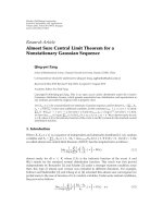
5.2. Results
Results in Figures 2–4 are provided for a 3-user (3,1) system
with the CSI uncertainty parameters U
(m)
T
= I, ξ
(m)
T

= ξ,
for all m. In Figures 2 and 3, the users’ target SINR are
set to be 5 (dB) while 10 (dB) is considered in Figure 4.
Results in the first two figures examine the performance
17
16
15
14
13
12
11
10
9
Output SINR of user 1 (dB)
00.05 0.10.15 0.20.25 0.30.35
CSIT error bound ξ
T
Target SINR
Optimal power-only allocation (14) with ZF
Proposed algorithm/optimal solution
Nonrobust design
Figure 4: The user’s output SINR averaged over channel uncer-
tainty for a given channel realization for various channel error
bound for a 3-user (3,1) system with γ
= 10 (dB).
of various schemes with small channel uncertainty bound,
up to ξ
= 0.1. Results in Figure 2 show the output SINRs
of user 1 for a particular channel realization, averaged
over the channel uncertainty. As we can see, the proposed

algorithm (which is optimal for MISO) and the optimal
power-only allocation achieve slightly greater SINR than
the target, which is expected because the optimization is
done in a way that the target can still be achieved at the
worst error conditions. In addition, results also illustrate
that the lower bounding approach achieves much higher
SINR than required and this loose bound leads to a huge
power penalty for ensuring the required QoS. In particular,
results in Figure 3 show that the SNR penalty of the SINR
bounding approach (18) grows with the channel error bound
and there is an SNR gap of as large as 10 (dB) if ξ
= 0.1, as
compared to the proposed algorithm and the optimal power-
only allocation. Moreover, results indicate that the optimal
joint power and beamforming solution performs similarly to
the optimal power-only allocation with fixed beamforming
vectors. However, we will soon observe that this is only the
case for systems with small number of users, and that the
channel is feasible for both solutions. From the transmit SNR
point of view, the nonrobust design is always the best but
a close observation of the data in Figure 2 reveals that the
output SINR is always smaller than the target, meaning that
the solution is actually not feasible. This problem becomes
much more apparent when γ
= 10 (dB) is considered in
Figure 4, and the gap between the output and target SINRs
grows farther apart as ξ increases.
In Figure 5, the feasibility regions of the optimal
solution, the optimal power-only allocation (19)with
ZF beamforming vectors, and the method using (18)are

12 EURASIP Journal on Advances in Signal Processing
Table 1: Service probabilities for a 2-user (2,1) system with imperfect CSIT but perfect CSIR.
Channel error bound ξ
Proposed
algorithm
(Section 4.3)
Optimal power
(19) with fixed ZF
vectors
(Section 3.3.3)
Solution using
lower bound (18)
(Section 3.2)
Nonrobust design
0.01
110.82
0.24
0.05
0.98 0.97 0.17
0.22
0.1
0.9 0.87 0.001
0.20
0.15
0.78 0.71 0
0.17
0.2
0.65 0.55 0
0.15
0.3

0.32 0.22 0
0.04
plotted for a particular channel realization

h
1
= [1.2272 +
0.4176i 0.1014
−0.3508i
],

h
2
= [−0.8694 + 1.2169i
0.2530
−1.1055i] of a 2-user (2,1) system.(Note that as these
three problems are all convex, they can be optimally solved
and the feasibility can also be easily checked using some
standard numerical algorithms for convex optimization,
such as the interior-point method.) In this figure, γ
= 5
(dB) and ξ
= 0.05 are assumed. The vertices indicate the
minimum transmit power (or SNR) needed for each scheme.
As we can see, the region for the lower bounding approach
is the smallest while the region for the optimal solution is
the largest and embraces that of the other two schemes. This
demonstrates that although previous results have shown that
the optimal solution and the optimal power-only allocation
perform similarly, there is a detrimental implication on

the feasibility by not optimizing the beamforming vectors
and the power allocation jointly. This point will further be
elucidated later in Table 1.
Results have so far shown that for multiuser MISO
systems, the proposed algorithm performs similarly as the
power-only optimization with ZF beamforming vectors. This
conclusion is however not true for a MIMO system and when
the channel uncertainty is more severe, for example, ξ as
large as 0.3. These results are shown in Figure 6 for 3-user
(3,2) and 4-user (4,3) systems with γ
= 10 (dB). As we can
see, larger gaps in SNR are observed and they grow consider-
ably with the channel error bound ξ and the number of users.
In particular, a gap of 8 (dB) is observed for a 4-user system
when ξ
= 0.3 while a gap of 7 (dB) appears for a 3-user
system with the same level of CSIT uncertainty. Note that the
results in this figure are for the cases with both perfect and
imperfect CSIR since the transmit SNR depends only on the
transmit beamforming vectors, obtained based on CSIT.
The performances of various algorithms when they are
all feasible are pretty well addressed now. However, it is
also important to know how they actually perform for
general random channels and error conditions particularly
in terms of their service probability (i.e., the probability that
a given method gives a feasible solution with the users’ SINR
constraints satisfied). Here, we examine this by providing
the service (or nonoutage) probabilities for the various algo-
rithms in Tables 1 and 2. Results in the tables illustrate that
the proposed algorithm decreases the probability of outage

14
12
10
8
6
4
2
0
−2
Transmit SNR of user 2 (dB)
02468101214
Transmit SNR of user 1 ( dB)
Optimal region
Robust solution using
lower bound (13)
Optimal power-only
allocation (14) with ZF
Figure 5: The feasibility regions of a 2-user (2,1) system for various
robust algorithms for a particular channel realization.
24
22
20
18
16
14
12
10
8
Total transmit SNR (dB)
0.10.15 0.20.25 0.3

Channel error bound ξ
T
Optimal power-only allocation (28) with ZF, 3-user (3, 2)
Proposed algorithm, 4-user (4, 3)
Proposed algorithm, 3-user (3, 2)
Optimal power-only allocation (28) with ZF, 4-user (4, 3)
Figure 6: The total transmit SNR versus the channel error bound
for 3-user (3,2) and 4-user (4,3) systems.
Gan Zheng et al. 13
Table 2: Service probabilities for multiuser MIMO systems where both imperfect CSIT and imperfect CSIR are considered such that ξ
(m)
T
= ξ
for all m, ξ
(m)
R
= ξ

for all m and ξ = 2ξ

.
Channel error Robust 2-user Nonrobust 2-user Robust 3-user Nonrobust 3-user Robust 4-user Nonrobust 4-user
bound ξ (2,2) (2,2) (3,2) (3,2) (4,3) (4,3)
0.01 1 0.25 1 0.12 1 0.061
0.05 1 0.23 1 0.1 1 0.049
0.1 1 0.21 0.99 0.085 1 0.035
0.15 0.99 0.19 0.99 0.066 0.99 0.03
0.2 0.98 0.18 0.98 0.053 0.99 0.02
0.3 0.84 0.14 0.77 0.034 0.98 0.01
Table 3: The probability, P , that the proposed algorithm (22) does not give an all-rank-1 solution. In this table, ∗ means that (22)doesnot

even have a feasible solution.
3-user (3,1) system Ellipsoid Nonellipsoid
Ranks of (U
(1)
T
, U
(2)
T
, U
(3)
T
) (3, 3, 3) (3, 3, 2) (3, 2, 2) (3, 1, 1)
P 0.0226 1 1
∗
4-user (4,1) system Ellipsoid Nonellipsoid
Ranks of (U
(1)
T
, U
(2)
T
, U
(3)
T
, U
(4)
T
) (4, 4, 4, 4) (4, 3, 3, 2) (4, 3, 2, 1) (4, 2, 1, 1)
P 0.0274 1 1
∗

5-user (5,1) system Ellipsoid Nonellipsoid
Ranks of (U
(1)
T
, U
(2)
T
, U
(3)
T
, U
(4)
T
) (5, 5, 5, 5, 5) (5, 4, 4, 3, 2) (5, 4, 3, 3, 2) (5, 4, 3, 2, 1)
P 0.0296 1 1
∗
by orders of magnitude, when compared to the nonrobust
design. Besides, there is a remarkable increase in the service
probability by using the proposed algorithm over the optimal
power-only allocation. On the other hand, however, if ξ
is too large, the problem itself is more likely to become
infeasible (and there exists no robust solution), leading to an
unacceptably low service probability. In addition, we can see
that for a given channel error bound ξ, multiuser MIMO has
a much higher service probability than multiuser MISO even
if imperfect CSIR is considered for the MIMO cases.
In Ta ble 3 , the tightness of the relaxation approach is
examined and the probability that the proposed algorithm
(22) does not give an all-rank-1 solution is shown, which is
designated as P . In the simulations, ξ

= 0.1 and random
SINR requirements are considered. The results are obtained
by averaging over 10
5
independent channel realizations and
{U
(m)
T
}. It is observed that with full-rank matrices {U
(m)
T
}
(i.e., the CSI error regions are ellipsoids), the rank-1 solution
exists with high probability, while with nonfull-rank
{U
(m)
T
}
(i.e., nonellipsoids), the proposed algorithm always outputs
a higher-rank solution and in some cases, the problem (22)
is even infeasible.
6. CONCLUSION
This paper has studied the worst-case robust beamforming
design of a downlink multiuser MIMO antenna system
where the CSIT and CSIR are known but imperfect, and
the channel uncertainty regions, which are modeled by
ellipsoids, are also known. With an aim to minimizing
the overall transmit power while ensuring that the users’
target SINRs for all possible channel uncertainty conditions
within the ellipsoids, this paper has presented techniques

to jointly optimize the power allocation and the transmit-
receive beamforming vectors for the users, based on the
imperfect CSIT, the perfect or imperfect CSIR, and the
channel uncertainty regions. Using S-procedure and rank
relaxation, it is possible to obtain the globally optimal joint
robust power and beamforming solution for a multiuser
MISO system while a convergent iterative algorithm has
been proposed to obtain a suboptimal robust solution for
a multiuser MIMO system. Simulation results have demon-
strated that the proposed algorithm yields a significant power
reduction to ensure robustness than an SINR bounding
approach, and the optimal power-only allocation with fixed
ZF beamforming vectors. The proposed algorithm has also
been shown to have the largest feasibility region and yield
the least outage probability as compared to other robust and
nonrobust schemes.
APPENDIX
A. DERIVATION OF THE KARUSH-KUHN-TUCKER
(KKT) CONDITIONS FOR PROBLEM (22)
Introducing the dual variables for all m,
λ
m
, r
(m)
T
, r
(m)
R
≥ 0,
W

m

⎡
⎣
λ
m
v
†
m
v
m
V
m
⎤
⎦
, S
m
 0,
(A.1)
14 EURASIP Journal on Advances in Signal Processing
the Lagrangian of (22)isgivenby
L(
{T
m
}, s
(m)
T
, s
(m)
R

, S
m
, r
(m)
T
, r
(m)
R
, W
m
)
=
M

m=1
[trace (T
m
) −trace (T
m
S
m
)] −
M

m=1
(r
(m)
T
s
(m)

T
+ r
(m)
R
s
(m)
R
)
−
M

m=1
trace
⎛
⎝
⎡
⎣
K

h
m
Q
m
Q
m

h
†
m
Q

m
+ s
(m)
T
U
(m)
T
⎤
⎦
W
m
⎞
⎠
,
(A.2)
where K denotes

h
m
Q
m

h
†
m
−γ
m
N
0
−s

(m)
T
ξ
(m)
T
2
.
Using the first-order optimality conditions
∂L
∂s
(m)
T
=−r
(m)
T
+ λ
m
ξ
(m)
T
2
−trace (U
(m)
T
V
m
) = 0,
∂L
∂s
(m)

R
=−r
(m)
R
+ λ
m
ξ
(m)
R
2
−trace (U
(m)
R
V
m
) = 0,
∂L
∂T
m
= I −S
m
−(λ
m

h
†
m

h
m

+ v
m

h
m
+

h
†
m
v
†
m
+ V
m
)
+
M

n=1
n
/
=m
γ
n
(λ
n

h
†

n

h
n
+ v
n

h
n
+

h
†
n
v
†
n
+ V
n
) = 0,
(A.3)
we can obtain the following dual problem
max
{λ
m
,V
m
,v
m
}

M
m
=1
M

m=1
λ
m
γ
m
N
0
s.t.
⎧
⎪
⎪
⎪
⎪
⎪
⎪
⎪
⎪
⎪
⎪
⎪
⎪
⎪
⎪
⎪
⎪

⎨
⎪
⎪
⎪
⎪
⎪
⎪
⎪
⎪
⎪
⎪
⎪
⎪
⎪
⎪
⎪
⎪
⎩
λ
m
ξ
(m)
T
2
−trace (U
(m)
T
V
m
) ≥ 0,

λ
m
ξ
(m)
R
2
−trace (U
(m)
R
V
m
) ≥ 0,
I
−(λ
m

h
†
m

h
m
+ v
m

h
m
+

h

†
m
v
†
m
+ V
m
)
+
M

n=1
n
/
=m
γ
n
(λ
n

h
†
n

h
n
+ v
n

h

n
+

h
†
n
v
†
n
+ V
n
)  0
⎡
⎣
λ
m
v
†
m
v
m
V
m
⎤
⎦

0.
(A.4)
ACKNOWLEDGMENTS
This work was supported in part by The Hong Kong Research

Grants Council under Grant HKU7175/03E and The Uni-
versity Research Committee of The University of Hong
Kong, and in part by The Engineering and Physical Science
Research Council (EPSRC) under Grant EP/D058716/1.
REFERENCES
[1]T.S.Rappaport,Wireless Communications: Principles and
Practice, Prentice Hall, Upper Saddle River, NJ, USA, 1996.
[2] G. J. Foschini and M. J. Gans, “On limits of wireless com-
munications in a fading environment when using multiple
antennas,” Wireless Personal Communications,vol.6,no.3,pp.
311–335, 1998.
[3] I. E. Telatar, “Capacity of multi-antenna Gaussian channels,”
Tech. Rep., AT & T Bell Labs, Murray Hill, NJ, USA, 1995.
[4] V. Tarokh, N. Seshadri, and A. R. Calderbank, “Space-time
codes for high data rate wireless communication: performance
criterion and code construction,” IEEE Transactions on Infor-
mation Theory, vol. 44, no. 2, pp. 744–765, 1998.
[5] A. Goldsmith, S. A. Jafar, N. Jindal, and S. Vishwanath,
“Capacity limits of MIMO channels,” IEEE Journal on Selected
Areas in Communications, vol. 21, no. 5, pp. 684–702, 2003.
[6] S. M. Alamouti, “A simple transmit diversity technique for
wireless communications,” IEEE Journal on Selected Areas in
Communications, vol. 16, no. 8, pp. 1451–1458, 1998.
[7] G. G. Raleigh and J. M. Cioffi, “Spatio-temporal coding for
wireless communication,” IEEE Transactions on Communica-
tions, vol. 46, no. 3, pp. 357–366, 1998.
[8] K K. Wong, R. S. K. Cheng, K. Ben Letaief, and R. D. Murch,
“Adaptive antennas at the mobile and base stations in an
OFDM/TDMA system,” IEEE Transactions on Communica-
tions, vol. 49, no. 1, pp. 195–206, 2001.

[9] M. Costa, “Writing on dirty paper,” IEEE Transactions on
Information Theory, vol. 29, no. 3, pp. 439–441, 1983.
[10] H. Weingarten, Y. Steinberg, and S. Shamai, “The capacity
region of the Gaussian multiple-input multiple-output broad-
cast channel,” IEEE Transactions on Information Theory, vol.
52, no. 9, pp. 3936–3964, 2006.
[11] S. Vishwanath, N. Jindal, and A. Goldsmith, “Duality,
achievable rates, and sum-rate capacity of Gaussian MIMO
broadcast channels,” IEEE Transactions on Information Theory,
vol. 49, no. 10, pp. 2658–2668, 2003.
[12] W. Yu and J. M. Cioffi, “Sum capacity of Gaussian vector
broadcast channels,” IEEE Transactions on Information Theory,
vol. 50, no. 9, pp. 1875–1892, 2004.
[13] F. Rashid-Farrokhi, K. J. R. Liu, and L. Tassiulas, “Transmit
beamforming and power control for cellular wireless systems,”
IEEE Journal on Selected Areas in Communications, vol. 16, no.
8, pp. 1437–1450, 1998.
[14] M. Bengtsson and B. Ottersten, “Optimal and suboptimal
transmit beamforming,” in Handbook of Antennas in Wireless
Communications, CRC Press, Boca Raton, Fla, USA, 2001.
[15] K K. Wong, R. D. Murch, and K. B. Letaief, “Performance
enhancement of multiuser MIMO wireless communication
systems,” IEEE Transactions on Communications, vol. 50, no.
12, pp. 1960–1970, 2002.
[16] Z. Pan, K K. Wong, and T S. Ng, “Generalized multiuser
orthogonal space-division multiplexing,” IEEE Transactions on
Wireless Communications, vol. 3, no. 6, pp. 1969–1973, 2004.
[17] G. Zheng, K K. Wong, and T S. Ng, “Convergence analysis
of downlink MIMO antenna systems using second-order cone
programming,” in Proceedings of the 62nd IEEE Vehicular

Technology Conference (VTC ’05), vol. 1, pp. 492–496, Dallas,
Tex, USA, September 2005.
[18] M. Schubert and H. Boche, “Solution of the multiuser down-
link beamforming problem with individual SINR constraints,”
IEEE Transactions on Vehicular Technology,vol.53,no.1,pp.
18–28, 2004.
[19] A. Wiesel, Y. C. Eldar, and S. Shamai, “Linear precoding
via conic optimization for fixed MIMO receivers,” IEEE
Transactions on Signal Processing, vol. 54, no. 1, pp. 161–176,
2006.
[20] J. Diaz, Z. Latinovic, and Y. Bar-Ness, “Impact of imperfect
channel state information upon the outage capacity of rayleigh
fading channels,” in Proceedings of IEEE Global Telecommu-
nications Conference (GLOBECOM ’04), vol. 2, pp. 887–892,
Dallas, Tex, USA, November-December 2004.
Gan Zheng et al. 15
[21] T. Yoo and A. Goldsmith, “Capacity and power allocation for
fading MIMO channels with channel estimation error,” IEEE
Transactions on Information Theory, vol. 52, no. 5, pp. 2203–
2214, 2006.
[22] A. Vakili, M. Sharif, and B. Hassibi, “The effect of channel
estimation error on the throughput of broadcast channels,”
in Proceedings of IEEE International Conference on Acoustics,
Speech and Signal Processing (ICASSP ’06), vol. 4, pp. 29–32,
Toulouse, France, May 2006.
[23] N. Jindal, “MIMO broadcast channels with finite-rate feed-
back,” IEEE Transactions on Information Theory, vol. 52, no.
11, pp. 5045–5060, 2006.
[24] H. Cox, R. M. Zeskind, and M. M. Owen, “Robust adaptive
beamforming,” IEEE Transactions on Signal Processing, vol. 35,

no. 10, pp. 1365–1376, 1987.
[25] K. L. Bell, Y. Ephraim, and H. L. Van Trees, “A Bayesian
approach to robust adaptive beamforming,” IEEE Transactions
on Signal Processing, vol. 48, no. 2, pp. 386–398, 2000.
[26] D. P. Palomar, A unified framework for communicat i ons through
MIMO channels, Ph.D. dissertation, Technical University of
Catalonia, Barcelona, Spain, May 2003.
[27]A.Pascual-Iserte,D.P.Palomar,A.I.P
´
erez-Neira, and
M.
´
A. Lagunas, “A robust maximin approach for MIMO
communications with imperfect channel state information
based on convex optimization,” IEEE Transactions on Signal
Processing, vol. 54, no. 1, pp. 346–360, 2006.
[28] A. Wiesel, Y. C. Eldar, and S. Shamai, “Optimization of the
MIMO compound capacity,” IEEE Transactions on Wireless
Communications, vol. 6, no. 3, pp. 1094–1101, 2007.
[29] J. Wolfowitz, Coding Theorems of Information Theory,
Springer, Berlin, Germany, 3rd edition, 1978.
[30] S. A. Vorobyov, A. B. Gershman, and Z Q. Luo, “Robust
adaptive beamforming using worst-case performance opti-
mization: a solution to the signal mismatch problem,” IEEE
Transactions on Signal Processing, vol. 51, no. 2, pp. 313–324,
2003.
[31] M. Biguesh, S. Shahbazpanahi, and A. B. Gershman,
“Robust downlink power control in wireless cellular systems,”
EURASIP Journal on Wireless Communications and Network-
ing, vol. 2004, no. 2, pp. 261–272, 2004.

[32] M. Payar
´
o, Impact of channel state information on the analysis
and design of multiantenna communicationv systems,Ph.D.
dissertation, Technical University of Catalonia, Barcelona,
Spain, February 2007.
[33] M. Payar
´
o, A. Pascual-Iserte, and M.
´
A. Lagunas, “Robust
power allocation designs for multiuser and multiantenna
downlink communication systems through convex optimiza-
tion,” IEEE Journal on Selected Areas in Communications, vol.
25, no. 7, pp. 1390–1401, 2007.
[34] M. B. Shenouda and T. N. Davidson, “Linear matrix inequal-
ity formulations of robust QoS precoding for broadcast
channels,” in Proceedings of the Canadian Conference on
Electrical and Computer Engineering (CCECE ’07), pp. 324–
328, Vancouver, Canada, April 2007.
[35] M. B. Shenouda and T. N. Davidson, “Convex conic formu-
lations of robust downlink precoder designs with quality of
service constraints,” IEEE Journal on Selected Topics in Signal
Processing, vol. 1, no. 4, pp. 714–724, 2007.
[36] A. L. Fradkov and V. A. Yakubovich, “The S-procedure and the
duality relation in convex quadratic programming problems,”
Vestnik Leningrad University: Mathematics, vol. 155, no. 1, pp.
81–87, 1973.
[37] S. Boyd and L. Vandenberghe, Convex Optimization
,Cam-

bridge University Press, Cambridge, UK, 2004.
[38] W. Rhee, W. Yu, and J. Cioffi, “The optimality of beamforming
in uplink multiuser wireless systems,” IEEE Transactions on
Wireless Communications, vol. 3, no. 1, pp. 86–96, 2004.
[39] T. Yoo and A. Goldsmith, “On the optimality of multiantenna
broadcast scheduling using zero-forcing beamforming,” IEEE
Journal on Selected Areas in Communications,vol.24,no.3,pp.
528–541, 2006.
[40] A. Bayesteh and A. K. Khandani, “On the user selection for
MIMO broadcast channels,” in Proceedings of IEEE Interna-
tional Symposium on Information Theory (ISIT ’05), pp. 2325–
2329, Adelaide, Australia, September 2005.
[41] F. Boccardi and H. Huang, “A near-optimum technique
using linear precoding for the MIMO broadcast channel,”
in Proceedings of IEEE International Conference on Acoustics,
Speech and Signal Processing (ICASSP ’07), vol. 3, pp. 17–20,
Honolulu, Hawaii, USA, April 2007.
[42] D. Bertsimas and M. Sim, “Tractable approximations to robust
conic optimization problems,” Mathematical Programming,
vol. 107, no. 1-2, pp. 5–36, 2006.
[43] I. P
´
olik and T. Terlaky, “A survey of the S-lemma,” SIAM
Review, vol. 49, no. 3, pp. 371–418, 2007.
[44] A. Ben-Tal and A. S. Nemirovskii, Lectures on Modern Convex
Optimization, Society for Industrial and Applied Mathematics,
Philadelphia, Pa, USA, 2001.
[45] A. Beck and Y. C. Eldar, “Strong duality in nonconvex
quadratic optimization with two quadratic constraints,” SIAM
Journal on Optimization, vol. 17, no. 3, pp. 844–860, 2006.

[46] R. A. Monzingo and T. W. Miller, Introduction to Adaptive
Arrays, John Wiley & Sons, New York, NY, USA, 1980.