Báo cáo hóa học: " Research Article A Wireless Sensor Network for RF-Based Indoor Localization" pptx

Hindawi Publishing Corporation
EURASIP Journal on Advances in Signal Processing
Volume 2008, Article ID 731835, 27 pages
doi:10.1155/2008/731835
Research Article
A Wireless Sensor Network for RF-Based Indoor Localization
Ville A. Kaseva,
1
Mikko Kohvakka,
1
Mauri Kuorilehto,
2
Marko H
¨
annik
¨
ainen,
1
and Timo D. H
¨
am
¨
al
¨
ainen
1
1
Department of Computer Systems, Tampere University of Technology, P.O. Box 553, 33101 Tampere, Finland
2
Nokia, Devices R&D, Visiokatu 3, 33720 Tampere, Finland
Correspondence should be addressed to Ville A. Kaseva, ville.a.kaseva@tut.fi

Received 14 August 2007; Revised 11 January 2008; Accepted 26 March 2008
Recommended by Davide Dardari
An RF-based indoor localization design targeted for wireless sensor networks (WSNs) is presented. The energy-efficiency of mobile
location nodes is maximized by a localization medium access control (LocMAC) protocol. For location estimation, a location
resolver algorithm is introduced. It enables localization with very scarce energy and processing resources, and the utilization of
simple and low-cost radio transceiver HardWare (HW) without received signal strength indicator (RSSI) support. For achieving
high energy-efficiency and minimizing resource usage, LocMAC is tightly cross-layer designed with the location resolver algorithm.
The presented solution is fully calibration-free and can cope with coarse grained and unreliable ranging measurements. We analyze
LocMAC power consumption and show that it outperforms current state-of-the-art WSN medium access control (MAC) protocols
in location node energy-efficiency. The feasibility of the proposed localization scheme is validated by experimental measurements
using real resource constrained WSN node prototypes. The prototype network reaches accuracies ranging from 1 m to 7 m.With
one anchor node per a typical office room, the current room of the localized node is determined with 89.7% precision.
Copyright © 2008 Ville A. Kaseva et al. This is an open access article distributed under the Creative Commons Attribution License,
which permits unrestricted use, distribution, and reproduction in any medium, provided the original work is properly cited.
1. INTRODUCTION
The problem of localization includes determining where
a given node is physically located [1]. The existence of
location information enables a myriad of functions. At appli-
cation level, activities such as location and asset tracking,
monitoring, context aware applications [2], and personal
positioning [3] are made possible. Enabled protocol-level
functions include location-based routing [4, 5], and geo-
graphic addressing [6].
The Global Positioning System (GPS) [7] is a commonly
used technology for localization. However, GPS performs
poorly in indoor environments. Localization using wireless
local area networks (WLANs) has been widely studied as
a potential solution for feasible indoor localization [8–16].
However, the application space of both GPS and WLAN
localization is limited due to practical considerations such

as the size, form factor, cost, and relatively large power
consumption of the nodes.
Wireless sensor networks (WSNs) form a potential
technology for ubiquitous indoor localization due to their
autonomous nature, low power consumption [17], and small
size factor [18]. The existence of WSNs is enabled by the
recent advances in wireless communications and electronics
[19]. A WSN may consist of a very large number of small
sensor nodes [17], which gather information from their
environment by various sensors, process the collected infor-
mation, control actuators, and communicate wirelessly with
each other. Due to the very large number of nodes, frequent
battery replacements and manual network configuration are
inconvenient or even impossible. Thus, the networks must
be self-configuring and self-healing, and the nodes must
operate with small batteries for a lifetime of months to
years [17, 20]. This results in very scarce energy budget and
constrained data processing, memory, and communication
resources.
The usage of the radio transceiver as localization Hard-
Ware (HW) is an attractive choice due to its dual-use
possibility and inherent existence in WSN nodes. Typically,
localization can be performed by measuring signal strengths
from the transmissions of neighbors. However, the most low-
cost and low-power radio transceivers do not include such a
possibility.
Low-power ad hoc medium access control (MAC) proto-
cols have come into existence upon the emergence of WSNs.
A radio transceiver is the most power consuming component
2 EURASIP Journal on Advances in Signal Processing

in a WSN node [21]. WSN MAC protocols achieving the
lowest power consumption minimize radio usage by accu-
rately synchronizing transmissions and receptions with their
neighbors. Typically, the protocols are designed for relatively
static network environment, and the energy-efficiency of
mobile nodes is degraded. This is problematic in localization
point of view, since many located objects can be mobile.
As nodes are moving, their network neighborhood
changes introducing increased amount of neighbor dis-
covery attempts. In current WSN MAC proposals, the
neighbor discoveries are typically performed by energy-
hungry network scans requiring relatively long channel
receptions. Energy-efficient neighbor discovery protocol
(ENDP) [21] introduces a feasible and low-power solution
for neighbor discovery. However, also ENDP necessitates a
network scan at a start-up and when all communication
links to neighbors are broken. The situation is difficult,
when a node moves away from the range of other nodes
resulting in frequent network scanning. Moreover, to achieve
the best possible localization accuracy, mobile nodes need
to update measurements frequently from as many neigh-
bors as possible. In current protocols, this necessitates
frequent channel reception at the cost of high energy
consumption.
Our design aims to achieve ubiquitous real-time localiza-
tion with low-cost resource constrained nodes. The location
nodes are localized using single-hop ranging measurements.
The localization data is forwarded via a multihop anchor
node network. The presented design builds on top of
following objectives and requirements.

(i) Location node energy-efficiency. To enable ubiquitous
localization, the location nodes need to run unat-
tended for years with small batteries. Thus, they
should reach high energy-efficiency. Anchor nodes
are static and considered to be energy unconstrained.
Such an assumption is valid, for example, in the
field of infrastructure WSNs [22]. Practically, this
means that the anchor nodes are mains-powered or
equipped with large enough batteries. Location nodes
can be highly mobile or relatively static. In either
case, the one-hop anchor node neighbors should
be reached without considerable increase in power
consumption. In addition, a location node can be
removed from the anchor network coverage area for
undetermined time periods. This should not result
in actions reducing energy-efficiency. Addressing the
above concerns necessitates the minimization of
location node radio usage and MCU active time.
Also, energy-inefficient neighbor discoveries should
be mitigated.
(ii) Scalability. High densities of location nodes can
coexist in the same physical area. Thus, recognizing
congestion and adapting to it is an essential demand
for the utilized MAC. The spatial scalability of a
localization network is highly dependent on the capa-
bilities of the used protocols. In addition, practical
issues such as ease of deployment and device costs are
in central position.
(iii) Bidirectional communication between location nodes
and anchor nodes. The ability to communicate with

location nodes enables protocol cooperation and
expands application-level design space significantly.
At communication protocol level, distributed algo-
rithms such as data aggregation, fusion, and coop-
erative localization are made possible. Application-
level issues include, for example, monitoring and user
interaction. A location node may integrate sensors
with which it can monitor its environment and/or
the object or person it is attached to. Furthermore,
a person with a location node may send predefined
messages and read status information by using a
simple user interface (UI) provided by the loca-
tion node or a device connected to the location
node. Applications requiring reliable communication
should be taken into account when designing the data
transfer support.
(iv) Hardware constraints. For feasible implementation
on low-cost, and thus, resource constrained HW
platforms, the used protocols should strive for low
complexity. Low-cost radio transceivers may not
include received signal strength indicator (RSSI),
but usually the selection of different transmission
power levels is possible. Limited HW capabilities lead
to limited ranging information, which the location
estimation algorithm has to tolerate.
(v) Accuracy. Our goal is not to improve upon the accu-
racy of the related RF-based localization approaches,
but rather to achieve similar results with very low
energy consumption and complexity of nodes. Due
to the inaccuracy of the used ranging method we

have targeted to the scale of few meters and to good
precision in room-level accuracy.
(vi) Real-time operation.Inorderforlocationdatatobe
useful, it usually needs to be obtained in real-time.
Real-time operation requires low data forwarding
latencies from the localized objects to the place of
exploitation.
To address the aforementioned objectives and require-
ments, we present
(i) a novel MAC protocol, called localization MAC
(LocMAC), which enables highly energy-efficient
location nodes and low-latency multihop data relay,
and
(ii) a novel lightweight location resolver algorithm capa-
ble of estimating locations using coarse grained and
unreliable RF transmission power measurements.
For achieving high energy-efficiency and minimizing re-
source usage, LocMAC is tightly cross-layer designed with
the location resolver algorithm. It includes a built-in support
for energy-efficient RSSI-free ranging. The location nodes
are relieved from doing neighbor discoveries by an asym-
metric protocol approach. The location resolver algorithm
employs a novel learning-based transmission power to
VilleA.Kasevaetal. 3
Location
resolver
Location
database
Server
Data relay

GUI
Ranging
measurement
data
Single-hop ranging measurements
Location node
Anchor node
Gateway anchor node
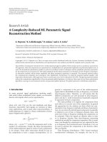
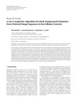
Figure 1: Centralized localization network architecture.
distance mapping technique. The scheme is fully calibration
free making ad hoc deployment feasible.
The operation of LocMAC is verified by analytical
performance analysis, comparison with low-power WSN
MAC proposals, and simulations. The feasibility of the
proposed localization scheme is validated by experimental
measurements using real WSN prototypes. A centralized
approach depicted in Figure 1 is utilized. However, cen-
tralized operation is not a fundamental constraint to our
scheme. Thus, we will also briefly discuss the minor changes
needed to make the proposed solution distributed and
cooperative.
Thekeycontributionsofthispaperare
(i) the design of LocMAC and the location resolver
algorithm,
(ii) comparison against current state-of-the-art low-
power MAC protocols and RF-based indoor localiza-
tion proposals, and
(iii) experiments with real resource constrained WSN
prototypes.
The rest of the paper is organized as follows. In Section 2,

we survey related indoor localization approaches, low-
power WSN MAC protocols, and WSN MAC mobility sup-
port. Section 3 describes the LocMAC design. The location
resolver algorithm is presented in Section 4.InSection 5,
LocMAC is analyzed mathematically and with simulations.
Furthermore, LocMAC is compared against state-of-the-art
WSN MAC proposals. In Section 6, prototype implemen-
tation, experiments, and results are presented. A compar-
ison against related localization proposals is presented in
Section 7. Section 8 discusses localization decentralization
and optimization issues, and outlines our future work.
Finally, Section 9 concludes the paper.
2. RELATED RESEARCH
Ubiquitous localization has been widely studied during the
recent years. In general, the solutions focus on finding
effective location estimation algorithms and measurements
that correlate with location. In these designs, medium access
has either low priority or it is not considered at all. A detailed
survey on ubiquitous localization approaches and taxonomy
is given by Hightower and Borriello in [23].
The emergence of WSNs has generated a large amount
of MAC protocols aiming for energy- and resource-efficient
operation. Their design principles incorporated with local-
ization data acquisition can enable a whole new set of
applications.
2.1. Ubiquitous indoor localization
Localization approaches can be categorized to range-based,
proximity-based, and scene analysis. The underlying tech-
nologies vary from pure RF-based, to UltraSound (US),
InfraRed (IR), and multimodal solutions.

Range-based approaches rely on estimating distances
between location nodes and anchor nodes. This process is
called ranging. Received signal strength (RSS) is a common
RF-based ranging technique. Distances estimated using RSS
can have large errors due to multipath signals and shadowing
caused by obstructions [24, 25]. The inherent unreliability
has to be addressed in the used localization algorithms.
In [26, 27] RSS is replaced with multiple varying power
level beacon transmissions. To reduce quantization error, the
amount of used transmission power levels is relatively large.
Several location estimation techniques can be used in
range-based localization. Utilized methods include trilater-
ation [27, 28], weighted center of gravity calculation [29],
and Kalman filtering [9]. Many mathematical optimization
methods, such as the steepest descent method [8], sum of
errors minimization [26], and minimum mean square error
(MMSE) method [30], have been used to solve range-based
location estimation problems.
Proximity-based approaches exploiting RF signals [1, 10,
11, 31] estimate locations from connectivity information.
Such solutions are also commonly referred to as range-free
in the literature. In WLANs, mobile devices are typically
connected to the access point (AP) they are closest to (in
signal-space). In the strongest base station method [10,
11],
the location of the node is estimated to be the same as
the location of the AP to which it is connected. In [1,
31], the unknown location is estimated using connectivity
information to several anchor nodes. Only a very coarse-
grained location can be estimated using the strongest base

station method. The solutions presented in [1, 31] better the
granularity to some degree. Nevertheless, in order to reach
small granularities the connectivity-based schemes require
a very dense grid of anchor nodes. Their strength is fairly
simple implementation and modest HW requirements.
Scene analysis consists of an offline learning phase and
an online localization phase. The offline phase includes
recording RSS values corresponding to different anchor
nodes as a function of the users location. The recorded
RSS values and the known locations of the anchor nodes
are used either to construct an RF-fingerprint database [11,
12, 32], or a probabilistic radio map [13–16, 33]. In the
online phase, the location node measures RSS values to
4 EURASIP Journal on Advances in Signal Processing
different anchor nodes. With RF-fingerprinting, the location
of the user is determined by finding the recorded reference
fingerprint values that are closest to the measured one (in
signal space). The unknown location is then estimated to be
the one paired with the closest reference fingerprint or in
the (weighted) centroid of k-nearest reference fingerprints.
Location estimation using a probabilistic radio map includes
finding the point(s) in the map that maximize the location
probability.
The applicability and scalability of scene analysis
approaches are greatly reduced by the time-consuming
collection and maintenance of the RF sample database.
Searching trough the sample database or radio map is com-
putationally intensive. The joint clustering (JC) technique
[15] uses location clustering to reduce the computational
cost of searching the radio map. It betters the scalability

of the searching algorithm to some extent. MoteTrack [32]
achieves similar effect by disseminating the RF-fingerprint
database to an WSN and decentralizing the localization
procedure.
The described RF-based approaches [1, 26–33]canbe
considered to utilize networks with WSN characteristics. Due
to the autonomous operation of WSNs, the anchor network
installation is easy. Used nodes are small and of low-cost
thus enabling a cost-effective solution for localization. Since
WSNs aim to maximize energy-efficiency, battery-operated
nodes hold the potential to achieve long lifetimes.
WLANs are utilized in [8–16]. They are becoming more
and more popular offering increased availability. Accord-
ingly, the strength of WLAN-based localization schemes lies
in their ability to leverage existing network infrastructure.
The costs are increased since every located object must be
equipped with a relatively expensive WLAN adapter. WLANs
are designed primarily to optimize throughput. Energy-
efficiency is a secondary objective leading to shortened node
lifetime.
In general, RF signal strength-based localization pos-
sesses fundamental limits due to the unreliability of the
measurements [14]. There is strong evidence that, at best,
accuracy in the scale of meters can be achieved regardless of
the used algorithm or approach [14].
US-based approaches, namely Active Bat [34]and
Cricket [35–37], use time-of-flight ranging and can achieve
high accuracies. However, anchor nodes need to be posi-
tioned and orientated carefully due to the directionality of
US and the requirement for Line-of-Sight (LoS) exposure.

A dense network of anchor nodes is needed due to the
LoS requirement, short range of US, and the fact that
typically ranging measurements to at least four anchor nodes
are needed. The addition of US transmitters and receivers
increases HW costs and reduces energy-efficiency compared
to purely RF-based solutions. Some schemes [34, 36]require
multiple US transmitters/receivers per one HW platform
further increasing the HW costs.
IR-based solutions, such as Active Badge [38, 39], are
based on inferring proximity. They can localize location
nodes inside the range of LoS IR transmissions. IR-based
schemes suffer errors in the presence of obstructions. Also,
differing light and ambient IR levels, caused by for example
fluorescent lighting or direct sunlight, produce difficulties
[23, 35]. The anchor network costs are high because a dense
matrix of IR sensors is needed in order to avoid dead spots.
In the presence of a myriad of location sensing tech-
niques, data fusion has become an attractive location
estimation method. It can combine measurements from
multiple sensors while managing measurement uncertainty.
In [40], Fox et al. survey Bayesian filtering techniques capable
of multisensor fusion. Probabilistic fusion methods require
relative large amounts of computation. Thus, in the presence
of resource constrained nodes, a centralized implementation
running in a more powerful base station is often the only
feasible choice. For example, in the localization stack [41],
the fusion layer is implemented in Java.
Our previous research [42] presents a transmission
power -based path loss metering method, that does not
require RSSI functionality. The work presented in this paper

extends the described method to node localization. Our
work differs from RSSI-free approaches [26, 27] in three
ways. First, our location estimation algorithm is much less
computationally intensive than the ones used in [26, 27].
Secondly, the coarse-grained nature of RSSI-free ranging
is accounted for instead of using the signal measurements
as traditional ranging measurements with possibly larger
quantization error. Third, our approach can cope with any
amount of transmission power levels. More importantly, the
transmission power level amount can be much lower than
with [26, 27]. In general, the current localization approaches
rely on existing communication protocols. This leads to
inefficient performance especially in mobile scenarios.
2.2. Low-power medium access
Next, we introduce the operation principles of low-power
WSN MAC protocols and survey key proposals in the area.
Since these protocols are usually designed for relatively static
networks, dynamics, especially mobility, can introduce sig-
nificant additional energy consumption to their operation.
The mobility support for WSN MAC protocols is covered in
the latter part of the section.
2.2.1. MAC protocols
WSN MAC energy-efficiency is achieved by duty-cycling,
which includes active periods for data exchanges and sleep
periods for energy conservation. WSN MAC protocols can
be divided into three categories: random-access, sched-
uled contention-access, and Time Division Multiple Access
(TDMA). The low duty-cycle random-access MAC proto-
cols, such as WiseMAC [22, 43], B-MAC [44], SpeckMAC
[45], X-MAC [46], and SCP-MAC [47], are based on a

technique called low-power listening (LPL) (name preamble
sampling [48] is also used for a method identical to LPL).
It includes the procedure of periodically polling the wireless
channel to test for traffic. Typically, frames are transmitted
with a preceding preamble that is longer than the channel
poll interval. This ensures that the destination node is
awake during the actual data transmission. Low duty-cycle
random-access MAC protocols are relatively simple and
VilleA.Kasevaetal. 5
require less memory than scheduled contention-access and
TDMA-based low-duty cycle MACs [21]. Their energy-
efficiency is reduced due to high idle listening times (caused
by frequent channel sampling), and high overhearing. The
long preamble presents significant energy costs to the
transmission and reception of frames if not mitigated.
Scheduled contention-access low duty-cycle MAC proto-
cols, namely S-MAC [49], T-MAC [50], and IEEE 802.15.4
low-rate wireless personal area network (LR-WPAN) stan-
dard [51], utilize periodic active and sleep periods to achieve
duty-cycling. The start of the active period includes the
transmission of synchronization (SYNC) frames to commu-
nicate own schedule information to neighboring nodes. The
rest of the active period is reserved for data exchanges, which
typically use contention-access for medium arbitration.
TDMA-based low duty-cycle MAC protocols, including
SMACS [52], LEACH [53], PACT [54], TRAMA [55], SRSA
[56], and TUTWSN MAC [57], exchange data only in
predetermined synchronized time slots. Rest of the time
is spent in sleep mode. This makes the protocols virtually
collision-free and removes overhearing. The only sources

of idle listening are reception margins, which are usually
relatively small. In static networks, TDMA-based MAC
protocols can achieve even an order of a magnitude lower
energy consumption than low duty-cycle random-access and
scheduled contention-access MACs [45, 57].
2.2.2. Mobility support
As network dynamics increase, neighbor discovery starts
to produce significant energy overhead with synchronized
low duty-cycle MAC protocols, which include all scheduled
contention-access and TDMA-based protocols and SCP-
MAC from low duty-cycle random-access protocol family.
The rest of the low duty-cycle random-access protocols
are unsynchronized and do not require explicit neighbor
discovery.
Network scanning is the typical mechanism for neighbor
discovery in current low-power MAC proposals [21]. It may
consume energy equal to the transmission of thousands of
data packets [58].
The term network scanning refers to the generic pro-
cedure of continuous listening for neighbors’ control data
until sufficient knowledge of the neighborhood is obtained.
This requires the listening to go on for the duration of a
synchronization period. Thus, the term network scanning is
applicable to the following procedures:
(i) listening for in-channel signaling messages possibly
on one or many RF frequency channels, as in SCP-
MAC, S-MAC, T-MAC, and IEEE 802.15.4,
(ii) listening for out-of-channel signaling messages on a
network-wide fixed signaling channel, as in SMACS
and TUTWSN MAC, and

(iii) listening for signaling messages during a periodical
signaling period, as in LEACH, PACT, TRAMA, and
SRSA.
Several studies, such as [59, 60], address mobility and
the energy constraint at the network layer. However, work
aiming to improve energy-efficiency under mobility at the
MAC layer is more rare. Since majority of energy overhead
is caused by idle listening at the data link layer, significant
energy saving can be achieved by addressing mobility in the
MAC protocol [61].
Mobility-aware Sensor MAC (MS-MAC) [61]isbasedon
S-MAC. It adjusts network scan interval according to the
mobility of nodes. Mobility-adaptive MAC (MMAC) [62]
works similarly as MS-MAC, but it uses TRAMA as the basic
MAC protocol and adjusts the occurrence frequency of the
signaling period according to mobility. These approaches
allow mobile nodes to acquire new connections more
efficiently and reduce packet losses. However, the energy
consumption is high due to frequent networks scans.
Raviraj et al. [63] propose an adaptive frame size
predictor to overcome the energy-inefficiency caused by
frame losses in mobile scenarios. The approach can improve
energy-efficiency by using smaller frame sizes when the
wireless channel characteristics are poor. However, the
method does not consider neighbor discovery, and thus,
mitigates only the energy-inefficiency caused by larger bit
error rate due to mobility and Doppler shifts.
From the covered low duty-cycle MAC protocols, only
SMACS consider mobility explicitly. For mobile nodes, it
proposes an Eavesdrop-And-Register (EAR) algorithm. The

EAR algorithm is designed to save energy for stationary
nodes in the presence of mobile nodes. Mobile nodes
must listen almost constantly resulting in high energy
consumption. Thus, the algorithm is not applicable with
energy-constrained mobile nodes.
Our concurrent work, ENDP [21], reduces the need for
costly network scans by proactively distributing node sched-
ule information. Two-hop neighborhood synchronization
information is piggybacked in beacon transmissions. ENDP
can achieve low energy consumption when continuously
having at least one working link. At a start-up and when all
communication links to neighbors are broken, also ENDP
has to fall back on network scanning. To the best of our
knowledge, ENDP is currently the most energy-efficient
neighbor discovery protocol for dynamic WSNs using low
duty-cycle MAC protocols.
The work presented in this paper achieves energy-
efficient mobile location nodes by relieving them from doing
neighbor discoveries. For this, an asymmetric architecture,
where energy unconstrained anchor nodes listen almost
continuously, is used. The location node energy-efficiency is
independent of the scenario and environment.
3. LocMAC DESIGN
LocMAC is comprised of two subprotocols; LocMAC base
and LocMAC rela y. LocMAC base enables energy-efficient
single-hop localization data acquisition. It arbitrates the
wireless medium between location nodes. It can be inte-
grated to any data gathering network, whose operation
includes idle times. By giving the data gathering network
protocols higher priority and executing LocMAC base in

6 EURASIP Journal on Advances in Signal Processing
a separate channel, their operation is not affected. Thus,
LocMAC base does not dictate the usage of LocMAC relay.
LocMAC relay provides localization data aggregation and
low-latency data relay. It is primarily designed for multihop
data gathering using LocMAC base as the data source.
Thus, some parts of its functionality require the existence of
LocMAC base.
3.1. Energy-efficient localization data acquisition
LocMAC base enables energy-efficient location node opera-
tion. In the rest of this section, we will focus on its operation
principles.
3.1.1. Location node channel access and
collision avoidance
LocMAC base uses duty-cycling to achieve energy-efficiency.
Location node time is divided into active periods and
idle periods. A location node starts its active period by
transmitting N
lb
location beacons (LB), which constitute a
beacon set. Energy unconstrained anchor nodes use their
idle time listening for LBs in the location channel. They
acknowledge received LBs in a downlink slot following the
beacon set using a location beacon acknowledgement (LBA)
frame. Consecutive active and idle period constitutes a
beacon cycle, which is repeated at interval T
bc
. By making
anchor nodes scan for LBs, the location nodes are relieved
from performing active neighbor discovery.

The LBs are dual-purpose. First, they form the basis
of LocMAC base collision-avoidance (CA) mechanism with
the LBAs. Concurrently, LBs enable coarse-grained RSSI-free
RF-based ranging.
Only one downlink slot is used so that the energy
consumption and the time one location node occupies
the location channel would be minimal. The usage of one
downlink slot requires an arbitration mechanism in order to
avoid multiple anchor nodes transmitting in the same slot.
A reservation-based slot allocation mechanism is infeasible
because of high expected network dynamics and short-lived
links. Thus, simple randomization is used to control who is
allowed to transmit in the downlink slot.
LocMAC base divides time into discrete time slots
referred to as active period slots. Ideally, each active
period slot should contain the active period of only one
location node. Since location nodes access the channel
asynchronously, their active period slot boundaries do not
occur at same time instants. Thus, the active period slot
length is set to be two times as long as the active period
duration and the active period occurs at the middle of
the slot. This ensures that an active period occurring in a
randomly selected slot in the schedule of location node x can
collide with only one active period in the schedule of location
node y.
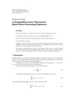
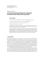
Figures 2 and 3 illustrate LocMAC base operation
principle. They present two location nodes, 11 and 12, and
two anchor nodes, 1 and 2. N
lb
is set to four. Transmission

powers are enumerated with integers from 1 to 4, 1 indicating
the lowest and 4 the highest transmission power. LB
n
denotes
Range with
the lowest
power beacon
Range with
the highest
power beacon
Anchor
node 1
Anchor
node 2
Location
node 12
Location
node 11
1
2
3
4
Figure 2: LocMAC base operation principle: relative locations of
anchor and location nodes and radio ranges with different trans-
mission powers.
a location beacon transmitted with power level n.Thenode
locations relative to each other and relative to radio ranges
are illustrated in Figure 2. In the depicted scenario, location
nodes infer overlapping active periods from two or more
missed LBAs. Due to space limitations in Figure 3, the active

period slot length is equal to the active period duration.
At epoch A in Figure 3,locationnode12isableto
successfully transmit LB
2
to anchor node 2 (no overlap
in time) and LB
4
to anchor node 1 (no overlap in radio
coverage). LB
3
of location node 11 collides with the downlink
slot of location node 12. Location node 11 still succeeds to
transmit LB
4
to both anchor nodes. However, the anchor
nodes omit acknowledging it, since they infer possible active
period overlap. Epoch B presents similar events as epoch A.
After epoch B, both location nodes have missed two LBAs.
Thus, the location nodes determine that they have conflicting
schedules. After inferring a conflicting schedule, a location
node chooses a new one by randomizing a new active period
slot.
The new active period slot is randomized between
interval [t
aps end(k)
, t
aps start(k+2)
], where t
aps end(k)
is the end

time of current active period slot (k)andt
aps start(k+2)
is the
start time of active period slot k + 2. The randomization
interval end is given by
t
aps start(k+2)
= t
aps end(k)
+2T
bc
−t
aps
,(1)
where T
bc
is the beacon cycle length and t
aps
is the active
period slot length. After a location node has randomized a
new slot, it adjusts its beacon cycle length to T
bc adj
for one
beacon cycle in order to adapt to the new schedule. After the
adaptation, the location node starts using the normal beacon
cyclelength(T
bc
) again.
Therandomizedslotindexcanbebetween[
−sidx,

sidx](sidx
∈ N
+
), where sidx = N
rnd slots
/2 − 1and
index 0 denotes a slot that would result in no adjustment
(i.e., T
bc adj
= T
bc
). N
rnd slots
denotes the amount of
randomization slots. Equal probability to temporarily adjust
beacon cycle shorter or longer results in
T
bc
= lim
n→∞

n
k
=0

t
bc(k+1)
−t
bc(k)


n
,(2)
VilleA.Kasevaetal. 7
Beacon set
No reception in
downlink slot
RX
TX
Location
node 12
RX
TX
Location
node 11
RX
TX
Anchor
node 2
RX
TX
Anchor
node 1
Collision
Active
period
Idle period T
bc adj
T
bc
Randomization slot

Successful reception
in downlink slot
No transmission in downlink slot Transmission in downlink slot Successful beacon reception
Idle listening
AB CD
−n −3 −2−10 1 2 3
n − 2
n
−1
n
−(n −1)
−(n −2)
Highest TX power beacon
Lowest TX power beacon
Figure 3: LocMAC base operation principle: LocMAC beacon cycle components, collision avoidance, and timing.
where t
bc(k)
is the start time of beacon cycle k. Thus, the
mean beacon cycle length is always T
bc
, which results in fair
channel access and predictable energy consumption.
In Figure 3 at the end of epoch B, location node 12
randomizes its active period to slot
−1 and location node
11 to slot 0 (sidx being n). At epoch C, the new schedules
are adopted, resulting in a collision-free situation. Now
both location nodes can successfully transmit their LBs and
receive corresponding LBAs. Location nodes continue with
same schedules at epoch D since they infer nonconflicting

situation from successful LBA receptions.
3.1.2. Detecting and handling false location beacons
A false LB reception occurs when an anchor node is situated
in the range of an LB transmitted with power P,butitcan
only hear LB(s) transmitted with power that is larger than P.
This situation can occur if
(i) an anchor starts listening the location channel in the
middle of an active period and/or
(ii) active periods of two or more location nodes overlap
partially.
Detecting falsely observed LBs has two benefits. First,
it serves as an indicator for partly overlapping, and thus,
conflicting active periods, as happens in Figure 3 at epochs
A and B. Secondly, the location estimation algorithm can be
informed of invalid input data.
When an anchor node starts listening the location
channel in the middle of an active period, a possibly false
LB can be detected by counting the time passed between the
listening start time (t
lst start
) and the reception time instant of
the LB (t
b
). The LB can be false if
t
b
−t
lst start
<t
bs

,(3)
where t
bs
is the beacon set length.
When active periods of two or more location nodes
overlap partially, a possibly false LB can be detected by
observing the time passed between the end of the last
detected active period (t
end ap
) and the reception time instant
of the current LB t
b
. Thus, an LB can be false if
t
b
−t
end ap
<t
bs
. (4)
3.1.3. Data transfer
LocMAC base enables low-rate data exchanges between lo-
cation nodes and anchor nodes. Both LBs and LBAs include
payload parts. Uplink data can be piggybagged in LB frames,
while downlink data can utilize LBA frames.
Two quality-of-service (QoS) classes, datagram and
reliable, are supported. Datagram protocol data units (PDU)
are transmitted once after which they are removed from the
PDU queue. Reliable PDUs remain in the queue until they
are acknowledged or an application-specific timeout occurs.

3.1.4. Scalability
The LB/LBA CA mechanism enables spatial scalability
by handling the hidden node problem [64] similarly to
CTS/RTS mechanism in IEEE 802.11 CSMA/CA [65]. Col-
lisions at the receiver (anchor node) are inferred from the
absence of acknowledgments (LBAs).
8 EURASIP Journal on Advances in Signal Processing
The active period slot randomization (APSR) mecha-
nism handles scalability in location node amount. The abso-
lute theoretical maximum amount (N
ln max
)ofcoexisting
location nodes in the same radio coverage area is given by
N
ln max
=

T
bc
t
aps

. (5)
When the location node amount in the same radio coverage
area starts to approach N
ln max
, the LocMAC base CA
performance will hinder due to congestion. Location nodes
adapt to congestion by increasing their beacon cycle lengths
(T

bc
), which in turn leads to increased N
ln max
.
In order to reduce interference range, an LBA frame
is always transmitted with the same transmission power as
the minimum received LB. By monitoring the received LBA
transmission powers, location nodes can gain information
about the amount of anchor nodes they can reach using a
certain transmission power. In the presence of excess anchor
nodes, the maximum LB transmission power can be scaled
down reducing the beacon set interference range. The down-
scaling of the transmission power results also in energy
savings, and shorter active period.
3.2. Low-latency data relay
LocMAC relay enables the anchor nodes to establish a
network for multihop data forwarding. It exploits both
TDMA and Frequency Division Multiple Access (FDMA) to
share the medium. The medium has to be arbitrated among
the relay nodes and between relay network and the location
nodes.
LocMAC relay specifies only the medium access. For
routing, for example a spanning tree algorithm resolving
minimum-hop routes to the sink can be used.
3.2.1. Network topology
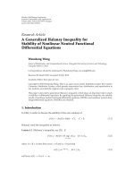
The LocMAC relay protocol exploits flat relay topology
superpositioned with a clustered data aggregation topology.
An example is illustrated in Figure 4. The relay network
consists of relay nodes and single or multiple sinks. The relay
nodes form a flat topology to enable data forwarding to the

sink(s). For data aggregation, clusters are established. Each
aggregation cluster consists of an aggregation cluster head
(ACH) and n subnodes acting as cluster members. At data
relay level relay nodes are homogenous.
The ACHs act as data aggregation points. Data aggrega-
tion is performed on measurements belonging to the same
beacon set. Location node ID and beacon set transmission
timestamp (either local or global time can be used for the
unique beacon set identifier formation) can be used to form
a unique identifier for measurements belonging to the same
beacon set. After the aggregation point, a flat topology is used
and subsequent data relaying and routing can be done by any
node in the relay network.
In Figure 4, the LBs transmitted by location node 1 are
heard by relay nodes 2, 3, and 4. Nodes 2 and 3 act as
subnodes. They forward LB information to their ACH, node
Aggregation hop
Relay hop
LB
3
2
4
5
6
1
Location
node
Aggregation cluster
7
8

ACH
(relay node)
Subnode
(relay node)
Sink
Figure 4: Relay network topology.
4. Node 4 aggregates the data it has received directly from the
location node and the data relayed by its members. Then it
forwards the aggregated data towards the sink (node 8). The
data is relayed via nodes 5, 6, and 7.
3.2.2. Autonomous network build-up and maintenance
Neighbor discovery is enabled by network beacons, which all
relay nodes transmit in a common network-wide channel.
A separate channel is used to reduce interference with the
location channel. The network beacon transmissions are
scheduled by randomizing the transmission interval (T
nb
)
between T
nb min
and T
nb max
. The randomization prevents
sequential beacon collisions. T
nb min
can be used to reduce
congestion in the network channel. T
nb max
gives a theoretical
upper bound for discovering all neighbors in the same

radio coverage area, and limits the maximum network scan
length. The network beacons are transmitted with varying
transmission powers to enable link quality monitoring
without RSSI. To enable clustering, node role (ACH or
subnode) is indicated in the network beacons.
A neighbor discovery is performed with a network scan.
After the scan, a node will have a list of neighbors represented
by tuples in the form of
ID
i
, Q
i
, L
i
,whereID
i
is the ID, Q
i
is
the link quality, and L
i
is the load of relay node i.Asubnode
chooses an ACH i whose parameters Q
i
and L
i
minimize cost
function c(Q, L). The cost function is of form
c(Q, L)
= a

1
Q
+ bL,(6)
where a and b are weighting factors for converting link
quality and load to cost values. Better link quality reduces
transmission failures, and smaller load lowers latency.
Parameters a and b are network-specific constants.
Upon choosing a minimum cost ACH, a subnode backs
off for a randomized amount of time. After the backoff
time, it transmits an association request to the chosen
ACH. The backoff procedure is used to avoid collisions
VilleA.Kasevaetal. 9
among association request packets. The location channel is
used for the association data exchange, since relay nodes
are already listening on it for LBs. The association data
exchanges happen infrequently. Thus, minimal interference
is inflicted upon the actual localization data acquisition.
Upon receiving an association request, an ACH responds
with an association response. If the association is successful,
the response contains the allocated TDMA time-slot index
used for communication between an ACH and associated
subnodes. The slots are assigned in the same order as the
association requests are received.
Relay nodes may fail or be removed from the network and
new ones may be added. To maintain up-to-date neighbor
information, nodes do periodical network scans. If an ACH
is lost, its members scan the network and associate to new
ACHs. Subnodes do periodical reassociations, which enable
ACHs to detect subnode failure and release corresponding
allocated slots.

The roles of ACHs and subnodes can be either selected
manually or a dynamic cluster-head election algorithm,
suchasispresentedin[53], can be used. This is merely
an implementation-specific issue and not dictated by the
presented design.
3.2.3. Channel access
Relay network data exchanges can be divided into intraclus-
ter aggregation data exchanges and to relay data exchanges.
The aggregation data exchanges occur between ACHs and
their members. The relay data exchanges take place between
nodes in the relay path to the sink. For both data exchange
types, a different kind of channel access scheme is used.
The aggregation data exchanges occur after nodes in a
cluster have received LBs from a location node (Figure 5(a)).
For the aggregation data exchanges, reservable time slots are
used. The time slots form an aggregation superframe as illus-
trated in Figure 5(b). Each time slot is further divided into
an uplink slot and a downlink slot. Reliable communication
is enabled using MAC-level acknowledgments.
A synchronization mechanism is needed to correlate a
time slot to a common time reference among the nodes. A
receiver-based synchronization scheme, similar to reference
broadcast synchronization (RBS) [66], is used. Instead of
using explicit synchronization packets, LBs are exploited to
achieve synchronization.
Upon receiving an LB, an ACH or a subnode has knowl-
edge about the exact time the active period of the source
location node ends. The location node active period end
acts as a synchronization point as depicted in Figure 5(b).
The aggregation superframe follows the active period of the

location node.
The relay data exchanges after aggregation are illustrated
in Figures 5(c), 5(d), 5(e),and5(f). The protocol exploits the
fact that the next hop node can overhear the acknowledg-
ment sent to the current hop source node (similar reasoning
is made for CTS packets in MARCH protocol [67]). Thus,
to reduce signaling and latency, the acknowledgments are
made dual-purpose. First, they are used to acknowledge
received packets. Secondly, the current hop acknowledgment
is used to signal next hop node of upcoming communication
(Figures 5(c) and 5(e)).
The relayed data is communicated on separate RF
channels. This reduces the interference that the the relay
process causes to the localization data-acquisition pro-
cess. Furthermore, by randomizing the channel for every
relay communication transaction separately, the interfer-
ence between different data relay flows is minimized. The
acknowledgments are sent on location channel, so that
the next hop nodes are able to receive them during the
normal operation of listening for possible LBs. The current
acknowledgment contains the randomized RF channel, the
next hop node ID, and the exact time for next data relay
transmission. Thus, the next hop node knows when to start
listening in a correct channel.
3.2.4. Problematic situations
To make the channel access robust, the following problematic
situations need to be addressed:
(i) an ACH does not hear any LB, but its members do,
(ii) subnodes belonging to the same cluster hear LBs
from different location nodes, and

(iii) acknowledgment packets collide.
The first situation is resolved by using the location
channel for aggregation data exchanges. If an ACH does
not hear an LB, it cannot infer a synchronization point.
Nevertheless, since all idle time is spent listening on the
location channel, the relayed frames can be received.
The second situation introduces collisions, if two or more
location nodes have active periods temporally close to each
other. If subnodes fail to successfully transmit data in the
reserved time slots, they try to retransmit the frames using
slotted ALOHA [68].
If an acknowledgment packet is lost, the next hop
node cannot receive the corresponding relay packet. In this
situation, the sender backs off for a random amount of time
and tries to resend. The retransmission is signaled using
an explicit RTS packet, which includes the same next hop
information as an acknowledgment would.
4. LOCATION RESOLVER ALGORITHM
The presented location resolver algorithm follows the same
principal idea as cell identification (CI) in cellular networks.
In cellular networks, mobile stations (MSs) try to connect to
a base station (BS) nearest to them. Thus, the MSs can infer
their location to be somewhere in the coverage area of the BS
in question [3].
Our algorithm can tolerate inaccurate measurements
by using novel learning-based transmission power to range
mapping method. Furthermore, the algorithm is compu-
tationally light, enabling its usage in resource-constrained
nodes and making decentralization possible.
10 EURASIP Journal on Advances in Signal Processing

Subnode
Subnode
LB
LB
LB
ACH
Sink
(a) Location node transmits LBs, which
are received by an ACH and two subn-
odes
Relay-
slot 0
Aggregation
Active period Slot 0 Slot 1 Slot n
Uplink Downlink
Sync point
Relay-
slot 1
Aggregation superframe
(b) The subnodes relay the measurement data
to the ACH they are associated to. After relay
data reception, the ACH performs aggregation
ACK
2
ACK
1
ACK
1,2
Next hop
(c) The ACH acknowledges the

relayed data packets. The ac-
knowledgements simultaneous-
ly signal the next hop node of
upcoming data packet
Relay
Next hop
(d) The data is relayed to the
next hop node according to the
schedule informed in the last
acknowledgement packet
ACK
ACK
Next hop
(e) The intermediate node ac-
knowledges the received packet.
The acknowledgement simultane-
ously signals the sink of upcoming
data packet
Relay
Next hop
(f) The data packet is relayed to
the sink
Figure 5: Localization data aggregation and relay via multiple hops to the sink.
4.1. Location resolution using bounding boxes
Our scheme uses an approach, where an anchor node radio
range with a certain transmission power is considered as
a cell. Furthermore, variable transmission powers are used
to introduce variable sized cells. The used algorithm tries
to find out the minimum area that is bounded by the
overlapping minimum-sized cells. To simplify calculations

without considerably degrading the accuracy, the cells are
modeled to be squares.
Figure 6 depicts three anchor nodes and one location
node. The anchor nodes can hear the location node with
powers P
1
, P
2
,andP
3
, which map to radio ranges r
1
, r
2
,and
r
3
, respectively. Furthermore, the radio ranges map to radio
coverage circles and square localization cells (LCs). A square
can be fully determined by giving the coordinates of its
bottom left and top right corners; LC
n
={P
bl LC(n)
, P
tr LC(n)
}.
The set of LCs used in one location estimation is denoted
by LCS. In order to find the final bounding box (FBB)
containing the location node, the intersection of LCs in one

LCS needs to be determined. FBB is given by
FBB
=

LC
n
∈LCS
LC
n
. (7)
Equation (7) can be solved by a lightweight algorithm
called min-max [69–71]. Min-max relies on the fact that
the intersection of all LCs can be acquired by taking the
maximum of all coordinate minimums and the minimum of
all maximums:
FBB
=

max

X
bl

,max

Y
bl

,


min

X
tr

,min

Y
tr

,
(8)
where X
bl
is the set of bottom left x-coordinates, Y
bl
is the
set of bottom left y-coordinates, X
tr
is the set of top right x-
coordinates, and Y
tr
is the set of top right y-coordinates in
LCs contained by LCS.
4.2. Learning-based transmission power
to range mapping
The raw input data for the localization procedure consists
of a set of tuples in the form of
p
i

, P
ij
,wherep
i
is the
position of an anchor node i and P
ij
is the transmission
power of the minimum power LB received by an anchor node
i and sent by a location node j. The determination of LCs,
which are needed by the bounding box algorithm, requires
a procedure for mapping transmission powers (P
ij
)to
VilleA.Kasevaetal. 11
r
1
<r
2
<r
3
r
1
r
2
r
3
Final
bounding
box

Approximated
square cell
Idealized radio
coverage with
power P
3
Anchor node
Location node
Figure 6: Localization cells and final bounding box.
ranges (r
ij
). Usually, an initial calibration and measurements
are required in the network setup phase to find out the
relationship between RF-power and range. At fixed location,
the signal strength received from an anchor node changes
with time [15], implying the need for recurrent calibrations
[11, 16].
We acknowledge that also our location estimation
algorithm would benefit from the calibration procedure.
However, in order to achieve easy deployment and robust
operation in changing conditions, it is not used. Instead, we
introduce an algorithm called learning-based transmission
power to range mapping. It corrects initial approximated
ranges at run time and considers local environmental and RF
propagation properties automatically.
Simplified indoor path loss models follow two basic
approaches. In the first scheme, an explicit attenuations
for every wall is added and the path loss between walls is
treated as free-space path loss. Alternatively, the attenuation
caused by walls is added implicitly by changing the path loss

exponent (e) value. Since our algorithm has no knowledge of
the environment and the obstacles contained by it a priori,
we have adopted the varying path loss exponent approach.
Learning-based transmission power to range mapping
is based on iterative bounding boxes technique. Initially, an
approximated path loss exponent value is used. Now, if the
real path loss exponent is smaller than the approximated
one, the bounding boxes do not necessarily overlap. This
situation is depicted in Figure 7(a),wherer(P, e) gives the
range with transmission power P and path loss exponent e.
The iterative bounding boxes algorithm decrements the path
loss exponent (and increments range) until all the bounding
boxes in the calculation overlap and a valid result is obtained.
This is illustrated in Figure 7(b). The resolved path loss
exponent value is saved and can be used in future location
resolutions.
If a situation where bounding boxes do not overlap is met
again, the iterative bounding boxes algorithm is triggered
starting with the current path loss exponent value. This
enables the maintenance of the path loss exponent giving
the “worst case” LCs, without excessive runs of the iterative
algorithm. Figure 8 illustrates the relation of the worst case
LC to the ideal and real radio coverage. The use of the
worst case LC guarantees that the resolved FBB contains the
location node. In order to avoid using the worst case path loss
exponent value all the time, it can be reset to its initial value
periodically. This way temporal changes in the environment
can be taken into account.
Iterative bounding boxes increase the processing over-
head compared to the simple bounding boxes algorithm,

since r(P, e) needs to be repeatedly calculated. Fortunately,
the processing cost is amortized, since after a valid path
loss exponent is solved, a pair
P
i
, r
i
 has been found.
This reduces the rest of the transmission power to distance
mapping procedures to simple array indexing operations
using P
i
as the key.
5. LOCALIZATION DATA ACQUISITION
PERFORMANCE ANALYSIS
In this section, we will first compare the energy-efficiency
of LocMAC base against low-power WSN MAC protocols.
Then, LocMAC base collision avoidance effectiveness is
evaluated using Matlab simulations.
5.1. Localization data acquisition
energy-efficiency comparison
The related low-power MAC protocols are represented by
four ideal protocol models; two contention-based and two
schedule-based. First, models applicable for static networks
are defined. Then, the models are complemented with
neighbor discovery, which is needed when nodes are mobile.
Ourschemeisprimarilytargetedforverysimplenode
HW using a radio transceiver not including RSSI support.
This would make the usage of MAC protocols dependant
on RSS infeasible. Nevertheless, they are also included to the

comparison for thoroughness.
5.1.1. Derivation of MAC protocol models
The first contention-based protocol model, referred to
as contention-MAC-unsync, represents low duty-cycle
random-access MAC protocols. Energy unconstrained
anchor nodes can listen continuously to potential
uplink traffic (excluding the time they send packets).
Thus, a preamble of extended length is redundant when
transmitting uplink and nonpersistent CSMA can be used.
For energy-efficient downlink communication, contention-
MAC-unsync uses LPL. A location node beacon cycle using
contention-MAC-unsync is illustrated in Figure 9.
The second contention-based protocol model, referred to
as contention-MAC-sync, represents scheduled contention-
access low duty-cycle MAC protocols. Nonpersistent CSMA
is used both to the uplink and the downlink direction.
For downlink data, the nodes need to listen the channel
continuously for the time of the listen period. A location
12 EURASIP Journal on Advances in Signal Processing
r
11
= r(P
1
, e
1
)
r
21
= r(P
2

, e
1
)
(a)Bounding boxes with initial path loss exponent
r
12
= r(P
1
, e
2
)
r
22
= r(P
2
, e
2
)
(b) Bounding boxes with final path loss exponent
Figure 7: Iterative bounding boxes.
Real radio coverage
Idealized radio
coverage
Approximated square
cell using maximum
real radio range
Figure 8: Worst-case localization cell.
Broadcast LBs
CCA
Channel poll

Beacon cycle
RX
TX
Location
node
LB
4
LB
3
LB
2
LB
1
Figure 9: Location node beacon cycle using contention-MAC-
unsync.
node beacon cycle using contention-MAC-sync is illustrated
in Figure 10.
The first schedule-based protocol, referred to as sched-
uled-MAC-link, uses TDMA with link activation. slot assign-
ment scheme. Link activation does not enable the usage
any single time slot for broadcast purposes. Broadcast has
to be established as a series of unicasts as depicted in
Figure 11. Thus, the cost of transmitting LBs and listening for
downlink data is multiplied by the amount of synchronized
neighbors. (There are two commonly used TDMA slot
Broadcast LBs
CCA
Listen period
Beacon cycle
RX

TX
Location
node
LB
4
LB
3
LB
2
LB
1
Figure 10: Location node beacon cycle using contention-MAC-
sync.
allocation schemes referred to as node activation and link
activation [54]. In node activation slots are assigned to
individual nodes. Link activation assigns slots to links. Node
activation allows efficient broadcast, since a node is able to
transmit to any of its neighbors in its allocated slot. Nodes
are not allowed to transmit simultaneously to neighbors
that are not common to them even if this would not
result in a collision. Link activation presents same properties
in reversed order.) The second schedule-based protocol,
referred to as scheduled-MAC-node, utilizes TDMA with
node activation slot assignment scheme. As can be seen from
Figure 12, an LB broadcast reserves only one time slot. The
downlink slot amount is still proportional to the amount of
synchronized neighbors.
5.1.2. power consumption models
Next, power consumption expressions for a location
node using contention-MAC-unsync, contention-MAC-

sync, scheduled-MAC-link, scheduled-MAC-node, and Loc-
MAC base are derived. The used symbols, their descriptions,
and defined values are summarized in Tab le 1 . Typical values
for IEEE.802.15.4 compliant radio (Chipcon CC2420 [72])
and the radio used in our prototype platforms (Nordic
Semiconductor nRF24L01 [73]) are given.
VilleA.Kasevaetal. 13
Table 1: Symbols, descriptions, and defined values for MAC power consumption analysis.
Symbol Description CC2420 nRF24L01
P
tx(n)
n = 4 Power in transmission mode at 0 dBm 52.2 mW 33.9 mW
P
tx(n)
n = 3 Power in transmission mode at −7/ −6dBm 37.5mW 27mW
P
tx(n)
n = 2 Power in transmission mode at −15/ −12 dBm 29.7 mW 22.5 mW
P
tx(n)
n = 1 Power in transmission mode at −25/ −18 dBm 25.5 mW 21 mW
P
rx
Power in reception 56.4 mW 35.4 mW
P
sleep
Power in sleep mode 60 μW2.7μW
t
st
Sleep to idle transient time 1.162 ms (measured) 1.63 ms

t
rssi
RSSI average time 128 μs—
T
bc
Beacon cycle period Varying —
T
poll
Channel polling period 200 ms —
R Data rate 250 kbps 1/2Mbps
L
f
Frame length 256 bits 256 bits
N
nbor
Number of one-hop neighbors (anchor nodes in radio range)
a
3—
N
lb
Number of location beacons in one beacon set 4 —
a
Generally, at least three reference points is needed to achieve an unambiguous 2D location point estimate. Thus, three nodes per maximum transmission
coverage area is used as the basis for anchor node density.
Communication
with node X
Communication
with node Y
Downlink time
slot-unicast

Beacon cycle
Uplink time
slots-unicast
RX
TX
Location
node
LB
4
···LB
1
Figure 11: Location node beacon cycle using scheduled-MAC-link.
For simplicity and in order to ignore application-specific
quantities it is assumed that (1) there is no downlink
communication to the location node, but the protocol has
to support it, (2) there are neither collisions nor retrans-
missions, and (3) the clocks are perfectly synchronized,
removing the need for reception margins. Furthermore,
only radio energy consumption is considered (the energy
consumption in WSN nodes is typically dominated by the
radio transceiver circuitry [74]).
A frame transmission consists of a radio start-up tran-
sient time (t
st
) and the time required by the actual data
transmission defined as the ratio of frame length (L
f
)and
radio data rate (R). During the start-up transient, the power
consumption is estimated to be equal to the transmission

mode power P
tx(n)
. Thus, the energy consumption (E
tx(n)
)of
a frame transmitted using a power level n is
E
tx(n)
=

t
st
+
L
f
R

P
tx(n)
. (9)
A frame reception begins with the radio start-up tran-
sient and lasts until the frame has been completely received.
During a frame reception, the power consumption is equal to
the reception mode power P
rx
. The frame reception energy
(E
rx
)is
E

rx
=

t
st
+
L
f
R

P
rx
. (10)
Since there are no reception margins, both successful and
unsuccessful frame receptions consume energy equal to E
rx
.
Total time required by one carrier sense operation is the
sum of a radio start-up transient and the RSSI measurement
duration (t
rssi
). Carrier sensing power is equal to the
reception-mode power. Thus, the carrier sensing energy (E
cs
)
is
E
cs
=


t
st
+ t
rssi

P
rx
. (11)
LBs are transmitted N
lb
times using power levels ranging
from 1 to N
lb
. Prior to every transmission, contention-MAC-
unsync has to perform CCA, which consumes energy equal
to carrier sensing (E
cs
). The rest of the time, the channel is
polled at T
poll
intervals, each poll consuming energy equal
to E
cs
. Since the transmission of a beacon set consists of N
lb
CCA operations, each having duration (t
st
+ t
rssi
), and LB

transmissions, each having duration (t
st
+L
f
/R), the amount
of channel polls (N
poll
)inonebeaconcycle(T
bc
)is
N
poll
=

T
bc
−N
lb

2t
st
+ t
rssi
+ L
f
/R

T
poll


. (12)
The total energy (E
bc contention unsync
) consumed by con-
tention-MAC-unsync during one beacon cycle is
E
bc contention unsync
= N
lb
E
cs
+
N
lb

n=1
E
tx(n)
+ N
poll
E
cs
. (13)
14 EURASIP Journal on Advances in Signal Processing
To get the average power consumption (P
contention unsync
), the
total energy (E
bc contention unsync
) consumed in one beacon

cycle is divided by the beacon cycle interval (T
bc
):
P
contention unsync
=
E
bc contention unsync
T
bc
. (14)
Contention-MAC-sync transmits LBs similarly to con-
tention-MAC-unsync. For downlink traffic, the channel is
listened continuously for the duration of the listen period
t
listen
. The listen period length is always the shortest possible.
Nodes sending downlink need to perform CCA prior to data
transmission. Thus, minimum listen period energy is
E
listen
= N
nbor

t
rssi
+
L
f
R


P
rx
. (15)
The total energy consumption (E
bc contention sync
)ofcon-
tention-MAC-sync during one beacon cycle is
E
bc contention sync
= N
lb
E
cs
+
N
lb

n=1
E
tx(n)
+ E
listen
. (16)
The average power consumption (P
contention sync
)forcon-
tention-MAC-sync is
P
contention sync

=
E
bc contention sync
T
bc
. (17)
In scheduled-MAC-link, the beacon set is transmitted
to every neighbor separately. Similarly, downlink slot needs
to be received from every neighbor. Thus, the total energy
consumption (E
bc scheduled link
) during one beacon cycle is
E
bc scheduled link
= N
nbor

N
lb

n=1
E
tx(n)
+ E
rx

. (18)
The average power consumption (P
scheduled link
) for sched-

uled-MAC-link is
P
scheduled link
=
E
bc scheduled link
T
bc
. (19)
In scheduled-MAC-node, an LB is sent to all neigh-
bors in a single time slot as illustrated in Figure 12.The
downlink slot reception amount is still proportional to the
neighbor count. The energy consumption (E
bc scheduled node
)
of scheduled-MAC-node in one beacon cycle is
E
bc scheduled node
=
N
lb

n=1
E
tx(n)
+ N
nbor
E
rx
. (20)

The average power consumption (P
scheduled node
) for sched-
uled-MAC-node is
P
scheduled node
=
E
bc scheduled node
T
bc
. (21)
TheactiveperiodofLocMACbaseisdepictedin
Figure 13. Its energy consumption (E
bc locmac
) is the sum of
the energies required by the transmission of the beacon set
Broadcast time slots
Data from
node X
Data from
node Y
Downlink
time slot
Beacon cycle
RX
TX
Location
node
LB

4
···LB
1
Figure 12: Location node beacon cycle using scheduled-MAC-
node.
Broadcast LBs
DL slot
Beacon cycle
RX
TX
Location
node
LB
4
···
LB
1
Figure 13: LB transmissions with LocMAC.
and the reception of one downlink slot. Thus, the energy
consumption of one beacon cycle is
E
bc locmac
=
N
lb

n=1
E
tx(n)
+ E

rx
. (22)
The corresponding average power consumption (P
locmac
)is
P
locmac
=
E
bc locmac
T
bc
. (23)
5.1.3. Neighbor discover y power consumption
Scheduled contention-access and TDMA-based low duty-
cycle MAC protocols necessitate a neighbor discovery, when
their neighborhood changes. In contrast, low duty-cycle
random-access MACs, including LocMAC base, are typically
able to broadcast packets without knowledge of their neigh-
bors.
We divide neighbor discovery into initial and mainte-
nance discoveries. An initial neighbor discovery is executed
when a node has no known neighbors. This situation can
occur at a boot-up, upon entering to the area of an WSN,
or due to interference. Maintenance discovery is performed
in order to maintain and update connectivity by establishing
new links when new neighbors are encountered.
In object localization, both initial and maintenance
neighbor discoveries have an essential role. First, the location
nodes are not restricted to be in the anchor WSN coverage

area all the time. For example, a person accompanied
with a location node may carry it outside the network.
VilleA.Kasevaetal. 15
Table 2: Additional symbols, descriptions, and defined values for
neighbor discovery power consumption analysis.
Symbol Description Value
r Maximum radio range 10 m
ρ
Range of sufficient signal strength com-
pared to maximum radio range with
ENDP
0.5
f
cb
Cluster beacon transmission rate 0.5 Hz
f
nb
Network beacon transmission rate 0.5Hz
f
nbrx
Network beacon reception rate 0.5Hz
k
The amount of neighbors to which
synchronization is maintained (equal
N
nbor
)
This kind of scenarios can result in large amounts of
redundant initial neighbor discovery attempts, and high
energy consumption while being offline. To conserve energy,

the neighbor discovery period could be gradually increased
after each initial neighbor discovery attempt. Yet, this would
increase the latency of finding neighbors, when (re)entering
the anchor WSN coverage area.
Secondly, location nodes can be highly mobile intro-
ducing dynamics in the network. This sets stress on the
maintenance neighbor discovery protocol. Thus, it can
present significant energy overhead during online phase.
Next, we will derive models for neighbor discovery power
consumption. Conventional network scanning is considered
first. Then, neighbor discovery using ENDP follows. The
analysis utilizes symbols given in Tab le 1 and additional
symbols given in Tab le 2 .
To make network scanning more energy-efficient, a
network beacon signaling scheme introduced in [21]is
used. A network-wide fixed channel is used to transmit
network beacons containing node status information for the
selection of an appropriate neighbor for association. The
transmission of frequent network beacons reduces the energy
consumption in dynamic networks significantly [58]. The
beacons used for link establishment are referred to as cluster
beacons (the terminology used in [21]isadopted.Cluster
beacons do not necessarily imply the usage of clustered
network topology). They contain information that is vital for
data exchanges.
When a node moves out of its neighbors radio range
(r), a link failure occurs. For a node moving at speed v and
having links to N
nbor
nodes, the link failure rate ( f

lf
)canbe
approximated to be [21]
f
lf
=
N
nbor
v
r
. (24)
Nodestransmitnetworkbeaconswithrate f
nb
.For
discovering all possible neighbors inside its radio range, a
node needs to listen to the network channel for a whole
network beacon period. Thus, the network scan duration is
t
ns
=
1
f
nb
. (25)
In order to continuously maintain sufficient amount of
links, a mobile node needs to discover new neighbors at least
every time a link is lost. Thus, using network scanning as
neighbor discovery method, the scan interval (T
ns
)is

T
ns
=
1
f
lf
. (26)
The long-time average power consumed by network
scanning in maintenance discovery is
P
ns maintenance
=

t
st
+ t
ns

P
rx
T
ns
. (27)
Next, analytical expressions for neighbor discovery
power consumption using ENDP are derived. To save space,
a detailed derivation of the expressions is omitted. For more
in-depth description of the derivation and equations, we
refer the readers to [21].
ENDP can maintain links with proactive node schedule
distribution as long as it receives valid synchronization data

units (SDUs) from its k neighbors. After a link failure, a node
tries to synchronize to neighbors using information provided
by the SDUs. Synchronization is attempted until an attempt
is successful, or all (k
2
) SDUs are examined. An invalid SDU
contains data about a node that is out of the radio range
making synchronization to it impossible.
Assuming uniform node distribution, the probability (q)
that the received k
2
SDUs from k neighbors are invalid and a
network scan is required is
q
=
k

a=1

1 −
N
nbor
p
valid
N
nbor
−(a −1)

k
, (28)

where p
valid
(≈ 59%) is the probability that the received SDU
is valid and a denotes the SDU index.
The probability of finding a neighbor in the first attempt
is p
valid
. If the attempt fails, the number of nodes outside
the radio range decreases. The expected number of network
beacon receptions (u) until a neighbor inside the radio range
is found is
u
=p
valid
+
k
2
−1

a=2

a
a−1

b=1

1−
N
nbor
p

valid
N
nbor
−(b −1)

N
nbor
p
valid
N
nbor
−(a −1)

+ k
2
k
2
−1

a=1

1 −
N
nbor
p
valid
N
nbor
−(a −1)


.
(29)
When having no neighbors, a node needs to scan until
anetworkbeaconwithsufficient signal strength is received.
The range of sufficient signal strength in proportion to
maximum radio range (r)isdefinedtobeρ. Similarly to (29),
the expected number of network beacon receptions (N
nb
)
until a beacon with sufficient signal strength is received is
N
nb
=ρ
2
+
N
nbor
−1

a=2

a
a−1

b=1

1−
N
nbor
ρ

2
N
nbor
−(b − 1)

N
nbor
ρ
2
N
nbor
−(a −1)

+ N
nbor
N
nbor
−1

a=1

1 −
N
nbor
ρ
2
N
nbor
−(a −1)


.
(30)
16 EURASIP Journal on Advances in Signal Processing
The required network scan duration (t
ns endp
)canbe
derived to be
t
ns endp
=
N
nb
f
nb
N
nbor
. (31)
The long-time average power of network scans (P
ns endp
)
using ENDP is
P
ns endp
= f
lf
q

t
st
+ t

ns endp

P
rx
. (32)
To enable neighbor discovery and synchronization, a
node transmits network and cluster beacons at rates f
nb
and
f
cb
, respectively. Cluster beacons are received at rate f
cb
from
the k neighbors to which synchronization is maintained.
Network beacons piggybacking SDUs are received at rate
f
nbrx
from the same k neighbors. After every link failure,
whichoccursatrate f
lf
,onaverageu cluster beacon reception
attempts are needed when exploiting SDU information.
Thus, the average power consumed by the beacon exchanges
is
P
b
=

f

nb
+ f
cb

E
tx
+ k

f
cb
+ f
nbrx

E
rx
+ f
lf

(u−1)E
rx
+E
rx

.
(33)
ENDP maintenance discovery power consists of the net-
work scan power (P
ns endp
) and the beacon exchange power
(P

b
). The total ENDP maintenance power (P
endp maintenance
)
is
P
endp maintenance
= P
ns endp
+ P
b
. (34)
5.1.4. The models and their relation to real protocols
The described ideal protocol models achieve somewhat
better performance than the real protocols they represent.
However, the goal of the analysis is to dissect and validate the
usage of an application-specific MAC protocol (LocMAC) in
localization. The mutual performance of the individual WSN
MAC protocols in question is not under examination. Thus,
the usage of a generalizing protocol models is justified as long
as they do not perform worse than any of the represented real
protocols.
Contention-MAC-unsync represents low duty-cycle
random-access MAC protocols, namely WiseMAC, B-MAC,
SpeckMAC, X-MAC, and SCP-MAC. In reality, the energy
consumptions of WiseMAC, B-MAC, SpeckMAC, and
X-MAC, will be bigger due to extended preambles (length
varies with protocol), and overhearing. Also, if there is
downlink data, the preambles will add even more costs. SCP-
MAC power consumption will be increased by contention

windows, wake-up tone transmissions, and overhearing.
Contention-MAC-sync represents scheduled contention-
access MAC protocols, such as S-MAC, T-MAC, and IEEE
802.15.4. The power consumption of the actual protocols
will be increased due to relatively long listen periods causing
idle listening and overhearing. In contention-MAC-sync, the
listen period is modeled to be only as long as is needed for
successful communication.
The power consumption of LEACH, SMACS, and
TUTWSN MAC represented by scheduled-MAC-link, and
0246810
Beacon cycle length (s)
0
500
1000
1500
2000
2500
Location node power consumption (μW)
Scheduled-MAC-link
Contention-MAC-unsync
Contention-MAC-sync
Scheduled-MAC-node
LocMAC base
Figure 14: Power consumption of scheduled-MAC-link, conten-
tion-MAC-unsync, contention-MAC-sync, scheduled-MAC-node,
and LocMAC base as a function of beacon cycle length with static
location node.
PACT and TRAMA represented by scheduled-MAC-node
will increase as the number of anchor nodes in their radio

range increases.
For the protocols needing synchronization (all scheduled
contention-access and TDMA protocols, and SCP-MAC),
the situation represented by the protocol models occurs
only in fully static and ideal conditions with no link
breakages. If the location node is mobile, neighbor discovery
power consumption has to be added. Also, synchronization
inaccuracy will increase the power consumption.
For the low duty-cycle random-access protocols, other
than SCP-MAC, contention-MAC-unsync applies both in
static and in mobile scenarios.
5.1.5. Power consumption comparison
For power consumption comparison, the values given in
Ta ble s 1 and 2 are used. Chipcon CC2420 includes RSSI
functionality. Thus, it supports all the discussed protocols
and is used to derive power consumption values for all of
them. The values for nRF24L01 are given for comparison. As
can be seen, nRF24L01 consumes less power than CC2420.
The data rate of nRF24L01 is higher than the data rate of
CC2420. This results in frames with shorter duration, which
further decreases the energy consumption of transmitted and
received frames.
Figure 14 illustrates and clarifies the power consumption
of scheduled-MAC-link, contention-MAC-unsync, conten-
tion-MAC-sync, scheduled-MAC-node, and LocMAC base
as a function of beacon cycle length (T
bc
)inastaticlocation
node case. LocMAC base outperforms the ideal protocol
VilleA.Kasevaetal. 17

0246810
Beacon cycle length (s)
10
1
10
2
10
3
10
4
Location node power consumption (μW)
Scheduled-MAC-link-ENDP
Contention-MAC-unsync-ENDP
Contention-MAC-sync-ENDP
Scheduled-MAC-node-ENDP
LocMAC base
ENDP maintenance
(a) Power consumption when location speed is 1 m/s
0246810
Beacon cycle length (s)
10
1
10
2
10
3
10
4
Location node power consumption (μW)
Scheduled-MAC-link-ENDP

Contention-MAC-unsync-ENDP
Contention-MAC-sync-ENDP
Scheduled-MAC-node-ENDP
LocMAC base
ENDP maintenance
(b) Power consumption when location speed is 3 m/s
Figure 15: Power consumptions of scheduled-MAC-link, contention-MAC-unsync, contention-MAC-sync, scheduled-MAC-node, and
LocMAC base as a function of beacon cycle length when location node is mobile and ENDP is used as the neighbor discovery method.
models independent of the beacon cycle length. For example,
at 1-second beacon cycle LocMAC base consumes 1.5 to
3 times less power than the protocol models. With 10-
second beacon cycle, the power consumption is 1.5 to
9.5 times lower. As the beacon cycle length increases, and
location update rate decreases, the power consumption
of the scheduled protocols starts to approach the power
consumption values of LocMAC base. This happens because
sleep mode power consumption starts to dominate as the
duty cycle decreases. With contention-MAC-unsync, the idle
listening power consumption caused by channel polling
becomes more dominant.
When network scanning is used as the neighbor dis-
covery method, its power clearly dominates the power
consumption of the protocol models. The network scanning
power consumption alone is 69 times LocMAC base power
with 1-second beacon cycle and 761 times LocMAC base
power with 10-second beacon cycle when the location node
speed is 1 m/s. Corresponding values are 207 and 2285,
respectively, when the location node speed is 3 m/s.
Figures 15(a) and 15(b) depict power consumptions with
mobile location node moving at speeds 1 m/s and 3 m/s,

respectively, when ENDP is used as the neighbor discovery
method. With 1-m/s location node speed and 1-second
beacon cycle, LocMAC base performs from 2.5 to 4 times
better than the protocol models. When the beacon cycle
takes 10 seconds, 13–21 times smaller power consumption
is achieved. LocMAC base performs approximately from 3 to
0246810
Discovery interval (s)
10
1
10
2
10
3
10
4
10
5
10
6
Location node power consumption (μW)
Initial scanning
LocMAC base
Figure 16: Power consumptions of LocMAC and initial scanning as
a function discovery interval (i.e., beacon cycle length for locMAC
and scan interval for scanning).
5 times better, when the location node speed is 3 m/s and
1-second beacon cycle is used. At 10-second beacon cycle,
from 20 to 28 times better power consumption values are
obtained.

18 EURASIP Journal on Advances in Signal Processing
Figure 16 illustrates initial network scanning power
consumption as a function of the scan interval. LocMAC base
consumes approximately 256 times less power than initial
scanning.
5.2. Location node collision avoidance evaluation
To evaluate the effectiveness of LocMAC base, the APSR CA
method is simulated in Matlab. The simulations measure
the amount of APSR rounds needed to achieve completely
conflict-free schedule having no colliding active period slots
as a function of location node amount situated in the same
radio coverage area. The results are given as an average and
maximum values of 1000 simulation runs.
Using the values given for nRF24L01 in Ta b le 1 and
1 Mbps data rate results in 18.86-milliseconds long active
period slot. The beacon cycle length is set to be 2 seconds.
This gives a total of 106 active period slots.
Figure 17(a) presents the amount of APSR rounds
needed to achieve schedules with no overlapping slots. In
the average case, when the location node amount is around
55 (approximately half of the total APSR slot amount) the
amount of needed APSR rounds starts to increase fast. In the
worst case (Max), the curve follows the same trend as the
average curve, but with approximately five-fold increase in
APSR rounds.
Figure 17(b) depicts the the maximum amount of con-
flicts a location node encountered before the schedule was
totally collision-free. For example, with 55 location nodes
the total APSR round amount is already around 20 (average,
Figure 17(a)), but from these rounds a specific location node

is at worst involved in 8. The worst case values (Max) show
approximately three-fold increase to the average case.
Figure 17(c) illustrates the maximum number of con-
secutive conflicting slots that a location node encountered
in the simulations. For example, with 55 location nodes
the average value is around two, meaning that localization
data update still happens at latest after two APSR rounds.
Corresponding maximum values show that two consecutive
conflicting APSR rounds for a location node can happen
already with six location nodes. Fortunately, the increase in
worst case consecutive conflicts is relatively small as location
node amount increases.
Similar simulations with 4-second beacon cycle show
that the point after which APSR rounds start to increase fast
is approximately around 110 location nodes. This is double
the amount of location nodes with which the same effect
happened with 2-second beacon cycle. This result indicates
that LocMAC congestion adaptation works effectively.
6. LOCALIZATION EXPERIMENTS, RESULTS,
AND EVALUAT ION
The feasibility of our localization approach is evaluated using
real WSN prototype nodes communicating in the 2.4 GHz
frequency band. Different experiment scenarios and multiple
metrics are used to obtain thorough knowledge about the
operation.
6.1. Prototype platforms
The anchor and location node prototypes are presented
in Figures 18(a) and 18(b), respectively. The anchor node
prototype platform uses a Microchip PIC18F8722 microcon-
troller unit (MCU), which integrates an 8-bit processor core

with 128 kB of FLASH program memory, 4 kB of RAM data
memory, and 1 kB EEPROM. The location node platform
uses a microchip PIC18F2520 MCU, which integrates an 8-
bit processor core with 32 kB of FLASH program memory,
1536 B of RAM data memory, and 256 B EEPROM. The used
clock speed for both discussed MCUs is 8 MHz resulting in 2
MIPS performance.
For wireless communication, both prototype platforms
use a Nordic semiconductor nRF24L01 2.4 GHz radio
transceiver having data rate of 1/2 Mbps and 80/40 available
frequency channels in the industrial, scientific, and medical
(ISM) unlicensed radio band. Transmission power level is
selectable from four power levels between
−18 dBm and
0 dBm with 6 dBm intervals and
± 4 dBm accuracy.
Both prototype platforms include a Maxim DS620
temperature sensor and a VTI Technologies SCA3000-E02
3-axis accelerometer. In addition, the anchor node platform
has an Avago Technologies APDS-9002 ambient light photo
sensor for illuminance measurements.
To enable anchor node usage as a gateway, it can be
equipped with a Lantronix XPort embedded Ethernet device
server, which bridges the MCU serial port to Ethernet.
6.2. Experiments
The experiments were performed with two test scenarios
both deployed at Department of Computer Systems (DCSs)
at TUT. The environment includes typical office rooms. Most
of the walls are wooden, but also few glass and steel walls
exist. During the experiments, the TUT WLAN network was

active producing interference to our localization network
communication. Both scenarios covered the same floor area
of approximately 700 m
2
, but with a differing amount of
anchor nodes. Scenario 1, depicted in Figure 19(a), consisted
of 23 anchor nodes deployed in 21 rooms, one anchor node
per room, and two in the hallway. Scenario 2 included 12
anchor nodes placed in 12 rooms, approximately one anchor
node in every other room. The anchor nodes were relatively
evenly distributed in the covered area.
The used test locations for both scenarios are depicted
in Figure 20. In Scenario 1, a total of 35 test locations
was recorded. The test locations included at least one test
location per room and six test locations in the hallway. In
two of the rooms, four additional test locations per room
were used in order to find out how small changes in real
locations affected the localization result. Scenario 2 had 27
test locations, including one test location per room (total of
21 test locations) and six test locations in the hallway.
6.3. Results and evaluation
Results are derived using several evaluation metrics in order
to evaluate the localization performance thoroughly and in
order to find out the most applicable way of using the design.
VilleA.Kasevaetal. 19
0204060
Location node amount
0
50
100

150
200
250
Randomization rounds
Max
Average
(a) Needed APSR rounds to achieve schedules
with no overlapping slots as a function of location
node amount
0204060
Location node amount
0
20
40
60
Maximum number of conflicts
Max
Average
(b) Maximum number of conflicts for individ-
ual location node as a function of location node
amount
0204060
Location node amount
0
2
4
6
Maximum number of
consecutive conflicts
Max

Average
(c) Maximum number of consecutive conflicts for
individual location node as a function of location
node amount
Figure 17: Active period slot randomization procedure performance with differing amount of location nodes, 2-second beacon cycle.
SRAM
Antenna
Tr an sce iv er
Push button
LEDs
Photo
sensor
XPort
(bottom side)
MCU, voltage
Regulator and
temperature sensor
(bottom side)
(a) Anchor node prototype
Accelerometer
Antenna
Tr an sce iv er
Batteries
LEDs
(bottom side)
Push buttons
MCU
(b) Location node prototype
Figure 18: Anchor node and location node prototype platforms.
Real location

node position
Middle point of location
node bounding box
Location node
bounding box
Anchor node cell
Anchor node
(a) Scenario 1 in monitoring user interface
0 5 10 15
Error distance (m)
0
0.2
0.4
0.6
0.8
1
Probability
Scenario 1
Scenario 2
(b) Point based accuracy CDFs
0 500 1000 1500 2000
Area (m
2
)
0
0.2
0.4
0.6
0.8
1

Probability
Scenario 1
Scenario 2
(c) Bounding box accuracy CDFs
Figure 19: Localization test scenario 1 in user interface and cumulative distribution function results for point-based and bounding box
accuracies in Scenario 1 (23 anchor nodes) and Scenario 2 (12 anchor nodes).
20 EURASIP Journal on Advances in Signal Processing
Test location used
in both scenarios
Additional test
location used in
scenario 1
Figure 20: Test locations used in the experiments. Both scenarios
included one test location per room and six test locations in the
hallway (solid dots). For scenario 1, four additional test locations
(open dots) in two rooms were recorded. This was done in order
to find out the localization granularity by experimenting how small
changes in real locations affected the localization result.
6.3.1. Point-based evaluation
To enable comparison with previous localization solutions,
an absolute Euclidean error distance metric is used. Choos-
ing the bounding box middle point as the location estimate
minimizes the expected value of the possible error distance
if the real location can be in any point in the bounding box
area. Thus, point base accuracy is evaluated as the Euclidean
distance from estimated bounding box middle point to the
real node location. Precision is given by the cumulative
distribution function (CDF) comprised of all the accuracy
values.
To evaluate the localization performance according to

point-based metrics, an absolute Euclidean distance between
the real location and the estimated location was calculated
for every test point. The resulting CDFs for Scenario 1 and
Scenario2areillustratedinFigure 19(b).InScenario1,
25% of the estimated locations are within 1.3 m of the real
location, 50% within 1.7 m, 75% within 2.6 m, and 90%
within 4.3 m. For Scenario 2, the corresponding 25th, 50th,
75th, and 90th percentile values are 2.0 m, 3.3 m, 5.8 m, and
8.8 m, respectively.
6.3.2. Area-based evaluation
To fairly evaluate the bounding box algorithm, we need to
address bounding box accuracy and precision. We define
bounding box accuracy to be the area of the bounding box.
Bounding box precision is the ability to estimate bounding
boxes correctly. It is given as the percentage of times the
returned bounding box actually contains the true location
node location.
The CDFs for bounding box accuracies are depicted
in Figure 19(c). In Scenario 1, the 25th, 50th, 75th, and
90th percentile bounding box accuracies are 64 m
2
, 196 m
2
,
196 m
2
, and 640 m
2
, respectively. All the test locations fall
into the corresponding resolved bounding box area giving

a 100% precision. In Scenario 2, 25th, 50th, 75th, and
90th percentile bounding box accuracies are 196 m
2
, 434 m
2
,
1444 m
2
, and 1444 m
2
, respectively. Scenario 2 results in
96.3% of the real locations being in the resolved bounding
box area.
The bounding boxes in the experiments are relatively
large. This is due to the fact that a rather conservative radio
propagation model leading to long radio ranges was used.
This leads to better bounding box precision at the cost of
accuracy.
To make the bounding boxes smaller, the radio propaga-
tionmodelshouldbetuned.Inenvironmentswithlotsof
small rooms, signals with higher transmission powers will
have to penetrate more walls. This indicates that increasing
the path loss exponent value would give more realistic
transmission power to distance mappings. At the same time,
the iterative bounding boxes algorithm would be given more
weight in the location estimation process.
Furthermore, areas outside the building could be
removed from the bounding boxes. However, this would
require more complex processing and that the location
resolution algorithm would have specific knowledge of the

floorplan map. The solution is out of the scope of this paper.
6.3.3. Room-level evaluation
Room-level precision is given as a percentage of times the
location node room is determined correctly.
When analyzing the experiment data, it was noted that
the middle point of the bounding box correlated with the
room the real location was situated in very well. When
using bounding box middle point as the room determination
criteria, the room was estimated correctly 89.7% of times
in Scenario 1 and 52.4% of times in Scenario 2. In rooms
including an anchor node, the location node bounding box
was usually centered correctly. This results from the small
cell given by the anchor node in the same room receiving
LBs without a lot of obstructions. The main cause of room
determination performance deterioration when changing
from Scenario 1 to Scenario 2 is the lack of anchor nodes
inside the same room as the location node leading to bigger
cell sizes and more coarse-grained bounding boxes.
6.3.4. Robustness evaluation
Lorincz and Welsh [32] require a localization system to have
no single point of failure and a localization algorithm that can
gracefully handle incomplete data and failed nodes in order
for it to be robust. We acknowledge that our system, as it
is currently implemented, has one possible single point of
failure; the location resolver situated in a server. However,
the server can be placed in a secure location and maintained,
significantly reducing its possibility for failure and hastening
recovery if a failure should occur. Furthermore, this single
point of failure can be removed by decentralizing the location
estimation to the network as will be discussed later.

The localization system robustness against anchor node
failure and incomplete data was analyzed comparing the
localization performance of the two test scenarios, Scenario
VilleA.Kasevaetal. 21
LB
LB
LB
Anchor node
Location
node
(a) Location node trans-
mits LBs
LDU
LDU
LDU
(b) Anchor nodes com-
municate heard LB data,
their own coordinates, and
local transmission power to
range mapping values to
the location node in an
LDU frame
LB + map
tx2r
LB + map
tx2r
LB + map
tx2r
(c) Location node has
resolved new transmission

power to range mapping
values and communicates
them to anchor nodes by
piggybacking the data in
LBs
Figure 21: Distributed localization.
Table 3: Comparison of point-based and bounding box accuracies
forScenario1andScenario2.
Point-based accuracy [m]
Percentile Scenario 1 Scenario 2
Original Normalized Original Normalized
25th 1.3 1.3 1.9 1
50th 1.7 1.7 3.2 1.7
75th 2.6 2.6 5.8 3
90th 4.3 4.3 8.8 4.6
Bounding box accuracy [m]
Percentile Scenario 1 Scenario 2
Original Normalized Original Normalized
25th 64 64 196 102
50th 196 196 433 226
75th 196 196 1443 753
90th 640 640 1443 753
2 having approximately half the anchor node amount of
Scenario 1.
In order to make qualitative comparison between the
two test scenarios, the point-based and bounding box
accuracy values of Scenario 2 are normalized to the case
of 23 anchor nodes. That is the values are multiplied
by 12(anchor nodes)/23(anchor nodes). The original and
normalized values are presented in Tab le 3 .

As can be observed from Tab le 3 , the normalized point-
based accuracy values show a similar trend, but in Scenario
2 the accuracy deteriorates slightly faster than in Scenario 1.
This can also be determined by comparing the shapes of the
curves in Figure 19(b).
Area-based performance results indicate that precision
decreased only by 3.7 percentage units when the anchor node
amount was halved. However, the bounding box values in
Ta ble 3 and the curve shapes in Figure 19(c) show that with
Scenario 1 the majority of the accuracy values are at the
smaller end of the scale, whereas Scenario 2 produces more
steady bounding box accuracy value deterioration.
The ability to infer correct room decreased from 89.7%
to 52.4% when changing from Scenario 1 to Scenario 2.
This means that room-level precision decreased by 41.6% as
anchor node amount was reduced by 47.8%.
The comparison of the two test scenarios shows that
the localization performance correlates with the amount of
anchor nodes. The performance degradation is more or less
linearly dependent on the anchor node amount. Thus, it
can be considered to be graceful. As long as there is radio
coverage over the localized area, the presented scheme shows
robustness against anchor node failure and incomplete data.
6.3.5. Granularity
To test the localization granularity limits of the pre-
sented localization scheme, four additional test locations
(Figure 20) for two rooms were recorded in Scenario 1. The
locations estimated in five different points in a room did not
show increased correlation to their real locations inside the
room. This results from the fact that small changes in real

locations rarely break radio coverage boundaries for adjacent
transmission power levels.
The measurements indicate that room-level granularity
approaches the limit reached with the current implemen-
tation. Hence, adding more anchor nodes than one per
room would result in diminishing returns. To reach smaller
granularity, the radio ranges should be decreased and
a denser anchor network deployed, and/or it should be
possible to use more radio transmission power levels.
7. COMPARISON AGAINST RELATED
LOCALIZATION PROPOSALS
Next, our localization approach will be compared against
other RF-based solutions. The discussion is divided into
applicability issues and location estimation performance
comparison. The applicability of a solution is mainly dictated
by the indirect costs it inflicts to enable localization. Loca-
tion estimation performance comparison discusses the load
imposed by different location estimation algorithms and the
accuracy achieved by different approaches.
22 EURASIP Journal on Advances in Signal Processing
Table 4: Costs of compared localization approaches.
Proposal
Our approach
˙
Range- and proximity-based Scene analysis
(WSN) WSN WLAN WSN WLAN
Time costs
Autonomous network formation and maintenance Yes Yes No Yes No
Network setup time Low Low Medium Medium High
Location node battery change interval Longest Short to medium Short Short to medium Short

Anchor network battery change interval Long to infinite Medium Infinite Medium Infinite
Composite Lowest Low Medium High Highest
Space Costs
Location node size Lowest Lowest to low Medium Low Medium
Anchor node size Lowest Lowest to low High Low High
Anchor node density Medium Medium Low Medium Low
Other infrastructure space cost No No Yes No Yes
Composite Lowest Lowest to low Medium Low Medium
Capital Costs
Location node unit cost Lowest Lowest to low Medium Low Medium
Anchor node unit cost Lowest Lowest to low High Low High
Other infrastructure costs No No Yes No Yes
Anchor network aggregate cost Low Lowest to low Medium Low Medium
Composite Lowest Lowest to low Medium Low Medium
7.1. Applicability
Localization network costs can be divided into time, space,
and capital costs [23]. Time costs comprise of the installation
procedure time consumption, and the maintenance and
administration costs of the network. The amount of installed
infrastructure and the size and form factor of the used
HW make up space costs. Capital costs include the location
node and anchor node unit costs. Furthermore, other
infrastructure costs and the salaries of the installation and
support personnel can be added up to the capital costs. We
do not include salaries to the discussion since they are highly
scenario-specific.
The costs of our and other RF-based localization
approaches using WSNs and WLAN are summarized in
Ta ble 4. Our localization approach inflicts the lowest time
costs of the compared schemes. Its installation includes only

the mounting of the anchor nodes. The anchor network is
formed and maintained autonomously. Due to the usage of
LocMAC, the location node battery change interval is very
long. The anchor nodes are mains-powered or equipped
with large enough batteries requiring no or very infrequent
maintenance.
The time costs of other range- and proximity-based
approaches using WSNs are higher because the location and
anchor node battery change intervals are significantly shorter
than with our approach. In related WSN-based localization
approaches location and anchor nodes are homogeneous at
the communication level. Thus, anchor nodes are also con-
sidered to work with small batteries. The related proposals
could also benefit from energy unconstrained anchor nodes,
but since it is not considered in the papers, we will not
consider it in this discussion either. The installation of other
range- and proximity-based approaches using WSNs is easy
for similar reasons than with our approach.
WLAN-based approaches incur bigger installation costs
due to WLAN network planning procedure. These costs
are hindered when existing network infrastructure can be
exploited. SufficientamountofAPsneedtocoverevery
location in the localized area. Hence, also scenarios where
a priorly installed WLAN network exists, may require fresh
network planning. The anchor nodes are mains-powered
and virtually maintenance-free. However, the high power
consumption, and thus, short lifetime of the location nodes
increases the maintenance costs.
The tedious training data sample database collection
increases the installation costs of scene analysis approaches.

Similar penalty is incurred regardless of the underlying
network technology. In Tab le 4, the cost is modeled to be
in the same order of a magnitude than WLAN localization
network setup cost.
WSN node HW is comprised of simple components.
Thus, the nodes can be very small and cheap. In our
approach, the node unit costs are even smaller than with
WSN-based solutions relying on RSSI. Some range and
majority of proximity-based approaches can also cope
without RSSI. However, the denser anchor network brings
the aggregate anchor network space and capital costs closer
to WLAN-based approaches.
In WLAN-based approaches, the location nodes need to
be equipped with a relatively costly WLAN adapter. Often,
a personal digital assistant (PDA) is used, but also simpler
location nodes are possible. A WLAN AP incurs high space
and capital costs compared to low-cost WSN nodes. WLAN
requires that base stations are connected to a wired backbone
(other infrastructure in Tab le 4 ). This increases the space and
VilleA.Kasevaetal. 23
capital costs in sites with no a priori wired communication
infrastructure.
7.2. Location estimation
The load of a location estimation algorithm can be divided
into processing load and data memory load. The former is
represented by the amount of operations needed for one
location estimate. The latter is proportional to the amount of
data storage needed by an algorithm. The load of most of the
localization approaches is acceptable when the implemen-
tation is centralized and more powerful computers can be

exploited. However, when decentralization is considered the
location estimation algorithm load becomes a crucial factor.
The loads of different location estimation algorithms
are summarized in Ta bl e 5 . The processing load of our
location estimation algorithm is very small. The bounding
box resolution requires only simple comparison operations
(subtraction) to find out the maximum and minimum values
of coordinate sets. By using suitable data structures (e.g., a
priority queue) even the amount of these simple operations
can be minimized. Since the iterative bounding box algo-
rithm is executed very infrequently, it is not considered here.
Our location estimation algorithm requires very small
amount of data storage. For every anchor node used in
one location estimation, only its coordinates and minimum
received LB transmission power need to be temporarily
stored. Furthermore, the transmission power to range map-
ping array needs to be saved. With four transmission power
levels, the transmission power variable reserves only two bits
and the size of the transmission power to range mapping
array is four times two elements.
Traditional scene analysis incurs high computational
load because a large sample database has to be processed.
The JC [15] technique can reduce the needed amount of
computation by orders of a magnitude by using clustering.
For example, Youssef et al. report in [15] that while
the JC technique requires on average about 40 opera-
tions per location estimate, RADAR requires approximately
460. MoteTrack [32] achieves similar benefits with sample
database distribution to an WSN. Concurrently, scalability is
enhanced. In scene analysis, the amount of memory needed

to store the sample database is linearly proportional to the
size of the covered area. Typically, the density of the training
points dictate the maximum achievable location estimation
accuracy [11]. Interpolation, used in [11, 14], can reduce the
required density of the training points. Using interpolation,
the required amount of training points still grows linearly as
a function of the covered area, but the slope becomes smaller.
The distributed approach of MoteTrack balances the data
memory load to the anchor network.
Kalman filter is the most efficient implementation of
Bayes filters in terms of computation and memory [40].
Still, considering embedded low-cost MCUs it requires a
considerable amount of matrix multiplications to produce
the posterior probability density of the location estimate.
Memory is consumed by the state and measurement model,
prior and posterior estimate, and covariance matrices.
Using simple MCUs, whose processor does not include a
hardware multiplier, the cost of multiplication is even further
increased.
The highest processing load is inflicted by mathematical
optimization algorithms. Typically, they are iterative and
require matrix multiplications. For example in [37], the least
squares implementation requires almost 2500 multiplication
operations per one time step. In addition, with RSS-based
solutions the solving of propagation model functions is
needed to determine range estimates. The memory con-
sumption is moderate and needed for the matrices involved
in the computations.
Ta ble 6 compares our and existing work with respect
to localization accuracy. Since the presented experimental

results in some references are somewhat scarce, the median
accuracy values are used. When median accuracy is not given
in the reference, average accuracy is used instead. Though
median and average values describe different characteristics
of the accuracy distribution, they can be used to indicate the
scale of the results.
As can be seen from Ta ble 6, our approach achieves
accuracies in the same scale as related work. The submeter
accuracy of Terwilliger et al. [26] can be mainly explained
by the experimental setup, which includes only one room
with high density of anchor nodes. The other approaches
are experimented in multiroom office environments having
multiple obstructions and realistic error sources.
The anchor node density of our approach is also in the
same range as with related WSN-based approaches. For more
in-depth comparison, the radio ranges of the devices used
in the experiments should be known better. Localization
performance with differing amount of anchor nodes would
also give valuable additional information. In general, this
kind of knowledge is not given in the related papers.
8. DISCUSSION AND FUTURE WORK
In this section, we discuss the minor changes needed to
turn our approach decentralized and cooperative. Secondly,
solutions for achieving even more low-power location nodes
are described. The discussed issues, as well as anchor node
energy-efficiency optimization, are part of our future work.
8.1. Decentralization issues
The design and implementation of the solution described
thus far can be considered to be centralized, due to the
gathering of the localization measurement data and the

execution of the location resolver in a server. In the following,
we will discuss the decentralization issues and show that our
design can be transformed into a distributed one with minor
changes.
The distributed flow of localization data exchanges is
presented in Figure 21.InFigure 21(a), a location nodes
transmits LBs to enable localization. The anchor nodes
communicate heard LB data back to the location node. Also,
the anchor node coordinates and local transmission power
to range mapping values need to be sent. The three data
units are aggregated into a localization data unit (LDU)
frame which is transmitted to the location node as illustrated
24 EURASIP Journal on Advances in Signal Processing
Table 5: Location estimation load comparison.
Algorithm
Our approach
Traditional scene
analysis
JC technique [15]
Distributed scene
analysis [32]
Bayesian filtering [40]
Mathematical
optimization
Processing load
Lowest
High
Medium
Medium High Highest
Data memory load

Lowest
Highest
Highest
Balanced Medium to high Medium
Table 6: Location estimation accuracy comparison. The anchor
node density is expressed by A/N,whereA denotes size of the
test area and N denotes the anchor node amount used in the
experiments.
Approach
Median (M)/average
(A) accuracy [m]
A/N [m]
2
WSN
Our approach (denser) 1.70 (M) 30.43
Our approach (sparser) 3.30 (M) 58.33
MoteTrack [32] 2.00 (M) 87.10
Shi et al. [29] 2.60 (M) 20.00
Alippi et al. [33] 1.20 (M) 12.39
Terwilliger et al. [26] 0.60–0.70 (A) 3.58–1.64
Online Person Tracking [30] 2.00–3.80 (M) 84.00
WLAN
RADAR [12] 2.94 (M) 326.25
Elnahrawy et al. [14] 1.80–6.00 (M) 607.20
JC [15]1.20(M)—
Kotanen et al. [9] 2.60 (A) 72.00
Roos et al. [16] 1.45 (M) 64.00
CMU-TMI [11]2.00(M) —
in Figure 21(b). This enables the location node to estimate
its own location. If the location node is able to resolve a

valid location, it continues normally by transmitting LBs in
itsnextbeaconcycle(backtoFigure 21(a)). Optionally, it
can publish its location by piggybacking it in the LBs. If
the location node cannot resolve its location with the data
extracted from the LDUs (i.e., the bounding boxes do not
overlap), it runs the iterative bounding boxes algorithm. The
new transmission power to range mapping values (map
tx2r
)
are communicated to the anchor nodes by piggybacking
them in transmitted LBs (Figure 21(c)). If the mapping
values do not fit into a single packet, map
tx2r
can be replaced
with the corresponding path loss exponent value.
Thus, the distributed approach requires that
(1) the anchor nodes know their own location,
(2) the anchor network stores the local transmission
power to range mapping values,
(3) the location nodes are able to estimate their own
location, and
(4) the LDUs can be communicated to the location
nodes.
For ad hoc operation, the first requirement would need
an WSN self-localization approach, which is out of the scope
of this discussion. Instead, we propose a simple, yet effective
location initialization for a manually deployed anchor node
network.
In the current solution, we position the anchor node
icons manually to a floorplan map in a management UI.

The UI communicates the locations to a server which stores
them into a database. For making the anchor nodes location-
aware, the location database could be disseminated to the
anchor network after deployment.
The initial map
tx2r
values can be disseminated to the
network similarly as anchor node locations. Location nodes
piggyback corrected map
tx2r
values in LBs. Thus, the data
in anchor nodes is continuously updated and the second
requirement is satisfied.
The third requirement is enabled by the location resolver
algorithm. It is designed to inflict low-processing overhead
and resource consumption. Thus, it can be executed in the
resource-constrained location nodes.
In order to reliably communicate LDU data to the
location node (requirement four), the downlink phase of
LocMAC base needs some changes. The distributed opera-
tion requires that multiple anchor nodes can communicate
LDU data to the location node inside one beacon cycle. The
current LocMAC base downlink includes only one slot. Thus,
only one anchor node can send data to the location node in a
beacon cycle, which is infeasible in the distributed scenario.
Next, we outline an example solution for more effective
downlink communication. The current downlink slot is
replaced with a longer random access period. This will
increase the location node power consumption to some
extent depending on the duration of the period. To enable

the communication of most valuable range estimates while
keeping the random access period as short as possible, a
priority-based approach similar to the one represented in
[75]isused.
The anchor nodes are assigned priorities according
to the reliability of their distance estimates. The higher-
priority anchor nodes have higher probability to access the
medium. RF path loss can be modeled to follow log-normal
distribution, and thus, RF path loss -based ranging gives
larger absolute errors as range increases [24]. Hence, distance
estimates to anchor nodes that are closer are also more
reliable and the anchor nodes receiving LBs with smaller
transmission power are assigned higher priority level.
8.2. Further energy optimizations
If lower location refresh rate is tolerated by the appli-
cation, LocMAC performance can be tuned to achieve
even longer location node lifetimes. First, as indicated
VilleA.Kasevaetal. 25
earlier, the location node beacon cycle can be extended.
Secondly, transmissions can be minimized by circulating LB
transmission powers. For example using two LBs, the first LB
could be sent with circulated transmission powers and the
second always with highest transmission power. This would
result in robust coarse-grained location estimation, since the
maximum transmission range is used every beacon cycle.
Furthermore, more fine grained location estimation with
lower refresh rate would be achieved with the circulated LBs.
If instead of continuous tracking an alarm-type appli-
cation is utilized, the location nodes can be in low-power
state most of the time. Upon an event, for example, a

button push by the person carrying the location node, the
location node could start running LocMAC until the event
was acknowledged. This would result in extended location
node lifetime and user privacy, while achieving localization
when required.
9. CONCLUSIONS
In this paper, we presented the design, implementation,
and evaluation of a localization approach using minimal
hardware. The design followed six objectives: location node
energy-efficiency, scalability, bidirectional communication
between location nodes and anchor nodes, localization
with low-cost hardware, room-level accuracy, and real-time
operation.
The nodes were based on a novel MAC, called LocMAC,
designed for localization purposes. We showed that LocMAC
outperforms current state-of-the-art WSN MAC protocols in
location node energy-efficiency.
A fully calibration-free location resolver algorithm capa-
ble of location estimation with coarse-grained and unreli-
able ranging measurements was presented. The localization
showed point-based accuracies in the range of 1 m to 7 m,
and the room was determined correctly 89.7% of the cases
when every room in the test area was equipped with an
anchor node. Halving the anchor node amount hindered the
results but showed resilience against anchor node failure and
incomplete data.
In this paper, we have demonstrated that continuous
localization is possible with nodes having minimal hardware
and reaching lifetime of several years with small batteries.
REFERENCES

[1] N. Bulusu, J. Heidemann, and D. Estrin, “GPS-less low-cost
outdoor localization for very small devices,” IEEE Personal
Communications, vol. 7, no. 5, pp. 28–34, 2000.
[2] B. Schilit, N. Adams, and R. Want, “Context-aware computing
applications,” in Proceedings of IEEE Workshop on Mobile
Computing Systems and Applications (WMCSA ’94), pp. 85–90,
Santa Cruz, Calif, USA, December 1994.
[3] J. Syrj
¨
arinne, Studies of modern techniques for personal posi-
tioning, Ph.D. dissertation, Tampere University of Technology,
Tampere, Finland, March 2001.
[4] I. Stojmenovic, “Position-based routing in ad hoc networks,”
IEEE Communications Magazine, vol. 40, no. 7, pp. 128–134,
2002.
[5] H. Frey and D. G
¨
orgen, “Geographical cluster-based routing in
sensing-covered networks,” IEEE Transactions on Parallel and
Distributed Systems, vol. 17, no. 9, pp. 899–911, 2006.
[6] H. Karl and A. Willig, Eds., Protocols and Architectures for
Wireless Sensor Networks, John Wiley & Sons, New York, NY,
USA, 2005.
[7] P. Misra and P. Enge, Global Positioning System: Signals, Mea-
surements, and Performance, Ganga-Jumuna Press, Lincoln,
Mass, USA, 2001.
[8] T. Kitasuka, T. Nakanishi, and A. Fukuda, “Design of WIPS:
WLAN-based indoor positioning system,” Korea Multimedia
Society, vol. 7, no. 4, pp. 15–29, 2003.
[9]A.Kotanen,M.H

¨
annik
¨
ainen, H. Lepp
¨
akoski, and T. D.
H
¨
am
¨
al
¨
ainen, “Positioning with IEEE 802.11b wireless LAN,”
in Proceedings of the 14th IEEE Iternational Symposium on Per-
sonal, Indoor and Mobile Radio Communications (PIMRC ’03),
vol. 3, pp. 2218–2222, Bejing, China, September 2003.
[10] T. D. Hodes, R. H. Katz, E. Servan-Schreiber, and L. Rowe,
“Composable ad-hoc mobile services for universal interac-
tion,” in Proceedings of the 3rd Annual International Conference
on Mobile Computing and Networking (MOBICOM ’97),pp.
1–12, Budapest, Hungary, September 1997.
[11] A. Smailagic and D. Kogan, “Location sensing and privacy
in a context-aware computing environment,” IEEE Wireless
Communications, vol. 9, no. 5, pp. 10–17, 2002.
[12] P. Bahl and V. N. Padmanabhan, “RADAR: an in-building
RF-based user location and tracking system,” in Proceedings
of the 19th Annual Joint Conference of IEEE Computer and
Communications Societies (INFOCOM ’00), vol. 2, pp. 775–
784, Tel Aviv, Israel, March 2000.
[13] E. Elnahrawy, X. Li, and R. P. Martin, “Using area-based

presentations and metrics for localization systems in wireless
LANs,” in Proceedings of the 29th Annual IEEE International
Conference on Local Computer Networks (LCN ’04), pp. 650–
657, Tampa, Fla, USA, November 2004.
[14] E. Elnahrawy, X. Li, and R. P. Martin, “The limits of
localization using signal strength: a comparative study,” in
Proceedings of the 1st Annual IEEE Communications Society
Conference on Se nsor and Ad Hoc Communications and
Networks (SECON ’04), pp. 406–414, Santa Clara, Calif, USA,
October 2004.
[15] M. A. Youssef, A. Agrawala, and A. U. Shankar, “WLAN
location determination via clustering and probability distribu-
tions,” in Proceedings of the 1st IEEE International Conference
on Pervasive Computing and Communications (PerCom ’03),
pp. 143–150, Dallas, Tex, USA, September 2003.
[16] T. Roos, P. Myllym
¨
aki, H. Tirri, P. Misikangas, and J. Siev
¨
anen,
“A probabilistic approach to WLAN user location estimation,”
International Journal of Wireless Information Networks, vol. 9,
no. 3, pp. 155–164, 2002.
[17] I. F. Akyildiz, W. Su, Y. Sankarasubramaniam, and E. Cayirci,
“Wireless sensor networks: a survey,” Computer Networks,
vol. 38, no. 4, pp. 393–422, 2002.
[18] D. Culler, D. Estrin, and M. Srivastava, “Guest editors’
introduction: overview of sensor networks,” Computer, vol. 37,
no. 8, pp. 41–49, 2004.
[19] I. F. Akyildiz, W. Su, Y. Sankarasubramaniam, and E. Cayirci,

“A survey on sensor networks,” IEEE Communications Maga-
zine, vol. 40, no. 8, pp. 102–114, 2002.
[20] M. Kuorilehto, J. Suhonen, M. Kohvakka, M. H
¨
annik
¨
ainen,
and T. D. H
¨
am
¨
al
¨
ainen, “Experimenting TCP/IP for low-power
wireless sensor networks,” in Proceedings of the 17th IEEE
International Symposium on Personal, Indoor and Mobile Radio