Báo cáo hóa học: " Research Article Sliding Window Generalized Kernel Affine Projection Algorithm Using Projection Mappings" pdf

Hindawi Publishing Corporation
EURASIP Journal on Advances in Signal Processing
Volume 2008, Article ID 735351, 16 pages
doi:10.1155/2008/735351
Research Article
Sliding Window Generalized Kernel Affine Projection
Algorithm Using Projection M appings
Konstantinos Slavakis
1
and Sergios Theodoridis
2
1
Department of Telecommunications Science and Technology, University of Peloponnese, Karaiskaki St., Tripoli 22100, Greece
2
Department of Informatics and Telecommunications, University of Athens, Ilissia, Athens 15784, Greece
Correspondence should be addressed to Konstantinos Slavakis,
Received 8 October 2007; Revised 25 January 2008; Accepted 17 March 2008
Recommended by Theodoros Evgeniou
Very recently, a solution to the kernel-based online classification problem has been given by the adaptive projected subgradient
method (APSM). The developed algorithm can be considered as a generalization of a kernel affine projection algorithm (APA)
and the kernel normalized least mean squares (NLMS). Furthermore, sparsification of the resulting kernel series expansion was
achieved by imposing a closed ball (convex set) constraint on the norm of the classifiers. This paper presents another sparsification
method for the APSM approach to the online classification task by generating a sequence of linear subspaces in a reproducing
kernel Hilbert space (RKHS). To cope with the inherent memory limitations of online systems and to embed tracking capabilities
to the design, an upper bound on the dimension of the linear subspaces is imposed. The underlying principle of the design
is the notion of projection mappings. Classification is performed by metric projection mappings, sparsification is achieved by
orthogonal projections, while the online system’s memory requirements and tracking are attained by oblique projections. The
resulting sparsification scheme shows strong similarities with the classical sliding window adaptive schemes. The proposed design
is validated by the adaptive equalization problem of a nonlinear communication channel, and is compared with classical and
recent stochastic gradient descent techniques, as well as with the APSM’s solution where sparsification is performed by a closed
ball constraint on the norm of the classifiers.

Copyright © 2008 K. Slavakis and S. Theodoridis. This is an open access article distributed under the Creative Commons
Attribution License, which permits unrestricted use, distribution, and reproduction in any medium, provided the original work is
properly cited.
1. INTRODUCTION
Kernel methods play a central role in modern classification
and nonlinear regression tasks and they can be viewed
as the nonlinear counterparts of linear supervised and
unsupervised learning algorithms [1–3]. They are used in
a wide variety of applications from pattern analysis [1–3],
equalization or identification in communication systems
[4, 5], to time series analysis and probability density estima-
tion [6–8].
A positive-definite kernel function defines a high- or even
infinite-dimensional reproducing kernel Hilbert space (RKHS)
H, widely called feature space [1–3, 9, 10]. It also gives a way
to map data, collected from the Euclidean data space, to the
feature space H. In such a way, processing is transfered to the
high-dimensional feature space, and the classification task in
H is expected to be linearly separable according to Cover’s
theorem [1]. The inner product in H is given by a simple
evaluation of the kernel function on the data space, while
the explicit knowledge of the feature space H is unnecessary.
This is well known as the kernel trick [1–3].
We will focus on the two-class classification task, where
the goal is to classify an unknown feature vector x to one
of the two classes, based on the classifier value f (x). The
online setting will be considered here, where data arrive
sequentially. If these data are represented by the sequence
(x
n

)
n≥0
⊂R
m
,wherem is a positive integer, then the objective
of online kernel methods is to form an estimate of f in H
given by a kernel series expansion:

f :=
∞

n=0
γ
n
κ

x
n
, ·

∈ H,(1)
where κ stands for the kernel function, (x
n
)
n≥0
parameterizes
the kernel function, (γ
n
)
n≥0

⊂ R,andweassume,ofcourse,
that the right-hand side of (1)converges.
2 EURASIP Journal on Advances in Signal Processing
A convex analytic viewpoint of the online classification
task in an RKHS was given in [11]. The standard classi-
fication problem was viewed as the problem of finding a
point in a closed half-space (a special closed convex set)
of H. Since data arrive sequentially in an online setting,
online classification was considered as the task of finding a
point in the nonempty intersection of an infinite sequence
of closed half-spaces. A solution to such a problem was
given by the recently developed adaptive projected subgradient
method (APSM), a convex analytic tool for the convexly
constrained asymptotic minimization of an infinite sequence
of nonsmooth, nonnegative convex, but not necessarily
differentiable objectives in real Hilbert spaces [12–14]. It was
discovered that many projection-based adaptive filtering [15]
algorithms like the classical normalized least mean squares
(NLMS) [16, 17], the more recently explored affine projection
algorithm (APA) [18, 19], as well as more recently developed
algorithms [20–28] become special cases of the APSM [13,
14]. In the same fashion, the present algorithm can be viewed
as a generalization of a kernel affine projection algorithm.
To form the functional representation in (1), the coeffi-
cients (γ
n
)
n≥0
must be kept in memory. Since the number of
incoming data increases, the memory requirements as well

as the necessary computations of the system increase linearly
with time [29], leading to a conflict with the limitations
and complexity issues as posed by any online setting [29,
30]. Recent research focuses on sparsification techniques,
that is, on introducing criteria that lead to an approximate
representation of (1) using a finite subset of (γ
n
)
n≥0
. This
is equivalent to identifying those kernel functions whose
removalisexpectedtohaveanegligibleeffect, in some
predefined sense, or, equivalently, building dictionaries out
of the sequence (κ(x
n
, ·))
n≥0
[31–36].
To introduce sparsification, the design in [30], apart from
the sequence of closed half-spaces, imposes an additional
constraint on the norm of the classifier. This leads to a
sparsified representation of the expansion of the solution
given in (1), with an effect similar to that of a forgetting
factor which is used in recursive-least-squares- (RLS-) [15]
type algorithms.
This paper follows a different path to the sparsification
in the line with the rationale adopted in [36]. A sequence
of linear subspaces (M
n
)

n≥0
of H is formed, by using
the incoming data together with an approximate linear
dependency/independency criterion. To satisfy the memory
requirements of the online system, and in order to provide
with tracking capabilities to our design, a bound on the
dimension of the generating subspaces (M
n
)
n≥0
is imposed.
This upper bound turns out to be equivalent to the length
of a memory buffer. Whenever the buffer becomes full and
each time a new data enters the system, an old observation
is discarded. Hence, an upper bound on dimension results
into a sliding window effect. The underlying principle of
the proposed design is the notion of projection mappings.
Indeed, classification is performed by metric projection map-
pings, sparsification is conducted by orthogonal projections
onto the generated linear subspaces (M
n
)
n≥0
, and memory
limitations (which lead to enhanced tracking capabilities)
are established by employing oblique projections. Note that
although the classification problem is considered here, the
tools can readily be adopted for regression tasks, with
different cost functions that can be either differentiable or
nondifferentiable.

The paper is organized as follows. Mathematical pre-
liminaries and elementary facts on projection mappings
are given in Section 2. A short description of the convex
analytic perspective introduced in [11, 30] is presented in
Sections 3 and 4, respectively. A byproduct of this approach,
akernelaffine projection algorithm (APA), is introduced
in Section 4.2. The sparsification procedure based on the
generation of a sequence of linear subspaces is given in
Section 5. To validate the design, the adaptive equalization
problem of a nonlinear channel is chosen. We compare
the present scheme with the classical kernel perceptron
algorithm, its generalization, the NORMA method [29], as
well as the APSM’s solution but with the norm constraint
sparsification [30]inSection 7.InSection 8,weconclude
our discussion, and several clarifications as well as a table
of the main symbols, used in the paper, are gathered in the
appendices.
2. MATHEMATICAL PRELIMINARIES
Henceforth, the set of all integers, nonnegative integers,
positive integers, real and complex numbers will be denoted
by
Z, Z
≥0
, Z
>0
, R and C, respectively. Moreover, the symbol
card(J) will stand for the cardinality of a set J,and
j
1
, j

2
:=
{
j
1
, j
1
+1, , j
2
}, for any integers j
1
≤ j
2
.
2.1. Reproducing kernel Hilbert space
We provide here with a few elementary facts about reproduc-
ing kernel Hilbert spaces (RKHS). The symbol H will stand
for an infinite-dimensional, in general, real Hilbert space
[37, 38] equipped with an inner product denoted by
·, ·.
The induced norm in H will be given by
f  :=f , f 
1/2
,for
all f
∈ H. An example of a finite-dimensional real Hilbert
space is the well-known Euclidean space
R
m
of dimension

m
∈ Z
>0
. In this space, the inner product is nothing but the
vector dot product
x
1
, x
2
 := x
t
1
x
2
,forallx
1
, x
2
∈ R
m
,where
the superscript (
·)
t
stands for vector transposition.
Assume a real Hilbert space H which consists of
functions defined on
R
m
, that is, f : R

m
→ R.Thefunction
κ(
·, ·):R
m
×R
m
→ R is called a reproducing kernel of H if
(1) for every x
∈ R
m
, the function κ(x,·):R
m
→ R
belongs to H,
(2) the reproducing property holds, that is,
f (x)
=

f , κ(x, ·)

, ∀x ∈ R
m
, ∀f ∈ H. (2)
In this case, H is called a reproducing kernel Hilbert space
(RKHS) [2, 3, 9]. If such a function κ(
·, ·) exists, it is unique
[9]. A reproducing kernel is positive definite and symmetric
in its arguments [9]. (A kernel κ is called positive definite
if


N
l, j=1
ξ
l
ξ
j
κ(x
l
, x
j
) ≥ 0, for all ξ
l
, ξ
j
∈ R,forallx
l
, x
j
∈
R
m
,andforanyN ∈ Z
>0
[9]. This property underlies the
kernel functions firstly studied by Mercer [10].) In addition,
the Moore-Aronszajn theorem [9] guarantees that to every
K. Slavakis and S. Theodoridis 3
positive definite function κ(·, ·):R
m

× R
m
→ R there
corresponds a unique RKHS H whose reproducing kernel
is κ itself [9]. Such an RKHS is generated by taking first the
space of all finite combinations

j
γ
j
κ(x
j
, ·), where γ
j
∈ R,
x
j
∈ R
m
, and then completing this space by considering
also all its limit points [9]. Notice here that, by (2), the
inner product of H is realized by a simple evaluation of the
kernel function, which is well known as the kernel trick [1, 2];
κ(x
i
, ·), κ(x
j
, ·)=κ(x
i
, x

j
), for all i, j ∈ Z
≥0
.
Therearenumerouskernelfunctionsandassociated
RKHS H, which have extensively been used in pattern
analysis and nonlinear regression tasks [1–3]. Celebrated
examples are (i) the linear kernel κ(x, y):
= x
t
y,forallx, y ∈
R
m
(here the RKHS H is the data space R
m
itself), and (ii)
the Gaussian or radial basis function (RBF) kernel κ(x, y):
=
exp(−((x −y)
t
(x − y))/2σ
2
), for all x, y ∈ R
m
,whereσ>0
(here the associated RKHS is of infinite dimension [2, 3]).
For more examples and systematic ways of generating more
involved kernel functions by using fundamental ones, the
reader is referred to [2, 3]. Hence, an RKHS offers a unifying
framework for treating several types of nonlinearities in

classification and regression tasks.
2.2. Closed convex sets, metric, orthogonal, and
oblique projection mappings
A subset C of H will be called convex if for all

f
1
,

f
2
∈ C
the segment
{λ

f
1
+(1−λ)

f
2
: λ ∈ [0, 1]} with endpoints

f
1
and

f
2
lies in C.AfunctionΘ : H → R ∪{∞}will be called

convex if for all f
1
, f
2
∈ H and for all λ ∈ (0, 1) we have
Θ(λf
1
+(1−λ) f
2
) ≤ λΘ( f
1
)+(1−λ)Θ( f
2
).
Given any point f
∈ H, we can quantify its distance
from a nonempty closed convex set C by the metric distance
function d(
·, C):H → R : f → d( f , C):= inf{f −

f  :

f ∈ C} [37, 38], where inf denotes the infimum.
The function d(
·, C) is nonnegative, continuous, and convex
[37, 38]. Note that any point

f ∈ C is of zero distance from
C, that is, d(


f , C) = 0, and that the set of all minimizers of
d(
·, C)overH is C itself.
Given a point f
∈ H and a closed convex set C ⊂ H,
an efficient way to move from f to a point in C, that is, to
a minimizer of d(
·, C), is by means of the metric projection
mapping P
C
onto C, which is defined as the mapping that
takes f to the uniquely existing point P
C
( f )ofC that achieves
the infimum value
f − P
C
( f )=d( f , C)[37, 38]. For a
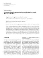
geometric interpretation refer to Figure 1.Clearly,if f
∈ C
then P
C
( f ) = f .
A well-known example of a closed convex set is a closed
linear subspace M [37, 38]ofarealHilbertspaceH. The met-
ric projection mapping P
M
is called now orthogonal projection
since the following property holds:
f − P

M
( f ),

f =0, for
all

f ∈ M,forall f ∈ H [37, 38]. Given an f

∈ H, the shift
of a closed linear subspace M by f

, that is, V := f

+ M :=
{
f

+ f : f ∈ M}, is called an (affine) linear variety [38].
Given a
/
= 0inH and ξ ∈ R,letaclosed half-space be
the closed convex set Π
+
:={

f ∈ H : a,

f ≥ξ}, that is,
Π
+

is the set of all points that lie on the “positive” side of
0
M
P
M,M

( f )
P
M
( f )
f
0
P
B[ f
0
,δ]
( f )
B[ f
0
, δ]
P
C
( f )
M

H
f
C
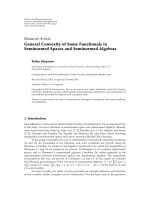
Figure 1: An illustration of the metric projection mapping P
C

onto
the closed convex subset C of H,theprojectionP
B[ f
0
,δ]
onto the
closed ball B[ f
0
, δ], the orthogonal projection P
M
onto the closed
linear subspace M, and the oblique projection P
M,M

on M along
the closed linear subspace M

.
the hyperplane Π :={

f ∈ H : a,

f =ξ},whichdefines
the boundary of Π
+
[37]. The vector a is usually called the
normal vector of Π
+
. The metric projection operator P
Π

+
can
easily be obtained by simple geometric arguments, and it is
shown to have the closed-form expression [37, 39]:
P
Π
+
( f ) = f +

ξ −a, f 

+
a
2
a, ∀f ∈ H,(3)
where τ
+
:= max{0,τ} denotes the positive part of a τ ∈ R.
Given the center

f
0
∈ H and the radius δ>0, we define
the closed ball B[

f
0
, δ]:={

f ∈ H : 


f
0
−

f ≤δ} [37].
The closed ball B[

f
0
, δ] is clearly a closed convex set, and its
metric projection mapping is given by the simple formula:
for all f
∈ H,
P
B[

f
0
,δ]
( f ) =
⎧
⎪
⎪
⎨
⎪
⎪
⎩
f ,if



f −

f
0


≤
δ,

f
0
+
δ


f −

f
0



f −

f
0

,if



f −

f
0


>δ,
(4)
which is the point of intersection of the sphere and the
segment joining f and the center of the sphere in the case
where f
/
∈B[

f
0
, δ] (see Figure 1).
Let, now, M and M

be linear subspaces of a finite-
dimensional linear subspace V
⊂ H. Then, let M + M

be
defined as the subspace M +M

:={h+h

: h ∈ M, h


∈ M

}.
If also M
∩ M

={0}, then M + M

is called the direct
sum of M and M

and is denoted by M ⊕ M

[40, 41]. In
the case where V
= M ⊕ M

, then every f ∈ V can be
expressed uniquely as a sum f
= h + h

,whereh ∈ M
and h

∈ M

[40, 41]. Then, we define here a mapping
P
M,M


: V = M ⊕ M

→ M which takes any f ∈ V to that
unique h
∈ M that appears in the decomposition f = h + h

.
We will call h the (oblique) projection of f on M along M

[40]
(see Figure 1).
4 EURASIP Journal on Advances in Signal Processing
3. CONVEX ANALYTIC VIEWPOINT OF
KERNEL-BASED CLASSIFICATION
In pattern analysis [1, 2], data are usually given by a sequence
of vectors (x
n
)
n∈Z
≥0
⊂ X ⊂ R
m
,forsomem ∈ Z
>0
.Wewill
assume that each vector in X is drawn from two classes and is
thus associated to a label y
n
∈ Y :={±1}, n ∈ Z

≥0
.Assuch,
a sequence of (training) pairs D :
= ((x
n
, y
n
))
n∈Z
≥0
⊂ X × Y
is formed.
To benefit from a larger than m or even infinite-
dimensional space, modern pattern analysis reformulates the
classification problem in an RKHS H (implicitly defined by
a predefined kernel function κ), which is widely known as
the feature space [1–3]. A mapping φ :
R
m
→ H which
takes (x
n
)
n∈Z
≥0
⊂ R
m
onto (φ(x
n
))

n∈Z
≥0
⊂ H is given by
the kernel function associated to the RKHS feature space H:
φ(x):
= κ(x, ·) ∈ H,forallx ∈ R
m
. Then, the classification
problem is defined in the feature space H as selecting a point

f ∈ H and an offset

b ∈ R such that y(

f (x)+

b) ≥ ρ,forall
(x, y)
∈ D,andforsomemargin ρ ≥ 0[1, 2].
For convenience, we merge f
∈ H and b ∈ R into a
single vector u :
= ( f , b) ∈ H × R,whereH × R stands
for the product space [37, 38]ofH and
R. Henceforth, we
will call a point u
∈ H × R a classifier,andH × R the
space of all classifiers. The space H
× R of all classifiers
can be endowed with an inner product as follows: for any

u
1
:= ( f
1
, b
1
), u
2
:= ( f
2
, b
2
) ∈ H × R,letu
1
, u
2

H×R
:=

f
1
, f
2

H
+ b
1
b
2

. The space H × R of all classifiers becomes
then a Hilbert space. The notation
·, ·will be used for both
·, ·
H×R
and ·, ·
H
.
A standard penalty function to be minimized in classifi-
cation problems is the soft margin loss function [1, 29]defined
on the space of all classifiers H
× R as follows: given a pair
(x, y)
∈ D and the margin parameter ρ ≥ 0,
l
x,y,ρ
(u):H ×R −→ R :(f , b)
  
u
−→

ρ − y

f (x)+b

+
=

ρ − yg
f ,b

(x)

+
,
(5)
where the function g
f ,b
is defined by
g
f ,b
(x):= f (x)+b, ∀x ∈ R
m
, ∀( f , b) ∈ H ×R. (6)
If the classifier
u := (

f ,

b) is such that yg

f
,

b
(x) <ρ, then this
classifier fails to achieve the margin ρ at (x, y)and(5)scoresa
penalty. In such a case, we say that the classifier committed a
margin error.Amisclassification occurs at (x, y)ifyg

f

,

b
(x) <
0.
The studies in [11, 30] approached the classification
task from a convex analytic perspective. By the definition of
the classification problem, our goal is to look for classifiers
(points in H
× R) that belong to the set Π
+
x,y,ρ
:={(

f ,

b) ∈
H × R : y(

f (x)+

b) ≥ ρ}.Ifwerecallthereproducing
property (2), a desirable classifier satisfies y(


f , κ(x, ·) +

b) ≥ ρ or 

f , yκ(x, ·)

H
+ y

b ≥ ρ. Thus, for a given
pair (x, y)andamarginρ, by the definition of the inner
product
·, ·
H×R
, the set of all desirable classifiers (that do
not commit a margin error at (x, y)) is
Π
+
x,y,ρ
=


u ∈ H ×R :


u, a
x,y

H×R
≥ ρ

,(7)
where a
x,y
:= (yκ(x, ·), y) = y(κ(x, ·),1) ∈ H × R.The
vector (κ(x,

·), 1) ∈ H ×R is an extended (to account for the
constant factor

b) vector that is completely specified by the
point x and the adopted kernel function. By (7), we notice
that Π
+
x,y,ρ
is a closed half-space of H × R (see Section 2.2).
That is, all classifiers that do not commit a margin error at
(x, y) belong in the clos ed half-space Π
+
x,y,ρ
specified by the
chosen kernel function.
The following proposition builds the bridge between the
standard loss function l
x,y,ρ
and the closed convex set Π
+
x,y,ρ
.
Proposition 1 (see [11, 30]). Given the parameters (x, y, ρ),
the closed half-space Π
+
x,y,ρ
coincides with the set of all minimiz-
ers of the soft margin loss function, that is, arg min
{l
x,y,ρ

(u):
u
∈ H ×R}=Π
+
x,y,ρ
.
Starting from this viewpoint, the following section
describes shortly a convex analytic tool [11, 30] which tackles
the online classification task, where a sequence of parameters
(x
n
, y
n
, ρ
n
)
n∈Z
≥0
, and thus a sequence of closed half-spaces
(Π
+
x
n
,y
n
,ρ
n
)
n∈Z
≥0

, is assumed.
4. THE O NLINE KERNEL-BASED CLASSIFICATION
TASK AND THE ADAPTIVE PROJECTED
SUBGRADIENT METHOD
At every time instant n
∈ Z
≥0
,apair(x
n
, y
n
) ∈ D becomes
available. If we also assume a nonnegative margin parameter
ρ
n
, then we can define the set of all classifiers that achieve this
margin by the closed half-space Π
+
x
n
,y
n
,ρ
n
:={u = (

f ,

b) ∈
H ×R : y

n
(

f (x
n
)+

b) ≥ ρ
n
}. Clearly, in an online setting, we
deal with a sequence of closed half-spaces (Π
+
x
n
,y
n
,ρ
n
)
n∈Z
≥0
⊂
H × R and since each one of them contains the set of all
desirable classifiers, our objective is to find a classifier that
belongs to or satisfies most of these half-spaces or, more
precisely, to find a classifier that belongs to all but a finite
number of Π
+
x
n

,y
n
,ρ
n
s, that is, a u ∈∩
n≥N
0
Π
+
x
n
,y
n
,ρ
n
⊂ H × R,
for some N
0
∈ Z
≥0
. In other words, we look for a classifier in
the intersection of these half-spaces.
The studies in [11, 30] propose a solution to the
above problem by the recently developed adaptive projected
subgradient method (APSM) [12–14]. The APSM approaches
the above problem as an asymptotic minimization of a
sequence of not necessarily differentiable nonnegative convex
functions over a closed convex set in a real Hilbert space.
Instead of processing a single pair (x
n

, y
n
)ateachn,
APSM offers the freedom to process concurrently a set
{(x
j
, y
j
)}
j∈J
n
, where the index set J
n
⊂ 0, n for every n ∈ Z,
and where
j
1
, j
2
:={j
1
, j
1
+1, , j
2
} for every integers
j
1
≤ j
2

. Intuitively, concurrent processing is expected to
increase the speed of an algorithm. Indeed, in adaptive
filtering [15], it is the motivation behind the leap from NLMS
[16, 17], where no concurrent processing is available, to the
potentially faster APA [18, 19].
K. Slavakis and S. Theodoridis 5
To keep the discussion simple, we assume that n ∈ J
n
,
for all n
∈ Z
≥0
. An example of such an index set J
n
is given
in (13). In other words, (13) treats the case where at time
instant n, the pairs
{(x
j
, y
j
)}
j∈n−q+1,n
,forsomeq ∈ Z
>0
,
are considered. This is in line with the basic rationale of
the celebrated affine projection algorithm (APA), which has
extremely been used in adaptive filtering [15].
Each pair (x

j
, y
j
),andthuseachindexj,definesa
half-space Π
+
x
j
,y
j
,ρ
(n)
j
by (7). In order to point out explicitly
the dependence of such a half-space on the index set J
n
,
we slightly modify the notation for Π
x
j
,y
j
,ρ
(n)
j
and use Π
+
j,n
for any j ∈ J
n

,andforanyn ∈ Z
≥0
.Themetric
projection mapping P
Π
+
j,n
is analytically given by (3). To
assign different importance to each one of the projections
corresponding to J
n
, we associate to each half-space, that
is, to each j
∈ J
n
,aweightω
(n)
j
such that ω
(n)
j
≥ 0, for
all j
∈ J
n
,and

j∈J
n
ω

(n)
j
= 1, for all n ∈ Z
≥0
. This
is in line with the adaptive filtering literature that tends
to assign higher importance in the most recent samples.
For the less familiar reader, we point out that if J
n
:=
{
n},foralln ∈ Z
≥0
, the algorithm breaks down to the
NLMS. Regarding the APA, a discussion can be found
below.
As it is also pointed out in [29, 30], the major drawback
of online kernel methods is the linear increase of complexity
with time. To deal with this problem, it was proposed in [30]
to further constrain the norm of the desirable classifiers by a
closed ball. To be more precise, one constrains the desirable
classifiers in [30]byK :
= B[0, δ] × R ⊂ H × R,forsome
predefined δ>0. As a result, one seeks for classifiers that
belong to K
∩ (

j∈J
n
, n≥N

0
Π
+
j,n
), for ∃N
0
∈ Z
≥0
. By the
definition of the closed ball B[0, δ]inSection 2.2,weeasily
see that the addition of K imposes a constraint on the norm
of

f in the vector u = (

f ,

b)by

f ≤δ. The associated
metric projection mapping is analytically given by the simple
computation P
K
(u) = (P
B[0,δ]
( f ), b), for all u := ( f , b) ∈
H ×R,whereP
B[0,δ]
is obtained by (4). It was observed that
constraining the norm results into a sequence of classifiers

with a fading memory, where old data can be eliminated
[30].
For the sake of completeness, we give a summary of the
sparsified algorithm proposed in [30].
Algorithm 1 (see [30]). For any n
∈ Z
≥0
, consider the index
set J
n
⊂ 0, n, such that n ∈ J
n
. An example of J
n
can be
foundin(13). For any j
∈ J
n
and for any n ∈ Z
≥0
, let the
closed half-space Π
+
j,n
:={u = (

f ,

b) ∈ H ×R : y
j

(

f (x
j
)+

b) ≥ ρ
(n)
j
}, and the weight ω
(n)
j
≥ 0 such that

j∈J
n
ω
(n)
j
= 1,
for all n
∈ Z
≥0
. For an arbitrary initial offset b
0
∈ R, consider
as an initial classifier the point u
0
:= (0, b
0

) ∈ H × R and
generate the following point (classifier) sequence in H
× R
by
u
n+1
:=P
K
⎛
⎝
u
n
+μ
n
⎛
⎝

j∈J
n
ω
(n)
j
P
Π
+
j,n

u
n


−
u
n
⎞
⎠
⎞
⎠
, ∀n∈Z
≥0
,
(8a)
where the extrapolation coefficient μ
n
∈ [0, 2M
n
]with
M
n
:=
⎧
⎪
⎪
⎪
⎨
⎪
⎪
⎪
⎩

j∈J

n
ω
(n)
j


P
Π
+
j,n

u
n

−u
n


2



j∈J
n
ω
(n)
j
P
Π
+

j,n

u
n

−
u
n


2
,ifu
n
/
∈

j∈J
n
Π
+
j,n
,
1, otherwise.
(8b)
Due to the convexity of
·
2
, the parameter M
n
≥ 1,

for all n
∈ Z
≥0
, so that μ
n
can take values larger than
or equal to 2. The parameters that can be preset by the
designer are the concurrency index set J
n
and μ
n
.Thebigger
the cardinality of J
n
, the more closed half-spaces to be
concurrently processed at the time instant n, which results
into a potentially increased convergence speed. An example
of J
n
, which will be followed in the numerical examples,
can be found in (13). In the same fashion, for extrapolation
parameter values μ
n
close to 2M
n
(μ
n
≤ 2M
n
), increased

convergence speed can be also observed (see Figure 6).
If we define
β
(n)
j
:= ω
(n)
j
y
j

ρ
(n)
j
− y
j
g
n

x
j

+
1+κ

x
j
, x
j


, ∀j ∈ J
n
, ∀n ∈ Z
≥0
,
(8c)
where g
n
:= g
f
n
,b
n
by (6), then the algorithmic process (8a)
can be written equivalently as follows:

f
n+1
, b
n+1

=
⎛
⎝
P
B[0,δ]
⎛
⎝
f
n

+ μ
n

j∈J
n
β
(n)
j
κ

x
j
, ·

⎞
⎠
, b
n
+ μ
n

j∈J
n
β
(n)
j
⎞
⎠
,
∀n ∈ Z

≥0
.
(8d)
The parameter M
n
takes the following form after the proper
algebraic manipulations:
M
n
:=
⎧
⎪
⎪
⎪
⎪
⎪
⎪
⎪
⎨
⎪
⎪
⎪
⎪
⎪
⎪
⎪
⎩

j∈J
n

ω
(n)
j

ρ
(n)
j
−y
j
g
n

x
j

+

2
/

1+κ

x
j
, x
j


i,j∈J
n

β
(n)
i
β
(n)
j

1+κ

x
i
, x
j

,
if u
n
/
∈

j∈J
n
Π
+
j,n
,
1, otherwise.
(8e)
As explained in [30], the introduction of the closed
ball constraint B[0, δ] on the norm of the estimates ( f

n
)
n
results into a potential elimination of the coefficients γ
n
that correspond to time instants close to index 0 in (1),
so that a buffer with length N
b
can be introduced to keep
only the most recent N
b
data (x
l
)
n
l
=n−N
b
+1
. This introduces
sparsification to the design. Since the complexity of all
the metric projections in Algorithm 1 is linear, the overall
complexity is linear on the number of the kernel function, or
after inserting the buffer with length N
b
,itisoforderO(N
b
).
4.1. Computation of the margin levels
We will now discuss in short the dynamic adjustment

strategy of the margin parameters, introduced in [11, 30].
6 EURASIP Journal on Advances in Signal Processing
For simplicity, all the concurrently processed margins are
assumed to be equal to each other, that is, ρ
n
:= ρ
(n)
j
,forall
j
∈ J
n
,foralln ∈ Z
≥0
. Of course, more elaborate schemes
can be adopted.
Whenever (ρ
n
− y
j
g
n
(x
j
))
+
= 0, the soft margin loss
function l
x
j

,y
j
,ρ
n
in (5) attains a global minimum, which
means by Proposition 1 that u
n
:= ( f
n
, b
n
)belongsto
Π
+
j,n
. In this case, we say that we have feasibility for j ∈
J
n
. Otherwise, that is, if u
n
/
∈Π
+
j,n
, infeasibility occurs. To
describe such situations, let us denote the feasibility cases by
the index set J

n
:={j ∈ J

n
:(ρ
n
− y
j
g
n
(x
j
))
+
= 0}.The
infeasibility cases are obviously J
n
\J

n
.
If we set card(∅):
= 0, then we define the feasibility rate as
the quantity R
(n)
feas
:= card(J

n
)/card(J
n
), for all n ∈ Z
≥0

.For
example, R
(n)
feas
= 1/2 denotes that the number of feasibility
cases is equal to the number of infeasibility ones at the time
instant n
∈ Z
≥0
.
If, at time n, R
(n)
feas
is larger than or equal to some
predefined R, we assume that this will also happen for the
next time instant n+1, provided we work in a slowly changing
environment. More than that, we expect R
(n+1)
feas
≥ R to hold
for a margin ρ
n+1
slightly larger than ρ
n
.Hence,attimen,if
R
(n)
feas
≥ R,wesetρ
n+1

>ρ
n
under some rule to be discussed
below. On the contrary, if R
(n)
feas
<R, then we assume that if
the margin parameter value is slightly decreased to ρ
n+1
<ρ
n
,
it may be possible to have R
(n+1)
feas
≥ R. For example, if we
set R :
= 1/2, this scheme aims at keeping the number of
feasibility cases larger than or equal to those of infeasibilities,
while at the same time it tries to push the margin parameter
to larger values for better classification at the test phase.
In the design of [11, 30], the small variations of the
parameters (ρ
n
)
n∈Z
≥0
are controlled by the linear parametric
model ν
APSM

(θ − θ
0
)+ρ
0
, θ ∈ R,whereθ
0
, ρ
0
∈ R, ρ
0
≥ 0,
are predefined parameters and ν
APSM
is a sufficiently small
positive slope (e.g., see Section 7). For example, in [30],
ρ
n
:= (ν
APSM
(θ
n
− θ
0
)+ρ
0
)
+
,whereθ
n+1
:= θ

n
± δθ,forall
n, and where the
± symbol refers to the dichotomy of either
R
(n+1)
feas
≥ R or R
(n+1)
feas
<R. In this way, an increase of θ by
δθ > 0 will increase ρ, whereas a decrease of θ by
−δθ will
force ρ to take smaller values. Of course, other models, other
than this simple linear one, can also be adopted.
4.2. Kernel affine projection algorithm
Here we introduce a byproduct of Algorithm 1,namely,a
kernelized version of the standard affine projection algo-
rithm [15, 18, 19].
Motivated by the discussion in Section 3, Algorithm 1
was devised in order to find at each time instant n a point
in the set of all desirable classifiers

j∈Jn
Π
+
j,n
/
= ∅. Since any
point in this intersection is suitable for the classification task

at time n, any nonempty subset of

j∈J
n
Π
+
j,n
can be used for
the problem at hand. In what follows we see that if we limit
the set of desirable classifiers and deal with the boundaries
{Π
j,n
}
j∈J
n
, that is, hyperplanes (Section 2.2), of the closed
half-spaces
{Π
+
j,n
}
j∈J
n
, we end up with a kernelized version
of the classical affine projection algorithm [18, 19].
Π
1,n
Π
+
1,n

Π
+
1,n
∩Π
+
2,n
u
n
+ μ
n
(

2
j
=1
ω
(n)
j
P
Π
+
j,n
(u
n
) −u
n
)
P
Π
+

1,n
(u
n
)
V
n
P
V
n
(u
n
)
P
Π
+
2,n
(u
n
)
u
n
Π
2,n
Π
+
2,n
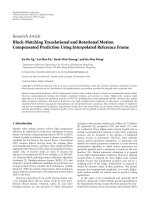
Figure 2: For simplicity, we assume that at some time instant n ∈
Z
≥0
, the cardinality card(J

n
) = 2. This figure illustrates the closed
half-spaces
{Π
+
j,n
}
2
j
=1
and their boundaries, that is, the hyperplanes
{Π
j,n
}
2
j
=1
. In the case where

2
j
=1
Π
j,n
/
= ∅, the defined in (11)
linear variety becomes V
n
=


2
j
=1
Π
j,n
, which is a subset of

2
j
=1
Π
+
j,n
.
The kernel APA aims at finding a point in the linear variety V
n
,
while Algorithm 1 and the APSM consider the more general setting
of finding a point in

2
j
=1
Π
+
j,n
.Duetotherangeoftheextrapolation
parameter μ
n
∈ [0, 2M

n
]andM
n
≥ 1, the APSM can rapidly
furnish solutions close to the large intersection of the closed half-
spaces (see also Figure 6), without suffering from instabilities in the
calculation of a Moore-Penrose pseudoinverse matrix necessary for
finding the projection P
V
n
.
Definition 1 (kernel affine projection algorithm). Fix n ∈
Z
≥0
and let q
n
:= card(J
n
). Define the set of hyperplanes
{Π
j,n
}
j∈J
n
by
Π
j,n
:=

(


f ,

b)∈H ×R :

(

f ,

b),

y
j
κ

x
j
, ·

, y
j

H×R
=ρ
(n)
j

=



u ∈ H ×R :


u, a
j,n

H×R
= ρ
(n)
j

, ∀j ∈ J
n
,
(9)
where a
j,n
:= y
j
(κ(x
j
, ·), 1), for all j ∈ J
n
. These hyper-
planes are the boundaries of the closed half-spaces
{Π
+
j,n
}
j∈J

n
(see Figure 2).Notethatsuchhyperplaneconstraintsasin
(9) are often met in regression problems with the difference
that there the coefficients
{ρ
(n)
j
}
j∈J
n
are part of the given data
and not parameters as in the present classification task.
Since we will be looking for classifiers in the assumed
nonempty intersection

j∈J
n
Π
j,n
, we define the function
e
n
: H ×R → R
q
n
by
e
n
(u):=
⎡

⎢
⎢
⎢
⎣
ρ
(n)
1
−

a
1,n
, u

.
.
.
ρ
(n)
q
n
−

a
q
n
,n
, u

⎤
⎥

⎥
⎥
⎦
, ∀u ∈ H ×R, (10)
and let the set (see Figure 2)
V
n
:= arg min
u∈H×R
q
n

j=1


ρ
(n)
j
−

u, a
j,n



2
= arg min
u∈H×R



e
n
(u)


2
R
q
n
.
(11)
This set is a linear variety (for a proof see Appendix A).
Clearly, if

j∈J
n
Π
j,n
/
= ∅, then V
n
=

j∈J
n
Π
j,n
.Now,given
K. Slavakis and S. Theodoridis 7
an arbitrary initial u

0
, the kernel affine projection algorithm is
defined by the following point sequence:
u
n+1
:= u
n
+ μ
n

P
V
n

u
n

−
u
n

=
u
n
+ μ
n

a
1,n
, , a

q
n
,n

G
†
n
e
n

u
n

, ∀n ∈ Z
≥0
,
(12)
where the extrapolation parameter μ
n
∈ [0, 2], G
n
is a matrix
of dimension q
n
×q
n
,whereits(i, j)th element is defined by
y
i
y

j
(κ(x
i
, x
j
)+1),foralli, j ∈ 1, q
n
, the symbol † stands for
the (Moore-Penrose) pseudoinverse operator [40], and the
notation (a
1,n
, , a
q
n
,n
)λ :=

q
n
j=1
λ
j
a
j,n
,forallλ ∈ R
q
n
.For
the proof of the equality in (12), refer to Appendix A.
Remark 1. The fact that the classical (linear kernel) APA

[18, 19] can be seen as a projection algorithm onto a
sequence of linear varieties was also demonstrated in
[26, Appendix B]. The proof in Appendix A extends the
defining formula of the APA, and thus the proof given in [26,
Appendix B], to infinite-dimensional Hilbert spaces. Extend-
ing [26], the APSM [12–14] devised a convexly constrained
asymptotic minimization framework which contains APA,
the NLMS, as well as a variety of recently developed
projection-based algorithms [20–25, 27, 28].
By Definition 1 and Appendix A, at each time instant
n, the kernel APA produces its estimate by projecting onto
the linear variety V
n
. In the special case where q
n
:= 1,
that is, J
n
={n},foralln, then (12) gives the kernel
NLMS [42]. Note also that in this case, the pseudoinverse
is simplified to G
†
n
= a
n
/a
n

2
,foralln. Since V

n
is a
closed convex set, the kernel APA can be included in the
wide frame of the APSM (see also the remarks just after
Lemma 3.3 or Example 4.3 in [14]). Under the APSM frame,
more directions become available for the kernel APA, not
only in terms of theoretical properties, but also in devising
variations and extensions of the kernel APA by considering
more general convex constraints than V
n
as in [26], and by
incorporating a priori information about the model under
study [14].
Note that in the case where

j∈J
n
Π
j,n
/
= ∅, then V
n
=

j∈J
n
Π
j,n
. Since Π
j,n

is the boundary and thus a subset
of the closed half-space Π
+
j,n
, it is clear that looking for
points in

j∈J
n
Π
j,n
, in the kernel APA and not in the larger

j∈J
n
Π
+
j,n
as in Algorithm 1, limits our view of the online
classification task (see Figure 2). Under mild conditions,
Algorithm 1 produces a point sequence that enjoys prop-
erties like monotone approximation, strong convergence to
a point in the intersection K
∩ (

j∈J
n
Π
+
j,n

), asymptotic
optimality, as well as a characterization of the limit point.
To speed up convergence, Algorithm 1 offers the extrapo-
lation parameter μ
n
which has a range of μ
n
∈ [0, 2M
n
]with
M
n
≥ 1. The calculation of the upper bound M
n
is given by
simple operations that do not suffer by instabilities as in the
computation of the (Moore-Penrose) pseudoinverses (G
†
n
)
n
in (12)[40]. A usual practice for the efficient computation of
the pseudoinverse matrix is to diagonally load some matrix
with positive values prior inversion, leading thus to solutions
towards an approximation of the original problem at hand
[15, 40].
The above-introduced kernel APA is based on the
fundamental notion of metric projection mapping on linear
varieties in a Hilbert space, and it can thus be straightfor-
wardly extended to regression problems. In the sequel, we

willfocusonthemoregeneralviewoffered to classification
by Algorithm 1 and not pursue further the kernel APA
approach.
5. SPARSIFICATION BY A SEQUENCE OF
FINITE-DIMENSIONAL SUBSPACES
In this section, sparsification is achieved by the construction
of a sequence of linear subspaces (M
n
)
n∈Z
≥0
, together with
their bases (B
n
)
n∈Z
≥0
, in the space H. The present approach
is in line with the rationale presented in [36], where a
monotonically increasing sequence of subspaces (M
n
)
n∈Z
≥0
was constructed, that is, M
n
⊆ M
n+1
,foralln ∈ Z
≥0

.
Such a monotonic increase of the subspaces’ dimension
undoubtedly raises memory resources issues. In this paper,
such a monotonicity restriction is not followed.
To accomodate memory limitations and tracking
requirements, two parameters, namely L
b
and α,willbe
of central importance in our design. The parameter L
b
establishes a bound on the dimensions of (M
n
)
n∈Z
≥0
, that is,
if we define L
n
:= dim(M
n
), then L
n
≤ L
b
,foralln ∈ Z
≥0
.
Given a basis B
n
,abuffer is needed in order to keep track

of the L
n
basis elements. The larger the dimension for the
subspace M
n
, the larger the buffer necessary for saving the
basis elements. Here, L
b
gives the designer the freedom
to preset an upper bound for the dimensions (L
n
)
n
,and
thus upper-bound the size of the buffer according to the
available computational resources. Note that this introduces
atradeoff between memory savings and representation
accuracy; the larger the buffer, the more basis elements
to be used in the kernel expansion, and thus the larger
the accuracy of the functional representation, or, in other
words, the larger the span of the basis, which gives us more
candidates for our classifier. We will see below that such
aboundL
b
results into a sliding window effect. Note also
that if the data
{x
n
}
n∈Z

≥0
are drawn from a compact set
in
R
m
, then the algorithmic procedure introduced in [36]
produces a sequence of monotonically increasing subspaces
with dimensions upper-bounded by some bound not known
apriori.
The parameter α is a measure of approximate lin-
ear dependency or independency. Every time a new ele-
ment κ(x
n+1
, ·) becomes available, we compare its dis-
tance from the available finite-dimensional linear sub-
space M
n
= span(B
n
)withα, where span stands
for the linear span operation. If the distance is larger
than α, then we say that κ(x
n+1
, ·)issufficiently linearly
independent of the basis elements of B
n
, we decide that it
carries enough “new information,” and we add this element
to the basis, creating a new B
n+1

which clearly contains
B
n
. However, if the above distance is smaller than or equal
to α, then we say that κ(x
n+1
, ·) is approximately linearly
dependent on the elements of B
n
, so that augmenting B
n
8 EURASIP Journal on Advances in Signal Processing
is not needed. In other words, α controls the frequency by
which new elements enter the basis. Obviously, the larger the
α, the more “difficult” for a new element to contribute to the
basis. Again, a tradeoff between the cardinality of the basis
and the functional representation accuracy is introduced, as
also seen above for the parameter L
b
.
To increase the speed of convergence of the proposed
algorithm, concurrent processing is introduced by means of
the index set J
n
, which indicates which closed half-spaces
will be processed at the time instant n. Note once again that
such a processing is behind the increase of the convergence
speed met in APA [18, 19] when compared to that of the
NLMS [16, 17], in classical adaptive filtering [15]. Without
any loss of generality, and in order to keep the discussion

simple, we consider here the following simple case for J
n
:
J
n
:=

0, n,ifn<q−1,
n − q +1,n,ifn ≥ q − 1,
∀n ∈ Z
≥0
, (13)
where q
∈ Z
>0
is a predefined constant denoting the number
of closed half-spaces to be processed at each time instant n
≥
q − 1. In other words, for n ≥ q − 1, at each time instant n,
we consider concurrent projections on the closed half-spaces
associated with the q most recent samples. We state now a
definition whose motivation is the geometrical framework of
the oblique projection mapping given in Figure 1.
Definition 2. Given n
∈ Z
≥0
, assume the finite-dimensional
linear subspaces M
n
, M

n+1
⊂ H with dimensions L
n
and
L
n+1
, respectively. Then it is well known that there exists a
linear subspace W
n
, such that M
n
+M
n+1
= W
n
⊕M
n+1
,where
the symbol
⊕ stands for the direct sum [40, 41]. Then, the
following mapping is defined:
π
n
: M
n
+ M
n+1
−→ M
n+1
: f −→ π

n
( f ):=

f ,ifM
n
⊆ M
n+1
P
M
n+1
,W
n
( f ), if M
n
/
⊆M
n+1
,
(14)
where P
M
n+1
,W
n
denotes the oblique projection mapping on
M
n+1
along W
n
. To visualize this in the case when M

n
/
⊆M
n+1
,
refer to Figure 1,whereM becomes M
n+1
,andM

becomes
W
n
.
To exhibit the sparsification method, the constructive
approach of mathematical induction on n
∈ Z
≥0
is used as
follows.
5.1. Initialization
Let us begin, now, with the construction of the bases
(B
n
)
n∈Z
≥0
and the linear subspaces (M
n
)
n∈Z

≥0
. At the starting
time 0, our basis B
0
consists of only one vector ψ
(0)
1
:=
κ(x
0
, ·) ∈ H, that is, B
0
:={ψ
(0)
1
}. This basis defines the
linear subspace M
0
:= span(B
0
). The characterization of the
element κ(x
0
, ·) by the basis B
0
is obvious here: κ(x
0
, ·) =
1·ψ
(0)

1
. Hence, we can associate to κ(x
0
, ·) the one-dimen-
sional vector θ
(0)
x
0
:= 1, which completely describes κ(x
0
, ·)by
the basis B
0
. Let also K
0
:= κ(x
0
, x
0
) > 0, which guarantees
the existence of the inverse K
−1
0
= 1/κ(x
0
, x
0
).
5.2. At the time instant n
∈ Z

>0
We assume, now, that at time n ∈ Z
>0
the basis B
n
=
{
ψ
(n)
1
, , ψ
(n)
L
n
} is available, where L
n
∈ Z
>0
. Define also the
linear subspace M
n
:= span(B
n
), which is of dimension L
n
.
Without loss of generality, we assume that n
≥ q − 1, so
that the index set J
n

:= n − q +1,n is available. Available are
also the kernel functions
{κ(x
j
, ·)}
j∈J
n
. Our sparsification
method is built on the sequence of closed linear subspaces
(M
n
)
n
. At every time instant n, all the information needed for
the realization of the sparsification method will be contained
within M
n
.Assuch,eachκ(x
j
, ·), for j ∈ J
n
,mustbe
associated or approximated by a vector in M
n
.Thus,we
associate to each κ(x
j
, ·), j ∈ J
n
, a set of vectors {θ

(n)
x
j
}
j∈J
n
,
as follows
κ

x
j
, ·

−→ k
(n)
x
j
:=
L
n

l=1
θ
(n)
x
j
,l
ψ
(n)

l
∈ M
n
, ∀j ∈ J
n
. (15)
For example, at time 0, κ(x
0
, ·) → k
(0)
x
0
:= ψ
(0)
1
. Since we
follow the constructive approach of mathematical induction,
the above set of vectors is assumed to be known.
Available is also the matrix K
n
∈ R
L
n
×L
n
whose (i, j)th
component is (K
n
)
i,j

:=ψ
(n)
i
, ψ
(n)
j
,foralli, j ∈ 1, L
n
.Itcan
be readily verified that K
n
is a Gram matrix which, by the
assumption that
{ψ
(n)
l
}
L
n
l=1
are linearly independent, is also
positive definite [40, 41]. Hence, the existence of its inverse
K
−1
n
is guaranteed. We assume here that K
−1
n
is also available.
5.3. At time n +1, the new data x

n+1
becomes available
At time n + 1, a new element κ(x
n+1
, ·)ofH becomes
available. Since M
n
is a closed linear subspace of H, the
orthogonal projection of κ(x
n+1
, ·)ontoM
n
is well defined
and given by
P
M
n

κ

x
n+1
, ·

=
L
n

l=1
ζ

(n+1)
x
n+1
,l
ψ
(n)
l
∈ M
n
, (16)
where the vector ζ
(n+1)
x
n+1
:= [ζ
(n+1)
x
n+1
,1
, , ζ
(n+1)
x
n+1
,L
n
]
t
∈ R
L
n

satisfies
the normal equations K
n
ζ
(n+1)
x
n+1
= c
(n+1)
x
n+1
with c
(n+1)
x
n+1
given by
[37, 38]
c
(n+1)
x
n+1
:=
⎡
⎢
⎢
⎢
⎣

κ


x
n+1
, ·

, ψ
(n)
1

.
.
.

κ

x
n+1
, ·

, ψ
(n)
L
n

⎤
⎥
⎥
⎥
⎦
∈ R
L

n
. (17)
Since K
−1
n
was assumed available, we can compute ζ
(n+1)
x
n+1
by
ζ
(n+1)
x
n+1
= K
−1
n
c
(n+1)
x
n+1
. (18)
Now, the distance d
n+1
of κ(x
n+1
, ·)fromM
n
(in Figure 1
this is the quantity

f −P
M
( f )) can be calculated as follows:
0
≤ d
2
n+1
:=


κ

x
n+1
, ·

−P
M
n

κ

x
n+1
, ·



2
= κ


x
n+1
, x
n+1

−

c
(n+1)
x
n+1

t
ζ
(n+1)
x
n+1
.
(19)
In order to derive (19), we used the fact that the linear oper-
ator P
M
n
is selfadjoint and the linearity of the inner product
·, · [37, 38]. Let us define now B
n+1
:={ψ
(n+1)
l

}
L
n+1
l=1
.
K. Slavakis and S. Theodoridis 9
5.3.1. Approximate linear dependency (d
n+1
≤ α)
If the metric distance of κ(x
n+1
, ·)fromM
n
satisfies d
n+1
≤ α,
then we say that κ(x
n+1
, ·)isapproximately linearly dependent
on B
n
:={ψ
(n)
l
}
L
n
l=1
, and that it is not necessary to insert
κ(x

n+1
, ·) into the new basis B
n+1
. That is, we keep B
n+1
:=
B
n
, which clearly implies that L
n+1
:= L
n
,andψ
(n+1)
l
:= ψ
(n)
l
,
for all l
∈ 1, L
n
.Moreover,M
n+1
:= span(B
n+1
) = M
n
. Also,
we let K

n+1
:= K
n
,andK
−1
n+1
:= K
−1
n
.
Notice here that J
n+1
:= n − q +2,n + 1. The approxi-
mations given by (15) have to be transfered now to the new
linear subspace M
n+1
. To do so, we employ the mapping π
n
given in Definition 2:forallj ∈ J
n+1
\{n +1}, k
(n+1)
x
j
:=
π
n
(k
(n)
x

j
). Since, M
n+1
= M
n
, then by (14),
k
(n+1)
x
j
:= π
n

k
(n)
x
j

=
k
(n)
x
j
. (20)
As a result, θ
(n+1)
x
j
:= θ
(n)

x
j
,forallj ∈ J
n
\{n +1}.As
for k
(n+1)
x
n+1
, we use (16) and let k
(n+1)
x
n+1
:= P
M
n
(κ(x
n+1
, ·)). In
other words, κ(x
n+1
, ·) is approximated by its orthogonal
projection P
M
n
(κ(x
n+1
, ·)) onto M
n
, and this information is

kept in memory by the coefficient vector θ
(n+1)
x
n+1
:= ζ
(n+1)
x
n+1
.
5.3.2. Approximate linear independency (d
n+1
>α)
On the other hand, if d
n+1
>α, then κ(x
n+1
, ·)becomes
approximately linearly independent on B
n
,andweaddit
to our new basis. If we also have L
n
≤ L
b
− 1, then we
can increase the dimension of the basis without exceeding
the memory of the buffer: L
n+1
:= L
n

+1andB
n+1
:=
B
n
∪{κ(x
n+1
, ·)}, such that the elements {ψ
(n+1)
l
}
L
n+1
l=1
of B
n+1
become ψ
(n+1)
l
:= ψ
(n)
l
,foralll ∈ 1,L
n
,andψ
(n+1)
L
n+1
:=
κ(x

n+1
, ·). We also update the Gram matrix by
K
n+1
:=
⎡
⎣
K
n
c
(n+1)
x
n+1

c
(n+1)
x
n+1

t
κ

x
n+1
, x
n+1

⎤
⎦
=

:
⎡
⎣
r
n+1
h
t
n+1
h
n+1
H
n+1
⎤
⎦
.
(21)
The fact d
n+1
>α≥ 0 guarantees that the vectors in B
n+1
are linearly independent. In this way the Gram matrix K
n+1
is positive definite. It can be verified by simple algebraic
manipulations that
K
−1
n+1
=
⎡
⎢

⎢
⎢
⎢
⎢
⎣
K
−1
n
+
ζ
(n+1)
x
n+1

ζ
(n+1)
x
n+1

t
d
2
n+1
−
ζ
(n+1)
x
n+1
d
2

n+1
−

ζ
(n+1)
x
n+1

t
d
2
n+1
1
d
2
n+1
⎤
⎥
⎥
⎥
⎥
⎥
⎦
=
:

s
n+1
p
t

n+1
p
n+1
P
n+1

.
(22)
Since B
n
 B
n+1
, we immediately obtain that M
n

M
n+1
. All the information given by (15) has to be translated
now to the new linear subspace M
n+1
by the mapping π
n
as
we did above in (20): k
(n+1)
x
j
:= π
n
(k

(n)
x
j
) = k
(n)
x
j
. Since the
cardinality of B
n+1
is larger than the cardinality of B
n
by
one, then θ
(n+1)
x
j
= [(θ
(n)
x
j
)
t
,0]
t
,forallj ∈ J
n+1
\{n +1}.
The new vector κ(x
n+1

, ·), being a basis vector itself, satisfies
κ(x
n+1
, ·) ∈ M
n+1
, so that k
(n+1)
x
n+1
:= κ(x
n+1
, ·). Hence, it has
the following representation with respect to the new basis
B
n+1
: θ
(n+1)
x
n+1
:= [0
t
,1]
t
∈ R
L
n+1
.
5.3.3. Approximate linear independency (d
n+1
>α)

and buffer overflow (L
n
+1>L
b
); the sliding
window effect
Now, assume that d
n+1
>αand that L
n
= L
b
. According
to the above methodology, we still need to add κ(x
n+1
, ·)to
our new basis, but if we do so the cardinality L
n
+ 1 of this
new basis will exceed our buffer’s memory L
b
. We choose
here to discard the oldest element ψ
(n)
1
in order to make
space for κ(x
n+1
, ·): B
n+1

:= (B
n
\{ψ
(n)
1
}) ∪{κ(x
n+1
, ·)}.
This discard of ψ
(n)
1
and the addition of κ(x
n+1
, ·) results
in the sliding window effect. We stress here that instead of
discarding ψ
(n)
1
, other elements of B
n
can be removed, if we
use different criteria than the present ones. Here, we choose
ψ
(n)
1
for simplicity, and for allowing the algorithm to focus
on recent system changes by making its dependence on the
remote past diminishing as time moves on.
We de fine h ere L
n+1

:= L
b
, such that the elements of B
n+1
become ψ
(n+1)
l
:= ψ
(n)
l+1
, l ∈ 1, L
b
−1, and ψ
(n+1)
L
b
:= κ(x
n+1
, ·).
In this way, the update for the Gram matrix becomes K
n+1
:=
H
n+1
by (21), where it can be verified that
K
−1
n+1
= H
−1

n+1
= P
n+1
−
1
s
n+1
p
n+1
p
t
n+1
, (23)
where P
n+1
is defined by (22) (the proof of (23)isgivenin
Appendix B).
Upon defining M
n+1
:= span(B
n+1
), it is easy to see that
M
n
/
⊆M
n+1
. By the definition of the oblique projection, of the
mapping π
n

,andbyk
(n)
x
j
:=

L
n
l=1
θ
(n)
x
j
,l
ψ
(n)
l
,forallj ∈ J
n+1
\
{
n +1},weobtain
k
(n+1)
x
j
:= π
n

k

(n)
x
j

=
L
n

l=2
θ
(n)
x
j
,l
ψ
(n)
l
+0·κ

x
n+1
, ·

=
L
n+1

l=1
θ
(n+1)

x
j
,l
ψ
(n+1)
l
, ∀j ∈ J
n+1
\{n +1},
(24)
where θ
(n+1)
x
j
,l
:= θ
(n)
x
j
,l+1
,foralll ∈ 1, L
b
−1, and θ
(n+1)
x
j
,L
b
:= 0,
for all j

∈ J
n+1
\{n +1}. Since κ(x
n+1
, ·) ∈ M
n+1
,weset
k
(n+1)
x
n+1
:= κ(x
n+1
, ·) with the following representation with
respect to the new basis B
n+1
: θ
(n+1)
x
n+1
:= [0
t
,1]
t
∈ R
L
b
.The
sparsification scheme can be found in pseudocode format in
Algorithm 2.

6. THE APSM WITH THE SUBSPACE-BASED
SPARSIFICATION
In this section, we embed the sparsification strategy of
Section 5 in the APSM. As a result, the following algorithmic
procedure is obtained.
10 EURASIP Journal on Advances in Signal Processing
Subalgorithm
1. Initialization.LetB
0
:={κ(x
0
, ·)}, K
0
:= κ(x
0
, x
0
) > 0,
and K
−1
0
:= 1/κ(x
0
, x
0
). Also, J
0
:={0}, θ
(0)
x

0
:= 1, and
γ
(0)
1
:= 0. Fix α ≥ 0, and L
b
∈ Z
>0
.
2. Assume n
∈ Z
>0
. Available are B
n
, {θ
(n)
x
j
}
j∈J
n
,where
J
n
:= n − q +1,n,aswellasK
n
∈ R
L
n

×L
n
, K
−1
n
∈ R
L
n
×L
n
,
and the coefficients
{γ
(n+1)
l
}
L
n
l=1
for the estimate in (26).
3.Timebecomesn +1,andκ(x
n+1
, ·) arrives. Notice that
J
n+1
:= n − q +2,n +1.
4.Calculatec
(n+1)
x
n+1

and ζ
(n+1)
x
n+1
by (17) and (18), respectively,
and the distance d
n+1
by (19).
5. if d
n+1
≤ α then
6. L
n+1
:= L
n
.
7.SetB
n+1
:= B
n
.
8.Letθ
(n+1)
x
j
:= θ
(n)
x
j
,forallj ∈ J

n+1
\{n +1},and
θ
(n+1)
x
n+1
:= ζ
(n+1)
x
n+1
.
9. K
n+1
:= K
n
,andK
−1
n+1
:= K
−1
n
.
10.Let
{γ
(n+2)
l
}
L
n+1
l=1

:={

γ
(n+1)
l
}
L
n
l=1
.
11. else
12. if L
n
≤ L
b
−1 then
13. L
n+1
:= L
n
+1.
14.SetB
n+1
:= B
n
∪{κ(x
n+1
, ·)}.
15.Letθ
(n+1)

x
j
:= [(θ
(n)
x
j
)
t
,0]
t
,forallj ∈ J
n+1
\{n +1},
and θ
(n+1)
x
n+1
:= [0
t
,1]
t
∈ R
L
n
+1
.
16. Define K
n+1
and its inverse K
−1

n+1
by (21) and (22),
respectively.
17.
γ
(n+2)
l
:= γ
(n+1)
l
+ μ
n+1

j∈J
n+1

β
(n+1)
j
θ
(n+1)
x
j
,l
,forall
l
∈ 1, L
n+1
−1, and γ
(n+2)

L
n+1
:= μ
n+1

β
(n+1)
n+1
θ
(n+1)
x
n+1
,L
n+1
.
18. else if L
n
= L
b
then
19. L
n+1
:= L
b
.
20.LetB
n+1
:= (B
n
\{ψ

(n)
1
}) ∪{κ(x
n+1
, ·)}.
21.Setθ
(n+1)
x
j
,l
= θ
(n)
x
j
,l+1
,foralll ∈ 1, L
b
−1, and
θ
(n+1)
x
j
,L
b
:= 0, for all j ∈ J
n+1
\{n +1}.Moreover,
θ
(n+1)
x

n+1
:= [0
t
,1]
t
∈ R
L
b
.
22.SetK
n+1
:= H
n+1
by (21). Then, K
−1
n+1
is given by
(23).
23.
γ
(n+2)
l
:= γ
(n+1)
l+1
+ μ
n+1

j∈J
n+1


β
(n+1)
j
θ
(n+1)
x
j
,l
,forall
l
∈ 1, L
n+1
−1, and γ
(n+2)
L
n+1
:= μ
n+1

β
(n+1)
n+1
θ
(n+1)
x
n+1
,L
n+1
.

24. end
25. Increase n by one, that is, n
← n +1andgotoline2.
Algorithm 2: Sparsification scheme by a sequence of finite-dimen-
sional linear subspaces.
Algorithm 3 .Foranyn ∈ Z
≥0
, consider the index set J
n
defined by (13). For any j ∈ J
n
and for any n ∈ Z
≥0
,
let the closed half-space Π
+
j,n
:={u = (

f ,

b) ∈ H × R :
y
j
(

f (x
j
)+


b) ≥ ρ
(n)
j
} and the weight ω
(n)
j
≥ 0 such that

j∈J
n
ω
(n)
j
= 1. For an arbitrary initial offset

b
0
∈ R, consider
as an initial classifier the point
u
0
:= (0,

b
0
) ∈ H × R and
generate the following sequences by

f
n+1

:= π
n−1


f
n

+ μ
n

j∈J
n

β
(n)
j
k
(n)
x
j
(25a)
= π
n−1


f
n

+
L

n

l=1


μ
n

j∈J
n

β
(n)
j
θ
(n)
x
j
,l

ψ
(n)
l
, ∀n ∈ Z
≥0
,
(25b)
where π
−1
(


f
0
):= 0, the vectors {θ
(n)
x
j
}
j∈J
n
,foralln ∈ Z
≥0
,
are given by Algorithm 2,and

b
n+1
:=

b
n
+ μ
n

j∈J
n

β
(n)
j

, ∀n ∈ Z
≥0
, (25c)
where

β
(n)
j
:= ω
(n)
j
y
j

ρ
n
− y
j
g
n

x
j

+
1+κ

x
j
, x

j

, ∀n ∈ Z
≥0
. (25d)
The function
g
n
:= g

f
n
,

b
n
,andg is defined by (6). Moreover
ρ
n
is given by the procedure described in Section 4.1. Also,
μ
n
∈ [0, 2

M
n
], where

M
n

:=
⎧
⎪
⎪
⎪
⎪
⎪
⎪
⎪
⎨
⎪
⎪
⎪
⎪
⎪
⎪
⎪
⎩

j∈J
n
ω
(n)
j

ρ
n
−y
j
g

n

x
j

+

2
/

1+κ

x
j
, x
j


i,j∈J
n

β
(n)
i

β
(n)
j

1+κ


x
j
, x
j

,
if
u
n
:=


f
n
,

b
n

/
∈

j∈J
n
Π
+
j,n
,
1, otherwise,

∀n ∈ Z
≥0
.
(25e)
The following proposition holds.
Proposition 2. Let the sequence of estimates (

f
n
)
n∈Z
≥0
obtain-
ed by Algorithm 3.Then,foralln
∈ Z
≥0
, there exists
(γ
(n)
l
)
L
n−1
l=1
⊂ R such that

f
n
=
L

n−1

l=1
γ
(n)
l
ψ
(n−1)
l
∈ M
n−1
, ∀n ∈ Z
≥0
, (26)
where B
−1
:={0}, M
−1
:={0},andL
−1
:= 1.
Proof. See Appendix C.
Now that we have a kernel series expression for the
estimate

f
n
by (26), we can give also an expression for the
quantity π
n−1

(

f
n
)in(25b), by using also the definition (14):
π
n−1


f
n

=
⎧
⎪
⎪
⎪
⎨
⎪
⎪
⎪
⎩

f
n
,ifM
n−1
⊆ M
n
,

L
n−1

l=2
γ
(n)
l
ψ
(n−1)
l
,ifM
n−1
/
⊆M
n
.
(27)
That is, whenever M
n−1
/
⊆M
n
,weremovefromthekernel
series expansion (26) the term corresponding to the basis
element ψ
(n−1)
1
. This is due to the sliding window effect and
K. Slavakis and S. Theodoridis 11
1. Initialization.LetB

0
:={κ(x
0
, ·)}, θ
(0)
x
0
:= 1, γ
(0)
1
:= 0,
J
0
:={0},and choose for the initial offset

b
0
any value
in
R.Fixα ≥ 0andL
b
∈ Z
>0
.
2. Assume the time instant n
∈ Z
>0
.Now, the index set J
n
becomes J

n
:= n − q +1,n by (13). We already know
B
n−1
, {θ
(n−1)
x
j
}
j∈J
n−1
,as well as {γ
(n)
l
}
L
n−1
l=1
and

b
n
.
3. Calculate the new basis B
n
,and the vectors {θ
(n)
x
j
}

j∈J
n
by
Algorithm 2.
4.Compute
{

β
(n)
j
}
j∈J
n
by (25d).
5. Choose an extrapolation parameter value μ
n
from the
interval [0, 2

M
n
],where

M
n
is computed by (25e).
6.Calculatethecoefficients
{γ
(n+1)
l

}
L
n
l=1
by (28).
7. The classifier (

f
n+1
,

b
n+1
)isgivenby(26) and (25c).
8. Increase n by one, that is, n
← n +1andgotoline2.
Algorithm 3: Proposed algorithm.
refers to the case of Section 5.3.3. According to our strategy,
the case M
n−1
/
⊆M
n
happens only when approximate linear
independency d
n
>αand a buffer overflow L
n−1
+1 >L
b

occurs. To prevent this buffer overflow, we have to cut off the
term corresponding to ψ
(n−1)
1
, and keep an empty position in
the buffer in order for the new element κ(x
n
, ·)tocontribute
to the basis. Having the knowledge of (27), the coefficients
{γ
(n)
l
}
L
n−1
l=1
,foralln ∈ Z
≥0
, will be given by the following
iterative formula: let
γ
(0)
1
:= 0, and for all n ∈ Z
≥0
,

γ
(n+1)
l


L
n
l=1
:=
⎧
⎪
⎪
⎪
⎪
⎪
⎪
⎪
⎪
⎪
⎪
⎪
⎪
⎪
⎪
⎪
⎪
⎪
⎪
⎪
⎪
⎪
⎪
⎪
⎪

⎨
⎪
⎪
⎪
⎪
⎪
⎪
⎪
⎪
⎪
⎪
⎪
⎪
⎪
⎪
⎪
⎪
⎪
⎪
⎪
⎪
⎪
⎪
⎪
⎪
⎩

γ
(n)
l

+ μ
n

j∈J
n

β
(n)
j
θ
(n)
x
j
,l
, ∀l ∈ 1, L
n
,
if d
n
≤ α,
⎧
⎪
⎪
⎨
⎪
⎪
⎩

γ
(n)

l
+ μ
n

j∈J
n

β
(n)
j
θ
(n)
x
j
,l
, ∀l ∈ 1, L
n
−1,
μ
n

β
(n)
n
θ
(n)
x
n
,L
n

, l = L
n
,
if d
n
>α, L
n−1
+1≤ L
b
,
⎧
⎪
⎪
⎨
⎪
⎪
⎩

γ
(n)
l+1
+ μ
n

j∈J
n

β
(n)
j

θ
(n)
x
j
,l
, ∀l ∈ 1, L
n
−1,
μ
n

β
(n)
n
θ
(n)
x
n
,L
n
, l = L
n
,
if d
n
>α, L
n−1
+1>L
b
.

(28)
Our proposed algorithm is summarized as shown in
Algorithm 3.
Notice that the calculation of all the metric and oblique
projections is of linear complexity with respect to the
dimension L
n
. The main computational load of the proposed
algorithm comes from the calculation of the orthogonal
projection onto the subspace M
n
by (18) which is of order
O(L
2
n
)whereL
n
is the dimension of M
n
. Since, however, we
have upper bounded L
n
≤ L
b
,foralln ∈ Z
≥0
, it follows that
the computational load of our method is upper bounded by
O(L
2

b
).
Source
Nonlinearity
Noise n
n
Received signal
s
n
w
n
p
n
x
n
LTI channel
H
l
(z),l = 1, 2
Figure 3: The model of the nonlinear channel for which adaptive
equalization is needed.
Number of training samples
0 50 100 150 200 250 300 350 400 450 500
Misclassification rate
0.05
0.1
0.15
0.2
0.25
0.3

0.35
0.4
Perceptron
NORMA
APSM
Concurrent APSM
Figure 4: Tracking performance for the channel in Figure 3 where
the LTI system is set to H
1
. To allow concurrent processing, we let
q :
= card(J
n
):= 4, for all n. The variance of the Gaussian kernel
takes the value of σ
2
:= 0.5. The buffer length L
b
:= 500, and α :=
0.5. The average number of basis elements is 110.
7. NUMERICAL EXAMPLES
An adaptive equalization problem for the nonlinear channel
depicted in Figure 3 is chosen to validate the proposed
design. The same model was chosen also in [11, 30]. The
sparsification scheme of Section 5 was applied also to the
stochastic gradient descent methods of NORMA and kernel
perceptron [29].
Thesourcesignal(s
n
)

n
is a sequence of numbers taking
values from
{±1} with equal probability. A linear time-
invariant (LTI) [43] channel follows in order to produce the
signal (w
n
)
n
. Available are two transfer functions for the LTI
system: H
l
(z):= sin(θ
l
)/
√
2+cos(θ
l
)z
−1
+(sin(θ
l
)/
√
2)z
−2
,for
all z
∈ C, l = 1, 2, where θ
1

:= 29.5
◦
and θ
2
:=−35
◦
.Insuch
a way, we can test our design under a sudden system change.
The transfer functions H
l
(z):=

2
i
=0
h
li
z
−i
, z ∈ C, l = 1, 2,
were chosen as above in order to simplify computations,
since

2
i
=0
h
2
li
= 1, l = 1, 2. This choice comes from [5,

equation (28)]. The nonlinearity in Figure 3 is given by p
n
:=
w
n
+0.2w
2
n
−0.1w
3
n
,foralln,asin[5, equation (29)]. Gaussian
i.i.d. noise (n
n
)
n
, with zero mean and SNR = 10 dB with
respect to (p
n
)
n
, is added to give the received signal (x
n
)
n
.
12 EURASIP Journal on Advances in Signal Processing
Number of training samples
0 50 100 150 200 250 300 350 400 450 500
Misclassification rate

0.05
0.1
0.15
0.2
0.25
0.3
0.35
0.4
0.45
APSM(a)
Concurrent APSM(a)
APSM(b)
Concurrent APSM(b)
Figure 5: Tracking performance for the channel in Figure 3 when
the LTI system is H
1
.Weletcard(J
n
):= 16, for all n.Thevarianceof
the Gaussian kernel takes the value of σ
2
:= 0.5. The APSM(a) refers
to Algorithm 1 while APSM(b) refers to Algorithm 3. The radius of
the closed ball is set to δ :
= 2. The buffer length L
b
:= 500, and
α :
= 0.5.
As in [11, 30], the data space is the Euclidean R

4
, and the
data are formed as x
n
:= (x
n
, x
n−1
, x
n−2
, x
n−3
)
t
∈ R
4
,forall
n
∈ Z
≥0
. The label y
n
, at time instant n, is defined by the
transmitted training symbol s
n−τ
,foralln ∈ Z
≥0
,whereτ :=
1[5]. The dimension of the data space and the parameter
τ are the equalizer order and delay, respectively [5]. The

Gaussian (RBF) kernel was used (cf. Section 2.1)inorder
to perform the classification task in an infinite dimensional
RKHS H [1–3].
We compared the proposed methodology with the
stochastic gradient descent method NORMA [29, Section
III.A], which is a soft margin generalization of the classical
kernel perceptron algorithm [29, Section VI.A]. The results
are demonstrated in Figures 4, 5, 6, 7,and8. The misclassifi-
cation rate is defined as the ratio of the misclassifications (cf.
Section 3) to the number of the test data, which are taken to
be 100. A number of 100 experiments were performed and
uniformly averaged to produce each curve in the figures.
In Figure 4, the transfer function of the LTI system in
Figure 3 is set to H
1
(z), z ∈ C.Thevarianceσ
2
of the
Gaussian kernel is set to σ
2
:= 0.5. Recall here that the
value of L
b
is closely related to the available computational
resources of our system (refer to Section 5). Here we choose
the value L
b
= 500, which was set to coincide with the
time instant a sudden system change occurs in Figures 7
and 8. The same buffer with length L

b
was also used for
the NORMA and the kernel perceptron methods, with a
learning rate of η
n
:= 1/
√
n,foralln ∈ Z
>0
,assuggested
in [29]. The physical meaning of the parameter α is given
in Section 5, where we have already seen that it defines a
Number of training samples
0 50 100 150 200 250 300 350 400 450 500
Misclassification rate
0.05
0.1
0.15
0.2
0.25
0.3
0.35
0.4
0.45
0.5
Perceptron
NORMA
APSM
Concurrent APSM
Concurrent APSM

with extrapolation
Figure 6: Here, the LTI system is again H
1
,withcard(J
n
):= 8, for
all n. The variance of the Gaussian kernel takes the value of σ
2
:=
0.2. The buffer length L
b
:= 500, and α := 0.5. The extrapolation
coefficient is
μ
n
:= 1.9

M
n
,foralln.
Number of training samples
0 500 1000 1500
Misclassification rate
0.05
0.1
0.15
0.2
0.25
0.3
0.35

0.4
Perceptron
NORMA
APSM with q
= 1
APSM with q
= 16
Figure 7: A channel switch occurs at time n = 500, from H
1
to H
2
,
for the LTI system in Figure 3. No sparsification for the APSMs, and
no regularization for NORMA is considered here. The variance of
the Gaussian kernel function is kept to the value of σ
2
:= 0.5.
threshold for the distance of a point from a closed linear
subspace. In the present numerical examples, we use RBF
kernels, for which the length of every element κ(x
n
, ·)is
equal to 1 since
κ(x, ·)
2
= κ(x, x) = 1, for all x ∈ R
m
.
As such, for the following numerical examples, we let α
take values less than or equal to 1. Here we set α :

= 0.5.
K. Slavakis and S. Theodoridis 13
Number of training samples
0 500 1000 1500
Misclassification error
0
0.05
0.1
0.15
0.2
0.25
0.3
0.35
Concurrent APSM(b1)
Concurrent APSM(b2)
Concurrent APSM(b3)
Concurrent APSM(b4)
Figure 8: A channel switch occurs at time n = 500, from H
1
to
H
2
, for the LTI system in Figure 3. The variance of the Gaussian
kernel function is σ
2
:= 0.5. The parameter q = 16. These
curves correspond to different values of the pair (α, L
b
), and more
specifically, “APSM(b1)” corresponds to (0.9,150), “APSM(b2)”

to (0.75, 200), “APSM(b3)” to (0.5, 500), and “APSM(b4)” to
(0.1, 1000).
Depending on the application, and the sparsity the designer
wants to impose on the system, different ranges for α are
expected (see [36]andFigure 8). The parameter ν
NORMA
which controls the soft margin adjustments of NORMA
method is set to ν
NORMA
:= 0.01, since it produced the
best results after extensive experimentation. This value is also
suggestedin[29]. The APSM with q
= 1 (no concurrent
processing) and the APSM with q
= 4areemployed
here. Both the simple and the concurrent APSMs use the
extrapolation parameter
μ
n
:= 1, for all n ∈ Z
≥0
. For the
parameters which control the margin (see Section 4.1), we
let ρ
0
:= 1, θ
0
:= 1. This choice of ρ
0
and θ

0
provides
for the initial value of 1 for the margin in Section 4.1,
which is also a typical initial value in online [29]andSVM
[1] settings. We have seen, by extensive experimentation,
that the best results were produced for a slowly changing
sequence (ρ
n
)
n
. To guarantee such a behaviour, we assign
small values to the step size δθ:
= 10
−3
and to the slope
ν
APSM
:= 10
−1
. We also let the threshold for the feasibility rate
of Section 4.1 be R :
= 1/2. It can be verified by Figure 4
that both of the APSMs, that is, the nonconcurrent (q
=
1) and the concurrent (q = 4), show faster convergence
than the stochastic gradient descent methods of NORMA
and kernel perceptron. Moreover, the concurrent APSM
(q
= 4) exhibits also a lower misclassification error level
but with a computational cost of q

= 4 times the cost of
NORMA and of the kernel perceptron methods. Notice that
the extrapolation parameter
μ
n
was set to the value 1, that
is, we did not take advantage of the freedom of choosing
μ
n
∈ [0, 2

M
n
] which necessitates, however, an additional
computational complexity of order O(q
2
) for the calculation
of the parameter

M
n
in (25e). The average number of the
basis elements was found to be 110.
In Figure 5, we compare two different sparsification
methods for the APSM: one presented in [30], that is,
Algorithm 1 and denoted by APSM(a), and the other
presented in Section 5 and denoted by APSM(b). The
parameters for both methods were fixed in order to produce
the same misclassification error level. For both realizations,
the concurrent APSM used a q

= 16 for the index set J
n
, n ∈
Z
≥0
. The variance of the Gaussian kernel is set to σ
2
:= 0.5,
the radius of the closed ball in (8a)toδ :
= 2, the parameter
α :
= 0.5, and the buffer length L
b
:= 500. The buffer length
N
b
associated with the sparsification method APSM(a) (see
the comments below Algorithm 1) was set to N
b
:= 500. We
notice that the concurrent APSM(b) converges faster than
the APSM(a). This is achieved, however, with an additional
cost of order O(L
2
n
) due to the operation (18). Even slower,
the concurrent APSM(a) achieves the same misclassification
error level as the concurrent APSM(b). Moreover, we do
not notice such big differences between the nonconcurrent
versions of the APSMs for both types of sparsification.

To exploit the extrapolation parameter
μ
n
and its range
[0, 2

M
n
], we conducted the experiment depicted in Figure 6.
The cardinality of the index set J
n
was set to q := 8, and all
the parameters regarding the APSMs, as well as the NORMA
and the kernel perceptron method, are the same as in the
previous figures, but the variance of the Gaussian kernel
function was set to σ
2
:= 0.2. The extrapolated version of the
APSM uses a parameter value
μ
n
:= 1.9

M
n
,foralln ∈ Z
≥0
.
We observe that extrapolation indeed speeds up convergence,
with an increased cost of order O(q

2
) due to the necessary
calculation of

M
n
in (25e). It is also worth mentioning that
the NORMA performs poorly, even compared to the kernel
perceptron method for this RKHS H.
To study the effect of the coefficient α together with the
length L
b
of the buffer, we refer to Figures 7 and 8,where
a sudden channel change occurs, from the H
1
LT I s ys tem
to the H
2
one, at the time instant 500. The coefficient α,in
Figure 7, was set to 0, while we assume that the buffer length
is infinite, that is, L
b
:=∞. In both figures the variance of
the Gaussian kernel is set to 0.5, and the parameter q :
= 16
for the concurrents APSMs, that is, for the cardinality of
J
n
,foralln ≥ 16 (see (13)). It is clear that the concurrent
processing offered by the APSM remains by far the more

robust approach since it achieves fast convergence as well
as low misclassification rate level. In Figure 8, we examine
the performance of the proposed sparsification scheme for
variousvaluesof(α, L
b
) and only for the concurrent version
of the APSM. First, we notice that the introduction of
sparsification in Figure 8 raises the misclassification rate level
when compared with the design of unlimited computational
resources, that is, (α,L
b
):= (0, ∞)ofFigure 7.InFigure 8,
the pair (α, L
b
) takes various values, so that “APSM(b1)”
associates to the pair (0.9, 150), “APSM(b2)” to (0.75, 200),
“APSM(b3)” to (0.5, 500), and “APSM(b4)” to (0.1, 1000).
These values were chosen in order to produce the same
14 EURASIP Journal on Advances in Signal Processing
misclassification rate level for all the curves. This experiment
shows a way to choose the values of (α, L
b
), whenever a
constraint is imposed on the length L
b
of the buffer to be
used. The more the buffer length is decreased, or in other
words, the less the cardinality of the basis we want to build,
and in order to keep the same misclassification rate level, the
more the parameter α has to be increased in order for the

new elements in the sequence (κ(x
n
, ·))
n
to enter the basis
less frequently.
8. CONCLUSIONS
This paper presents a sparsification method to the online
classification task, based on a sequence of linear subspaces
and combined with the convex analytic approach of the
adaptive projected subgradient method (APSM). Limitations
on memory and computational resources, which are inherent
in online systems, are accommodated by inserting an upper
bound on the dimension of the sequence of the subspaces.
The design obtains a geometric perspective by means of
projection mappings. To validate the design, an adaptive
equalization problem for a nonlinear channel is considered,
and the proposed method was compared not only with
classical and recent stochastic gradient descent methods, but
also with a sparsified version of the APSM with a norm
constraint.
APPENDICES
A. PROOF (I) O F V
n
IS A LINEAR VARIETY
AND ( II) OF (12)
Fix n
∈ Z
≥0
and define the mapping A : H ×R → R

q
n
by
A(u):
=
⎡
⎢
⎣

a
1,n
, u



a
q
n
,n
, u

⎤
⎥
⎦
, ∀u ∈ H ×R. (A.1)
The mapping A is clearly linear and also bounded [37,
38] since if we recall that the norm of A is
A :=
sup
u≤1

A(u), we can easily verify that


A(u)


2
=
q
n

j=1



a
j,n
, u



2
≤
q
n

j=1


a

j,n


2
u
2
≤
q
n

j=1


a
j,n


2
< ∞,
(A.2)
for all u such that
u≤1. The adjoint operator A
∗
: R
q
n
→
H × R of A is then linear and bounded [38, Theorem 6.5.1].
To find its expression, we know by definition that λ
t

A(u) =

u, A
∗
(λ),forallu ∈ H ×R,forallλ ∈ R
q
n
. Now, by simple
algebraic manipulations, we obtain that
q
n

j=1
λ
j

a
j,n
, u

=

u, A
∗
(λ)

⇐⇒

u, A
∗

(λ) −
q
n

j=1
λ
j
a
j,n

=
0,
∀u ∈ H ×R, ∀λ ∈ R
q
n
,
(A.3)
which suggests that
A
∗
(λ) =
q
n

j=1
λ
j
a
j,n
=:


a
1,n
, , a
q
n
,n

λ. (A.4)
The mapping AA
∗
is given clearly by AA
∗
(λ) =

a
1,n
,A
∗
(λ)

a
q
n
,n
,A
∗
(λ)

,forallλ ∈ R

q
n
. Moreover, one can easily verify
that for all i
∈ 1, q
n
,

a
i,n
, A
∗
(λ)

=

a
i,n
,
q
n

j=1
λ
j
a
j,n

=
q

n

j=1
λ
j

a
i,n
, a
j,n

,(A.5)
so that we have AA
∗
(λ) = G
n
λ,forallλ ∈ R
q
n
,where
the (i, j)th element of G
n
is defined as a
i,n
, a
j,n

H×R
,forall
i, j

∈ 1, q
n
. Since a
j,n
was defined as a
j,n
:= y
j
(κ(x
j
, ·), 1),
it can be easily seen by the inner product in H
× R that
a
i,n
, a
j,n

H×R
= y
i
y
j
κ(x
i
, x
j
)+y
i
y

j
,foralli, j ∈ 1, q
n
.As
a result, AA
∗
= G
n
.
Now, by A the set V
n
obtains an alternative expres-
sion; V
n
= arg min
u∈H×R
ρ
(n)
− A(u),whereρ
(n)
:=
[ρ
(n)
1
, , ρ
(n)
q
n
]
t

. By this new expression of V
n
,weseeby[38,
Theorem 6.9.1] that V
n
is the set of all those elements that
satisfy the equations V
n
={A
∗
A(u) = A
∗
(ρ
(n)
)}.Hence,V
n
is a linear variety, that is, a closed convex set. Define, now,
the translation of V
n
by −u
n
, that is, V

n
:= V
n
− u
n
:=
{

u − u
n
: u ∈ V
n
}. Clearly, V

n
is also a linear variety. By the
linearity of A
∗
,weobtainV

n
={u

∈ H × R : A
∗
A(u

) =
A
∗
(ρ
(n)
− A(u
n
)) = A
∗
(e
n

(u
n
))}. Thus, by [38,Theorem
6.9.1], V

n
= arg min
u

∈H×R
e
n
(u
n
) − A(u

).
By the definition of the pseudoinverse operator [38,
Section 6.11], the unique element of V

n
with the smallest
norm is given by u

∗
:= A
†
(e
n
(u

n
)), where A
†
is the
pseudoinverse operator of A [38]. Thus,


P
V
n

u
n

−
u
n


=
min
u∈V
n


u − u
n


=

min
u

∈V

n
u

=


u

∗


,
(A.6)
and by the uniqueness of P
V
n
(u
n
), we obtain P
V
n
(u
n
) −u
n

=
u

∗
= A
†
(e
n
(u
n
)).
Now, by [38, Proposition 6.11.1.9], A
†
= A
∗
(AA
∗
)
†
=
A
∗
G
†
n
. Thus, by (A.4), u

∗
= A
†

(e
n
(u
n
)) = A
∗
G
†
n
(e
n
(u
n
)) =
(a
1,n
, , a
q
n
,n
)G
†
n
(e
n
(u
n
)), which completes the proof of
(12).
B. PROOF OF (23)

Since K
n+1
K
−1
n+1
= I
L
n+1
, by multiplying (21)with(22)we
obtain the following two equations:
h
n+1
p
t
n+1
+ H
n+1
P
n+1
= I
L
n+1
−1
,(B.1)
s
n+1
h
n+1
+ H
n+1

p
n+1
= 0,(B.2)
where I
m
stands for the identity matrix of dimension m ∈
Z
>0
. Notice that since both K
n+1
and K
−1
n+1
are positive
definite, we obtain that s
n+1
> 0 and that H
n+1
is positive
definite [41]. Hence, H
−1
n+1
exists. If we multiply (B.1)on
K. Slavakis and S. Theodoridis 15
the left-hand side by H
−1
n+1
,weobtainH
−1
n+1

= P
n+1
+
H
−1
n+1
h
n+1
p
t
n+1
. Moreover, a multiplication of (B.2)byH
−1
n+1
on the left-hand side results in H
−1
n+1
h
n+1
=−(1/s
n+1
)p
n+1
.By
combining the last two results, the desired (23) is obtained.
C. PROOF OF PROPOSITION 2
We w ill p rove Proposition 2 by mathematical induction on
n
∈ Z
≥0

. Since by definition

f
0
:= 0, we have

f
0
=

L
−1
=1
l
=1
0·ψ
(−1)
l
= 0 ∈ M
−1
. Assume, now, that

f
n
=

L
n−1
l=1
γ

(n)
l
ψ
(n−1)
l
∈ M
n−1
. By the definition of the mapping
π
n
in (14), we see that π
n−1
(

f
n
) ∈ M
n
, which means that
there exists a set of real numbers
{η
(n)
1
, , η
(n)
L
n
} such that
π
n−1

(

f
n
) =

L
n
l=1
η
(n)
l
ψ
(n)
l
.Now,by(25b)define
γ
(n+1)
l
:= η
(n)
l
+ μ
n

j∈J
n

β
(n)

j
θ
(n)
x
j
,l
,(C.1)
to establish the relation given in Proposition 2. Since
{ψ
(n)
l
}
L
n
l=1
⊂ M
n
,weeasilyhaveby

f
n+1
=

L
n
l=1
γ
(n+1)
l
ψ

(n)
l
that

f
n
∈ M
n
. This completes the proof of Proposition 2.
MAIN NOTATIONS
H,
·, ·,and·: The reproducing kernel Hilbert space
(RKHS), its inner product, and its
norm
f :AnelementofH
κ(
·, ·): The kernel function
(x
n
, y
n
)
n∈Z
≥0
: Sequence of data and labels
P
C
: Metric projection mapping onto the
closed convex set C
P

M,M

: Oblique projection on the subspace
M along the subspace M

g(·) = f (·)+b: The classifier given by means of
f
∈ H and the offset b
j
1
, j
2
:=
{
j
1
, j
1
+1, , j
2
}:
An index set of consecutive integers
J
n
: The index set which shows which
closed half-spaces are concurrently
processed at each time instant n
Π
+
j,n

: The closed half-spaces to be
concurrently processed
(x
j
, y
j
, ρ
(n)
j
): The triplet of data, labels, and
margin parameters that define Π
+
j,n
μ
n
and μ
n
: Extrapolation parameters with
ranges μ
n
∈ [0, 2M
n
]and
μ
n
∈ [0, 2

M
n
], where M

n
and

M
n
are
given by (8e)and(25e), respectively
ν
APSM
, θ
0
, δθ, ρ
0
: Parameters that control the margins
in Section 4.1
M
n
, B
n
,andL
n
: A subspace, its base, and its
dimension, used for sparsification
B
n
={ψ
(n)
l
}
L

n
l=1
: The basis elements of the basis B
n
π
n
: The mapping defined by (14)
k
(n)
x
j
and θ
(n)
x
j
:AnelementofM
n
and its coefficient
vector, which approximate the point
κ(x
j
, ·)by(15)
K
n
: The Gram matrix formed by the
elements of the basis B
n
ζ
(n+1)
x

n+1
and c
(n+1)
x
n+1
: The coefficient vector of the
projection P
M
n
(κ(x
n+1
, ·)) onto M
n
and the coefficient vector in the
normal equations of (18)
d
n+1
: The distance of κ(x
n+1
, ·)fromM
n
defined in (19)
α and L
b
: The threshold of approximate linear
dependency/independency and the
length of the buffer (upper bound for
L
n
) used for the kernel expansion in

(26)
r
n+1
, h
n+1
, H
n+1
,
and s
n+1
, p
n+1
, P
n+1
:
Auxiliary quantities defined in (21)
and (22), respectively
{γ
(n)
l
}
L
n−1
l=1
:Coefficients for the kernel expansion
in (26)
ACKNOWLEDGMENTS
This study was conducted during K. Slavakis’ stay at
the University of Athens, Department of Informatics and
Telecommunications. This research project (ENTER) was co-

financed by the EU-European Social Fund (75%) and the
Greek Ministry of Development-GSRT (25%).
REFERENCES
[1] S. Theodoridis and K. Koutroumbas, Pattern Recognition,
Academic Press, Amsterdam, The Netherlands, 3rd edition,
2006.
[2] J. Shawe-Taylor and N. Cristianini, Kernel Methods for Pattern
Analysis, Cambridge University Press, New York, NY, USA,
2004.
[3] B. Sch
¨
olkopf and A. J. Smola, Learning with Ke rnels, MIT Press,
Cambridge, Mass, USA, 2001.
[4] F. P
´
erez-Cruz and O. Bousquet, “Kernel methods and their
potential use in signal processing,” IEEE Signal Processing
Magazine, vol. 21, no. 3, pp. 57–65, 2004.
[5] S. Chen, B. Mulgrew, and P. M. Grant, “A clustering technique
for digital communications channel equalization using radial
basis function networks,” IEEE Transactions on Neural Net-
works, vol. 4, no. 4, pp. 570–579, 1993.
[6] E. Parzen, “Probability density functionals and reproducing
kernel Hilbert spaces,” in Proceedings of the Symposium on Time
Series Analysis, pp. 155–169, John Wiley & Sons, New York, NY,
USA, 1963.
[7] G. Wahba, “Multivariate function and operator estimation
based on smoothing splines and reproducing kernels,” in
Nonlinear Modeling and Forecasting, M. Casdagli, S. Eubank,
et al., Eds., vol. 12 of SFI Studies in the Sc iences of Complexity,

pp. 95–112, Addison-Wesley, Reading, Mass, USA, 1992.
[8] V. Vapnik, Statistical Learning Theory, John Wiley & Sons, New
York, NY, USA, 1998.
[9] N. Aronszajn, “Theory of reproducing kernels,” Transactions
on American Mathematical Society, vol. 68, no. 3, pp. 337–404,
1950.
16 EURASIP Journal on Advances in Signal Processing
[10] J. Mercer, “Functions of positive and negative type and their
connection with the theory of integral equations,” Philosophical
Transactions of the Royal Society of London, Series A, vol. 209,
pp. 415–446, 1909.
[11] K. Slavakis, S. Theodoridis, and I. Yamada, “Online kernel-
based classification by projections,” in Proceedings of the
IEEE International Conference on Acoustics, Speech and Signal
Processing (ICASSP ’07), vol. 2, pp. 425–428, Honolulu, Hawaii,
USA, April 2007.
[12] I. Yamada, “Adaptive projected subgradient method: a unified
view for projection based adaptive algorithms,” Journal of
the Institute of Electronics, Information and Communication
Engineers, vol. 86, no. 8, pp. 654–658, 2003, (Japanese).
[13] I. Yamada and N. Ogura, “Adaptive projected subgradient
method for asymptotic minimization of sequence of nonneg-
ative convex functions,” Numerical Functional Analysis and
Optimization, vol. 25, no. 7-8, pp. 593–617, 2004.
[14] K. Slavakis, I. Yamada, and N. Ogura, “The adaptive projected
subgradient method over the fixed point set of strongly attract-
ing nonexpansive mappings,” Numerical Functional Analysis
and Optimizat ion, vol. 27, no. 7-8, pp. 905–930, 2006.
[15] A. H. Sayed, Fundamentals of Adaptive Filtering, John Wiley &
Sons, Hoboken, NJ, USA, 2003.

[16] J. Nagumo and J. Noda, “A learning method for system
identification,” IEEE Transactions on Automatic Control, vol. 12,
no. 3, pp. 282–287, 1967.
[17] A. E. Albert and L. A. Gardner, Stochastic Approximation and
Nonlinear Regression, MIT Press, Cambridge, Mass, USA, 1967.
[18] T. Hinamoto and S. Maekawa, “Extended theory of learning
identification,” Electrical Engineering in Japan, vol. 95, no. 5,
pp. 101–107, 1975, (Japanese).
[19] K. Ozeki and T. Umeda, “An adaptive filtering algorithm
using an orthogonal projection to an affine subspace and its
properties,” Electronics & Communications in Japan, vol. 67 A,
no. 5, pp. 19–27, 1984, (Japanese).
[20] S. C. Park and J. F. Doherty, “Generalized projection algorithm
for blind interference suppression in DS/CDMA communica-
tions,” IEEE Transactions on Circuits and Systems II, vol. 44,
no. 6, pp. 453–460, 1997.
[21]M.L.R.deCampos,S.Werner,andJ.A.Apolin
´
ario
Jr., “Constrained adaptation algorithms employing house-
holder transformation,” IEEE Transactions on Signal Processing,
vol. 50, no. 9, pp. 2187–2195, 2002.
[22] S. Werner and P. S. R. Diniz, “Set-membership affine projec-
tion algorithm,” IEEE Signal Processing Letters, vol. 8, no. 8, pp.
231–235, 2001.
[23] S. Werner, J. A. Apolin
´
ario Jr., M. L. R. de Campos, and
P. S. R. Diniz, “Low-complexity constrained affine-projection
algorithms,” IEEE Transactions on Signal Processing, vol. 53,

no. 12, pp. 4545–4555, 2005.
[24] S. Gollamudi, S. Nagaraj, S. Kapoor, and Y F. Huang, “Set-
membership filtering and a set-membership normalized LMS
algorithm with an adaptive step size,” IEEE Signal Processing
Letters, vol. 5, no. 5, pp. 111–114, 1998.
[25] L. Guo, A. Ekpenyong, and Y F. Huang, “Frequency-domain
adaptive filtering: a set-membership approach,” in Proceedings
of the 37th Asilomar Conference on Signals, Systems and
Computers (ACSSC ’03), vol. 2, pp. 2073–2077, Pacific Grove,
Calif, USA, November 2003.
[26]I.Yamada,K.Slavakis,andK.Yamada,“Ane
fficient robust
adaptive filtering algorithm based on parallel subgradient
projection techniques,” IEEE Transactions on Sig nal Processing,
vol. 50, no. 5, pp. 1091–1101, 2002.
[27] M. Yukawa, K. Slavakis, and I. Yamada, “Adaptive parallel
quadratic-metric projection algorithms,” IEEE Transactions on
Audio, Speech, and Language Processing, vol. 15, no. 5, pp. 1665–
1680, 2007.
[28] M. Yukawa and I. Yamada, “Pairwise optimal weight
realization—acceleration technique for set-theoretic adaptive
parallel subgradient projection algorithm,” IEEE Transactions
on Signal Processing, vol. 54, no. 12, pp. 4557–4571, 2006.
[29] J. Kivinen, A. J. Smola, and R. C. Williamson, “Online learning
with kernels,” IEEE Transactions on Signal Processing, vol. 52,
no. 8, pp. 2165–2176, 2004.
[30] K. Slavakis, S. Theodoridis, and I. Yamada, “Online sparse
kernel-based classification by projections,” in Proceedings of
the IEEE Workshop on Machine Learning for Signal Processing
(MLSP ’07), pp. 294–299, Thessaloniki, Greece, August 2007.

[31] L. Hoegaerts, “Eigenspace methods and subset selection in
kernel based learning,” Ph.D. dissertation, Katholieke Univer-
siteit Leuven, Leuven, Belgium, 2005.
[32] J. A. K. Suykens, J. de Brabanter, L. Lukas, and J. Vandewalle,
“Weighted least squares support vector machines: robustness
and sparce approximation,” Neurocomputing, vol. 48, no. 1–4,
pp. 85–105, 2002.
[33] B. J. de Kruif and T. J. A. de Vries, “Pruning error minimization
in least squares support vector machines,” IEEE Transactions on
Neural Networks, vol. 14, no. 3, pp. 696–702, 2003.
[34] B. Mitchinson, T. J. Dodd, and R. F. Harrison, “Reduction
of kernel models,” Tech. Rep. 836, University of Sheffield,
Sheffield, UK, 2003.
[35] S. van Vaerenbergh, J. V
´
ıa, and I. Santamar
´
ıa, “A sliding-
window kernel RLS algorithm and its application to nonlinear
channel identification,” in Proceedings of the IEEE Interna-
tional Conference on Acoustics, Speech and Signal Processing
(ICASSP ’06), vol. 5, pp. 789–792, Toulouse, France, May 2006.
[36] Y. Engel, S. Mannor, and R. Meir, “The kernel recursive least-
squares algorithm,” IEEE Transactions on Signal Processing,
vol. 52, no. 8, pp. 2275–2285, 2004.
[37] F. Deutsch, Best Approximation in Inner Product Spaces,
Springer, New York, NY, USA, 2001.
[38] D. G. Luenberger, Optimization by Vector Space Methods,John
Wiley & Sons, New York, NY, USA, 1969.
[39] H. H. Bauschke and J. M. Borwein, “On projection algorithms

for solving convex feasibility problems,” SIAM Review, vol. 38,
no. 3, pp. 367–426, 1996.
[40] A.Ben-IsraelandT.N.E.Greville,Generalized Inverses: Theory
and Applications, Springer, New York, NY, USA, 2nd edition,
2003.
[41]R.A.HornandC.R.Johnson,Matrix Analysis, Cambridge
University Press, New York, NY, USA, 1985.
[42] A. V. Malipatil, Y F. Huang, S. Andra, and K. Bennett,
“Kernelized set-membership approach to nonlinear adaptive
filtering,” in Proceedings of the IEEE International Conference
on Acoustics, Speech, and Signal Processing (ICASSP ’05), vol. 4,
pp. 149–152, Philadelphia, Pa, USA, March 2005.
[43] N. K. Bose, Digital Filters: Theory and Applications,Krieger,
Malabar, Fla, USA, 1993.