Báo cáo hóa học: " Research Article Detection and Parameter Estimation of Multicomponent LFM Signal Based on the Cubic Phase Function" pptx

Hindawi Publishing Corporation
EURASIP Journal on Advances in Signal Processing
Volume 2008, Article ID 743985, 7 pages
doi:10.1155/2008/743985
Research Article
Detection and Parameter Estimation of Multicomponent LFM
Signal Based on the Cubic Phase Function
Yong Wang and Yi-Cheng Jiang
Harbin Institute of Technology, Research Institute of Electronic Engineering Technology, Harbin 150001, China
Correspondence should be addressed to Yong Wang,
Received 27 September 2007; Revised 17 January 2008; Accepted 5 March 2008
Recommended by Jar-Ferr Yang
A new algorithm for the detection and parameters estimation of LFM signal is presented in this paper. By the computation of the
cubic phase function (CPF) of the signal, it is shown that the CPF is concentrated along the frequency rate law of the signal, and
the peak of the CPF yields the estimate of the frequency rate. The initial frequency and amplitude can be obtained by the dechirp
technique and fast Fourier transform. And for multicomponent signal, the CLEAN technique combined with the CPF is proposed
to detect the weak components submerged by the stronger components. The statistical performance is analyzed and the simulation
results are shown simultaneously.
Copyright © 2008 Y. Wang and Y C. Jiang. This is an open access article distributed under the Creative Commons Attribution
License, which permits unrestricted use, distribution, and reproduction in any medium, provided the original work is properly
cited.
1. INTRODUCTION
Linear frequency-modulated (LFM), or chirp, signals are
frequently encountered in applications such as radar, sonar,
bioengineering, and so forth. The amplitude, initial fre-
quency, and chirp rate are the basic parameters which denote
the characteristic of the LFM signal, and the estimation
of them is an important problem in the signal process-
ing community. Several estimation procedures have been
proposed, but most are based on the maximum likelihood
(ML) principle [1, 2]. These methods can be ascribed to a

multivariable optimization algorithm and the accuracy of
them strongly depends on the grid resolution in the search
procedure. The computational burden may be too high to
obtain reasonable accuracy. In recent years, many techniques
based on the time-frequency analysis have been presented
to solve this problem, such as the Wigner-Hough transform
[3, 4], the Radon-ambiguity transform [5], and the fractional
Fourier transform (FrFt) [6], and so forth. These techniques
alleviate the computational burden in a way, but still need
complex searching and the application of them is limited.
Hence, the fast estimation of the parameter of LFM signal
with high accuracy is still an urgent problem to us all. In
this paper, a new algorithm of detection and parameters
estimation of LFM signal is presented, by the computation
of the CPF [7] of the signal, it is shown that the CPF is
concentrated along the frequency rate law of the signal, and
the estimation of the frequency rate can be obtained by
finding the CPF peak. Then the estimation of the initial
frequency and amplitude can be implemented by the dechirp
technique and fast Fourier transform. The algorithm requires
only one-dimensional (1D) maximizations, which lessen
the computational burden greatly. And for multicomponent
signal, the CLEAN technique combined with the CPF is
proposed to detect the weak components submerged by
the stronger components, and the combination technique is
valuable in practice. The statistical performance is analyzed
at last and the simulation results demonstrate the validity of
the algorithm proposed.
2. DETECTION AND PARAMETER ESTIMATION OF
LFM SIGNAL BASED ON CPF

The cubic phase function (CPF) was introduced in [8]for
the purpose of estimating the instantaneous frequency rate
law of a quadratic FM signal. In this paper, a new algorithm
for detection and parameter estimation of multicomponent
LFM signal based on the CPF is developed in the following.
For a monocomponent LFM signal
s(t)
= be
jφ(t)
= be
j(αt+βt
2
)
,(1)
2 EURASIP Journal on Advances in Signal Processing
20 40 60 80 100 120
Relative time
250
200
150
100
50
Relative frequency rate law
(a) 2D distribution
100
50
0
0
50
100

Relative time
0
20
40
60
Amplitude
Relative frequency rate law
(b) 3D distribution
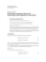
Figure 1: The CPT of a LFM signal.
where φ(t) is the signal phase, b is amplitude, α is initial
frequency, and β is chirp rate. The CPF is defined as
CP(t, u)
=

+∞
0
s(t + τ)s(t −τ)e
−juτ
2
dτ. (2)
By substituting (1)in(2), we obtain
CP(t, u)
= b
2
e
2j(αt+βt
2
)

+∞

0
e
j(2β−u)τ
2
dτ. (3)
Using the identity

+∞
−∞
e
−jmt
2
dt =

π
m
e
−j(π/4)
, m>0, (4)
we obtain


CP(t, u)


=
⎧
⎪
⎪
⎪

⎨
⎪
⎪
⎪
⎩
∞
u = 2β
b
2
2

π
|u − 2β|
u
/
=2β.
(5)
It is not hard to see that CP(t, u) peaks along the curve
u
= 2β, so the chirp rate β can be estimated. Then the
parameters α and b can be estimated by dechirping and
finding the Fourier transform peak. For a discrete signal in
the additive noise
x(n)
= s(n)+v(n), |n|≤
N −1
2
,(6)
where v(n) is complex white Gaussian noise of zero mean
and power of σ

2
. The discrete CPF is defined as
CP(n, u)
=
(N−1)/2

m=0
x(n + m)x(n − m)e
−jum
2
. (7)
The two-dimensional (2D) distribution and three-
dimensional (3D) distribution of the CPF for a LFM signal
are shown in Figures 1(a) and 1(b), respectively. We can see
from Figure 1(a) that the CPF is concentrated along the curve
u
= 2β, and we can obtain the estimation of chirp rate β at
arbitrary time, but from Figure 1(b), we can see that when
n
= 0, the CPF gets its maximum value, hence, the estimation
of

β can be obtained by finding the peak of CP(0, u). Then the
estimation of α and b can be obtained by the following two
expressions:
α = arg max
α






(N−1)/2

n=−(N−1)/2
s(n)e
−j(αn+

βn
2
)





,(8)

b =





1
N
(N−1)/2

n=−(N−1)/2
s(n)e

−j(αn+

βn
2
)





. (9)
The CPF, like the ambiguity function, is bilinear. It, there-
fore, produces “cross-terms” when multiple components are
present. So, the influence of cross-terms should be studied.
Theorem 1. For multicomponent LFM signal, there exist the
“cross-terms” in the CPF, but this w ill not influence the
detection and parameter estimation of the “autoterms.”
Proof. For simplicity, we discuss here the two components
case, which are modeled as
s(t)
= s
1
(t)+s
2
(t) = b
1
e
j(α
1
t+β

1
t
2
)
+ b
2
e
j(α
2
t+β
2
t
2
)
.
(10)
Y. Wang and Y C. Jiang 3
Hence, we obtain
s(t + τ)s(t
−τ)
= b
2
1
e
2j(α
1
t+β
1
t
2

)
e
2jβ
1
τ
2
+ b
2
2
e
2j(α
2
t+β
2
t
2
)
e
2jβ
2
τ
2
+ b
1
b
2
e
j(α
1
+α

2
)t+ j(β
1
+β
2
)t
2
e
j(β
1
+β
2
)τ
2
+j(α
1
−α
2
)τ+2j(β
1
−β
2
)tτ
+ b
1
b
2
e
j(α
1

+α
2
)t+ j(β
1
+β
2
)t
2
e
j(β
1
+β
2
)τ
2
−j(α
1
−α
2
)τ−2j(β
1
−β
2
)tτ.
(11)
The CPF of the “autoterms” has the form of (5), peaks
along the curve u
= 2β
1
and u = 2β

2
,respectively.Nowlet
us compute the CPF of the “cross-terms”
CP
cro
(t, u)
= 2b
1
b
2
e
j(α
1
+α
2
)t+ j(β
1
+β
2
)t
2
×

+∞
0
e
j(β
1
+β
2

−u)τ
2
cos

α
1
−α
2

τ +2

β
1
−β
2

tτ

dτ.
(12)
If u
= β
1
+ β
2
,weobtain


CP
cro

(t, u)


=
2b
1
b
2





+∞
0
cos

α
1
−α
2

τ+2

β
1
−β
2

tτ


dτ




≤




2b
1
b
2

α
1
−α
2

+2

β
1
−β
2

t





< ∞.
(13)
If u
/
=β
1
+ β
2
,weobtain


CP
cro
(t, u)


=
b
1
b
2

π


u −


β
1
+ β
2



. (14)
We can see from (13)and(14) that, the CPF of the
“cross-terms” is bounded, while the CPF of the “autoterms”
is infinite when u
= 2β
1
or u = 2β
2
. So, the existence of
the “cross-terms” does not influence the detection of the
“autoterms.”
Remark 1. The phase information of the LFM signal is
neglected in this paper, because in most situations, the
characteristics of LFM signal are determined by the chirp rate
and initial frequency.
Remark 2. For an LFM signal with finite length, the maxi-
mum value of its CPF is finite, and the result of Theorem 1
is ideal. For a signal in practice, the conclusion above is still
valid.
Remark 3. The CPF algorithm is suitable for the LFM signal
with the constant amplitude, initial frequency, and chirp rate,
which can be illustrated by the definition of the CPF.
Remark 4. The estimate of the chirp rate


β can be obtained
by finding the peak of CP(n, u)in(7) when n
= 0, which
would require O(N) operations. Whereas, the ML algorithm,
the Wigner-Hough transform and the fractional Fourier
transform (FrFt) would require O(N
2
) operations when
estimating the parameters of an LFM signal.
For multicomponent signal, the CLEAN technique [9]
combined with the CPF is proposed to detect the weak
components submerged by the stronger components, just as
follows:
Step 1. Let k
= 1, where k is the number of signal
components, s(t) is the original signal.
Step 2. Compute the CPF of s(t) according to (2), and get its
absolute value
|CP(t, u)|.
Step 3. Finding the peak of
|CP(t, u)|,itisconcentrated
along the curve u
= 2β
k
, then the estimated values
{b
k
, α
k

, β
k
} of the kth LFM component are obtained accord-
ing to (8)and(9).
Step 4. Construct the reference signal s
r1
(t) = exp(−jβ
k
t
2
),
then multiply it with s(t), we obtain s
1
(t) = s(t)s
r1
(t). Now
the kth LFM component has been dechirped to a sinusoidal
signal, while the other components are still LFM signals.
Step 5. Design a filter with narrow bandwidth around α
k
,
then the kth component of s
1
(t) is filtered out and this
operation has little influence on other components.
Step 6. Multiply the residual signal with s
r2
(t) = exp(jβ
k
t

2
),
and the other components can be calibrated to the original
form. So, the residual signal without the kth LFM component
can be obtained.
Step 7. Let k
= k +1,repeatSteps2–6 until the energy of the
residual signal is less than a threshold.
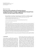
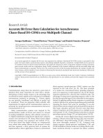
Figure 2 is an example to show the validity of the method
above. There are two LFM components with length 255, the
CPF on the plane (t, u) is shown in Figure 2(a), and the CPF
of the signal that has restrained the first component is shown
in Figure 2(b). We can see that, on the parameter plane,
the weak components will be submerged by the stronger
components, and we can improve the dependability of signal
detection by the CLEAN technique.
3. STATISTICAL PERFORMANCE
3.1. Signal-to-noise ratio
In the presence of signal s(n) without noise, the value
CP
s
(n, u) has a peak at the coordinates (0, 2β); for x(n) =
s(n)+v(n), the value CP
s+v
(n, u) becomes a random variable
and there exists a variance var
{CP
s+v
(0, 2β)}.Theoutput
SNR is defined as

SNR
out
=


CP
s
(0, 2β)


2
var

CP
s+v
(0, 2β)

. (15)
4 EURASIP Journal on Advances in Signal Processing
200
100
0
0
100
200
Relative time
0
500
1000
1500

Amplitude
Relative frequency rate law
(a) The CPF on (t, u)plane
200
100
0
0
100
200
Relative time
0
500
1000
1500
Amplitude
Relative frequency rate law
(b) The CPF of the signal that has restrained the first component
Figure 2: The signal separation based on CLEAN technique.
The expected value of CP
s+v
(0, 2β)is
E

CP
s+v
(0, 2β)

=
(N−1)/2


m=0
E

s(m)s(−m)

e
−2jβm
2
=
1
2
(N +1)b
2
.
(16)
The second-order moment of CP
s+v
(0, 2β)is
E



CP
s+v
(0, 2β)


2

=

(N−1)/2

m=0
(N
−1)/2

k=0
E

s(m)+v(m)

s(−m)+v(−m)
·

s
∗
(k)+v
∗
(k)

s
∗
(−k)+v
∗
(−k)

e
−2jβ(m
2
−k

2
)
=
(N−1)/2

m=0
(N
−1)/2

k=0

s(m)s(−m)s
∗
(k)s
∗
(−k)
+ E

v(m)v
∗
(k)

s(−m)s
∗
(−k)

+ E

v(m)v
∗

(−k)

s(−m)s
∗
(k)
+ E

v(−m)v
∗
(k)

s(m)s
∗
(−k)
+ E

v(−m)v
∗
(−k)

s(m)s
∗
(k)
+ E

v(m)v
∗
(k)

E


v(−m)v
∗
(−k)

+ E

v(m)v
∗
(−k)

E

v(−m)v
∗
(k)

e
−2jβ(m
2
−k
2
)
.
(17)
By computing each term in (17), we obtain
E




CP
s+v
(0, 2β)


2

=

N +1
2

2
b
4
+(N+3)b
2
σ
2
+
N +3
2
σ
4
.
(18)
By combining (16)and(18), we obtain the variance
var

CP

s+v
(0, 2β)

=

N +3

b
2
σ
2
+
N +3
2
σ
4
. (19)
Hence, we can express the output SNR as a function of
the input SNR,
SNR
out
≈
(N/2)SNR
2
in
2SNR
in
+1
, (20)
where SNR

in
= b
2
/σ
2
is the input SNR.
We can see from (20) that at high input SNR (SNR
in

1), the expression (20) can be approximated by SNR
out
=
NSNR
in
/4. Conversely, at low SNR (SNR
in
 1), the expres-
sion (20) can be approximated by SNR
out
= NSNR
2
in
/2, the
output SNR could be even worse than the input SNR. We
can define the threshold of the algorithm as the interception
point between the two limiting behaviors corresponding to
the two cases of high and low SNR, obtaining the SNR
threshold value equal to SNR
in
= 1/2, about −3dB. It is a

constant and the length of signal does not influence the SNR.
Remark 5. Other transformations, such as the fractional
Fourier transform and the Wigner-Hough transform, the
threshold value is 1/N, this is advantageous because the
threshold value can be lowered by increasing the number
of samples [10]. While the threshold of the CPF applied to
LFM signals is a constant, it is disadvantageous. The similar
transformations include the polynomial-phase transform
[11].
3.2. Accuracy
The performance of parameter estimation is usually evalu-
ated by the statistical characteristics of the estimates. Here,
the asymptotic statistical results are derived for all the
estimated parameters based on the first-order perturbation
analysis of maxima of random functions [12]. The following
results can be obtained.
Y. Wang and Y C. Jiang 5
Theorem 2. The mean-square error (MSE) of

β is expressed by
E

(δβ)
2

≈
90
N
5
1

SNR

1+
1
2SNR

. (21)
Theorem 3. The MSE of
α is expressed by
E

(δα)
2

≈
6
N
3
SNR
. (22)
Theorem 4. The MSE of

b is expressed by
E

(δb)
2

≈
σ

2
2N
. (23)
Lemma 1 ([13]). For large N, the Cramer-Rao lower bounds
of β, α,andb are expressed as
CRLB


β

≈
90
SNR·N
5
,
CRLB


α

≈
6
SNR·N
3
,
CRLB


b


≈
σ
2
2N
.
(24)
If we normalize the var iances by the corresponding Cramer-
Rao lower bounds, we obtain the efficiencies
ε
β
≈ 1+
1
2SNR
, ε
α
= ε
b
≈ 1. (25)
Remark 6. The efficiencies of the Wigner-Hough transform
(WHT) is [10]
ε
β
= ε
α
≈ 1+
2
NSNR
+ O

1

N
2

, ε
b
≈ 1. (26)
Compared with the CPF algorithm, the estimate accuracy
of the chirp rate β is higher than the CPF algorithm, and
the estimate accuracy of the initial frequency α and the
amplitude b is the same as the CPF algorithm. But the
implementation of the WHT requires 2D maximizations.
Remark 7. The efficiencies of the fractional Fourier trans-
form (Frft) is [6]
ε
β
= ε
α
≈ 1+
3
2N +1
+ O

1
N
2

, ε
b
≈ 1. (27)
Compared with the CPF algorithm, the estimate accuracy

of the chirp rate β is higher than the CPF algorithm, and
the estimate accuracy of the initial frequency α and the
amplitude b is the same as the CPF algorithm. But the
implementation of the Frft still requires 2D maximizations.
4. SIMULATIONS
In this section, the Monte Carlo simulations are provided to
support the theoretical results. In the experiment, the signal
contains two components, the length of it is 255, and the
parameters of each component are: b
1
= 1, α
1
= π/8, β
1
=
0.005, and b
2
= 0.2, α
2
= π/4, and β
2
= 0.002. The sampling
interval is 1, the value of the input SNR varies from
−4dB
to 11 dB with an interval of 1 dB, we run 200 Monte Carlo
simulations, the measured MSEs (dB) of each parameter and
the theoretical MSEs (dB) just as (21)–(23) are shown in
Figures 3 and 4.
0510
SNR (dB)

−120
−100
−80
−60
MSE(β)
(a)
0510
SNR (dB)
−80
−60
−40
−20
MSE(α)
(b)
0510
SNR (dB)
−40
−30
−20
−10
MSE(b)
(c)
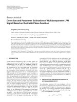
Figure 3: MSEs of parameter estimates of the first component. (Full
lines are the theoretical MSEs, and circles indicate measured MSEs).
As shown in Figure 3, for the first component, when
the SNR is higher than
−2 dB, the measured MSEs and the
theoretical MSEs are well matched. If the SNR is lower than
−2 dB, there exist big errors between the measured MSEs
6 EURASIP Journal on Advances in Signal Processing

0510
SNR (dB)
−120
−100
−80
−60
MSE(β)
(a)
0510
SNR (dB)
−80
−60
−40
−20
MSE(α)
(b)
0510
SNR (dB)
−40
−30
−20
−10
MSE(b)
(c)
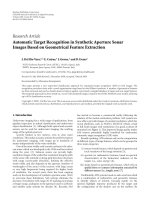
Figure 4: MSEs of parameter estimates of the second component.
(Full lines are the theoretical MSEs, and circles indicate measured
MSEs).
and the theoretical MSEs, this is because the approximations
implied in the theoretical analyses are no longer valid at low
SNRs. For the second component, we can see from Figure 4

that, after filtering out the first component by the CLEAN
technique, the measured MSEs are close to the theoretical
MSEs when the SNR is higher than
−2dB, but compared
with Figure 3, the accuracy decreases in a way, and there
are some irregular variations of the measured MSEs, this is
because of the weakness of the second component compared
with the noise at low SNRs, and the influence of the first
component exists simultaneously.
5. CONCLUSION
The detection and parameters estimation of multicompo-
nent LFM signal can be realized by the CPF. The principle
of detection and parameters estimation of single LFM signal
is presented. For multicomponent LFM signal, the CLEAN
technique combined with the CPF is proposed to detect the
weak components submerged by the stronger components.
The statistical performance is analyzed in this paper and the
simulation results demonstrate the validity of the algorithm
proposed.
REFERENCES
[1] T. J. Abatzoglou, “Fast maximum likelihood joint estimation
of frequency and frequency rate,” IEEE Transactions on
Aerospace and Electronic Systems, vol. 22, no. 6, pp. 708–715,
1986.
[2] R. M. Liang and K. S. Arun, “Parameter estimation for
superimposed chirp signals,” in Proceedings of the IEEE Inter-
national Conference on Acoustics, Speech, and Signal Processing
(ICASSP ’92), vol. 5, pp. 273–276, San Francisco, Calif, USA,
March 1992.
[3] I. Raveh and D. Mendlovic, “New properties of the Radon

transform of the cross Wigner/ambiguity distribution func-
tion,” IEEE Transactions on Signal Processing,vol.47,no.7,pp.
2077–2080, 1999.
[4] Y. Sun and P. Willett, “Hough transform for long chirp
detection,” IEEE Transactions on Aerospace and Electronic
Systems, vol. 38, no. 2, pp. 553–569, 2002.
[5] M. Wang, A. K. Chan, and C. K. Chui, “Linear frequency-
modulated signal detection using Radon-ambiguity trans-
form,” IEEE Transactions on Signal Processing, vol. 46, no. 3,
pp. 571–586, 1998.
[6] L. Qi, R. Tao, S. Zhou, and Y. Wang, “Detection and parameter
estimation of multicomponent LFM signal based on the
fractional Fourier transform,” Science in China Series F, vol.
47, no. 2, pp. 184–198, 2004.
[7] P. O’Shea, “A new technique for instantaneous frequency rate
estimation,” IEEE Signal Processing Letters, vol. 9, no. 8, pp.
251–252, 2002.
[8] P. O’Shea, “A fast algorithm for estimating the parameters of
a quadratic FM signal,” IEEE Transactions on Signal Processing,
vol. 52, no. 2, pp. 385–393, 2004.
[9] J. Tsao and B. D. Steinberg, “Reduction of sidelobe and speckle
artifacts in microwave imaging: the CLEAN technique,” IEEE
Transactions on Antennas and Propagation,vol.36,no.4,pp.
543–556, 1988.
[10] S. Barbarossa, “Analysis of multicomponent LFM signals by
a combined Wigner-Hough transform,” IEEE Transactions on
Signal Processing, vol. 43, no. 6, pp. 1511–1515, 1995.
Y. Wang and Y C. Jiang 7
[11] S. Peleg and B. Porat, “Estimation and classification of
polynomial-phase signals,” IEEE Transactions on Information

Theory, vol. 37, no. 2, pp. 422–430, 1991.
[12] S. Peleg and B. Porat, “Linear FM signal parameter estima-
tion from discrete-time observations,” IEEE Transactions on
Aerospace and Electronic Systems, vol. 27, no. 4, pp. 607–616,
1991.
[13] B. Ristic and B. Boashash, “Comments on “the Cramer-
Rao lower bounds for signals with constant amplitude and
polynomial phase”,” IEEE Transactions on Signal Processing,
vol. 46, no. 6, pp. 1708–1709, 1998.