Báo cáo hóa học: " Research Article A Practical Approach for Simultaneous Estimation of Light Source Position, Scene Structure, and Blind Restoration Using Photometric Observations" pot

Hindawi Publishing Corporation
EURASIP Journal on Advances in Signal Processing
Volume 2008, Article ID 785364, 12 pages
doi:10.1155/2008/785364
Research Article
A Practical Approach for Simultaneous Estimation of
Light Source Position, Scene Struc ture, and Blind Restoration
Using Photometric Observations
Swati Sharma
1, 2
and Manjunath V. Joshi
3
1
Laboratoire d’Imagerie et de Neurosciences Cognitives, UMR CNRS-ULP 7191, 67000 Strasbourg, France
2
Laboratoire des Sciences de l’Image, de l’Informatique et de la T
´
el
´
ed
´
etection, UMR CNRS-ULP 7005, 67412 Illkirch Cedex, France
3
Dhirubhai Ambani Institute of Information and Communication Technology, Gandhinagar 382007, Gujarat, India
Correspondence should be addressed to Swati Sharma,
Received 26 September 2007; Revised 15 February 2008; Accepted 2 April 2008
Recommended by Hubert Cardot
Given blurred observations of a stationary scene captured using a static camera but with different and unknown light source
positions, we estimate the light source positions and scene structure (surface gradients) and perform blind image restoration. The
images are restored using the estimated light source positions, surface gradients, and albedo. The surface of the object is assumed
to be Lambertian. We first propose a simple approach to obtain a rough estimate of the light source position from a single image

using the shading information which does not use any calibration or initialization. We model the prior information for the scene
structure as a separate Markov random field (MRF) with discontinuity preservation, and the blur function is modeled as Gaussian.
A proper regularization approach is then used to estimate the light source position, scene structure, and blur parameter. The
optimization is carried out using the graph cuts approach. The advantage of the proposed approach is that its time complexity is
much less as compared to other approaches that use global optimization techniques such as simulated annealing. Reducing the
time complexity is crucial in many of the practical vision problems. Results of experimentation on both synthetic and real images
are presented.
Copyright © 2008 S. Sharma and ManjunathV. Joshi. This is an open access article distributed under the Creative Commons
Attribution License, which permits unrestricted use, distribution, and reproduction in any medium, provided the original work is
properly cited.
1. INTRODUCTION
Photometric stereo has been used by many researchers for
recovering the shape of the object and the albedo. Here, the
shading cue is used for inferring the shape of the object.
Authors in [1] propose two algorithms for robust shape
estimation for photometric stereo. They combine finite
triangular surface model and the linearized reflectance image
formation model to express the image irradiance. Chen et al.
[2] recover the albedo values for color images using photo-
metric stereo. In [3–5], the authors use a calibrating object
of known shape and constant albedo to establish a nonlinear
mapping between the image irradiance and shape of the
object in the form of a lookup table. For photometric stereo,
a neural network-based approach is presented in [6]fora
rotationally symmetric object with nonuniform reflectance.
Authors in [7] obtain shape from photometric stereo images
with unknown light source positions. However, they do not
attempt to recover the light source positions. Basri et al. [8]
attempt to recover the surface normal in a scene using the
images produced under general lighting condition. They

assume the light sources to be isotropic and distantly located
from the object, assume a combination of point sources,
extended sources, diffused lighting, and represent the general
lighting conditions using low-order spherical harmonics.
In [9], a method to obtain absolute depth from multiple
images based on solving a set of linear equations is proposed.
This method is applicable to a wide range of reflectance
models. Another approach for photometric stereo that is
based on the optical flow is presented in [10]. The input
images are matched through an optical flow and the resulting
disparity field is then used to obtain structure from motion
which does not require the reflectance map information.
Photometric stereo has also been applied to the analysis
2 EURASIP Journal on Advances in Signal Processing
and description of surface structures in [11–14]. It has also
been applied to the problems of machine inspections [15]
and identification of machined surfaces [16]. In [17], graph
cuts minimization technique has been used for estimation
of the surface normals using photometric stereo. They use
the ratio of two images in order to cancel out the albedo in
the image irradiance equation and get the initial estimates
of the surface normal which are required to define the
energy functions. Graph cuts are then used for optimization.
Although, authors in [7, 8] obtain the shape of the object
without the knowledge of the light source position they
do not consider the blur in the observations. In all these
methods, the researchers do not consider the effect of blur
while solving the problem of photometric stereo. In practice,
the observations are often blurred due to camera jitter or out-
of-focus blur. Joshi and Chaudhuri [18] address the problem

of simultaneous estimation of the scene structure and restore
the images considering blurred photometric observations.
They recover the surface gradients and the albedo and also
perform blind image restoration. The surface gradients and
the albedo are modeled as separate Markov random fields
(MRFs), and a suitable regularization scheme is used to
estimate the different fields as well as the blur parameter.
However, they use simulated annealing for optimization
which is very time-consuming and takes hours to reach the
global minima. Also, the light source positions are assumed
to be known. Sharma and Joshi [19]usegraphcutsfor
superresolving the image and scene depth using photometric
cue. However, they do not consider blur on the observations
and use known light source directions. In this paper, we do
not address the superresolution problem, but we estimate
the scene structure, light source position, and perform blind
image restoration.
Most of the researchers, while using shape from shad-
ing and photometric stereo, assume that the light source
positions are known. However, in a practical scenario, the
images are captured without any knowledge of the position
of the light source (with respect to some reference plane).
We now discuss briefly some of the research works that
have been carried out on the estimation of position of the
light source. The problem of obtaining the light source
position from a single image was first addressed in [20]
where the solution is obtained using the derivative of the
image intensity along several directions. The authors in
[21] present two schemes for estimating the illuminant
direction from a single image. One method is based on

local estimates for smooth patches. The second method
uses shading information from image contours. In [22], a
scheme which is based on the concept of critical points
in the image for extracting multiple illuminant directions
from the image of a sphere of known size is proposed. Two
methods for estimating the surface reflectance property of
an object as well as the position of a light source from
a single view without the distant illumination assumption
are proposed in [23]. Given an image and a 3D geometric
model of an object with specular reflection as inputs, the
first method estimates the light source position by fitting
to the Lambertian diffuse component, while separating
the specular and diffuse components by using an iterative
relaxation scheme. The second method extends the first
method by using specular component image as input, which
is acquired by analyzing multiple polarization images taken
from a single view. The authors in [24] combine information
both from the shading of the object and from the shadows
cast on the scene to estimate the position of multiple
illuminants of a scene. In [25], a scheme for locating multiple
light sources and estimating their intensities from a pair of
stereo images of a sphere is discussed. The surface of the
sphere is assumed to have both Lambertian and specular
properties. In [26], a method is presented for calibrating
multiple light source locations in 3D using captured images.
This method uses three spheres at known relative positions
which are used for calibrating the light source directions. In
[27], a fully automatic algorithm for estimating the projected
light source direction from a single image is presented.
The algorithm consists of three stages. First, the potential

occluding contours using color and edge information are
selected, and then for each contour the light source direction
is estimated using a shading model. In the final stage, the
results from the estimations are fused together in a Bayesian
network to arrive at the most likely light source direction.
The approaches proposed in [25, 26] use calibration to find
the light source position, which is a difficult task.
In this paper, we first propose a simple approach for
obtaining the rough estimates of light source position using
a single image. We assume a point light source and one
light source direction for each captured image. We thus
estimate the light source position for each observation in
the photometric stereo setup. It may be mentioned that the
proposed approach for light source direction does not use
any calibration as used by many of the other researchers. We
then estimate the scene structure and the blur parameter and
restore the image. The blur function is modeled as Gaussian
and the surface gradients are modeled as separate Markov
random fields (MRFs) with edge preservation and suitable
regularization is used. A cost function that consists of a
data fitting term and other constraint terms is formulated
and graph cuts approach is used for optimization to get the
final solution. The light source position is also optimized
for each of the captured image. We would like to mention
here that we do not optimize for albedo assuming that it,
as a smooth field and a simple sharpening filter, is used to
remove the effect of blurring from the albedo field. Although
the problem of blind restoration and shape estimation from
blurred photometric observations is solved in [18], they use
known light source positions and do not estimate them

in their formulation. Also, they use simulated annealing
for optimization which is computationally very taxing. In
our formulation, we use graph cuts with proper choice of
label set to considerably reduce the convergence time. It
may be mentioned here that although simulated annealing
yields global minima irrespective of the nature of cost
function, the solution obtained using graph cuts is near
the optimal solution [28] with computational complexity
much less than simulated annealing. In a practical scenario,
time complexity is crucial. For instance, if we consider an
assembly line where an object has to be moved from one
place to another (industrial inspection), the requirement
S. Sharma and ManjunathV. Joshi 3
Object
O(0,0,0)
Image plane
(x
− y plane)
Point light
source
x
y
zn
Camera
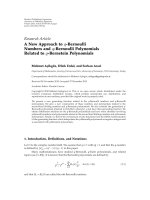
Figure 1: Observation system for photometric stereo.
is to calculate the depth fast enough so that the assembly
line functions smoothly, with a slight compromise on the
high accuracy. In such situations, near global optimization
methods, such as graph cuts, are useful. It is interesting to
note that the rough estimates of the proposed light source

position approach serve as better initial estimates for graph
cuts to reach near optimum result quickly.
It may also be mentioned here that uncalibrated photo-
metric stereo may be used to find the surface gradients and
albedo along with the light source directions and intensities.
However, there is an ambiguity in the estimated values since
these quantities can be determined only up to an arbitrary
invertible matrix [29, 30]. The proposed approach does not
suffer from such a problem. Also, it uses a simple shading
effect which forms the critical boundary in order to obtain
the initial estimate.
The rest of the paper is organized as follows. In Section 2,
we discuss the basic photometric stereo approach for shape
(depth) estimation. Next, we explain the forward model
for formation of blurred images in Section 3. Section 4
describes the proposed approach for light source direction
estimation. A brief overview of the graph cuts optimization
method is presented in Section 5. Section 6 dealswiththe
proposed approach for simultaneous estimation of scene
structure, light source direction, and blind image restoration.
We present the results of experimentation for light source
direction estimation, depth estimation, and blind restoration
of images in Section 7. The paper is concluded with a short
discussion in Section 8.
2. PHOTOMETRIC STEREO
Photometric stereo is a method for estimating the 3D shape
of an object. It requires several images of a stationary object
that are captured using a stationary camera with different
light source positions. Figure 1 shows the observation system
for photometric stereo, in which the object is placed at a

fixed distance from the camera, and the light source is moved
to different positions. For each position of the light source
an image is captured, thus obtaining a set of images as
observations. If a Lambertian surface is assumed, the image
irradiance equation relating the surface gradients and image
intensity can be written as
E(x, y)
= ρ(x, y)n(x, y)·s,
E(x, y)
=
ρ(x, y)

p(x, y)p
s
+ q(x, y)q
s
+1


p(x, y)
2
+ q(x, y)
2
+1

p
2
s
+ q
2

s
+1
,
(1)
where p(x, y), q(x, y) are the surface gradients in x and y
directions, respectively. Here ρ(x, y) represents the albedo,
which is nothing but the fraction of light reflected from
the surface at a point (x, y) and its value lies between
0and1.
n(x, y) denotes the surface normal given by
(
−p(x, y), −q(x, y), 1)/(

p(x, y)
2
+ q(x, y)
2
+1)andE(x, y)
is the image irradiance (or image intensity) at point (x, y)in
the image.
s = (−p
s
, −q
s
,1)/(

p
2
s
+ q

2
s
+ 1) is a unit vector in
the direction of the light source.
The surface gradients and albedo at a point are related
to the intensity at that point according to (1). Since there
are three unknowns p(x, y), q(x, y), ρ(x, y), it is possible
to obtain a unique solution using linearly independent
equations. In real scenario, due to erroneous observations,
the equations may be inconsistent, and hence one needs to
capture more than three images with different light source
positions and obtain the surface gradients and albedo by
solving the overdetermined set of equations using the least
squares (LS) method. Once the surface gradients are known,
an iterative method can be used to obtain the depth map
[31].
3. FORWARD MODEL
Equation (1) relates the true surface gradients and albedo
when we assume that the observations are not blurred.
However, due to the faulty focus settings of the camera, the
observations are often blurred. If the effect of blur and noise
4 EURASIP Journal on Advances in Signal Processing
P(x, y,z)
O(0,0,0)
P(x

, y

, z


)
Image plane
(x
− y plane)
Point light
source (s
x
, s
y
, s
z
)
Object
x
y
z
Figure 2: Experimental setup for estimating illuminant position. P(x, y, z) is a point on the object that is projected onto the image plane at
point P(x

, y

, z

).
is considered, then the image formed for the mth light source
position can be written as [18]
g
m
(x, y) = h(x, y)∗E
m

(x, y)+w
m
(x, y), m = 1, , K,
(2)
where h(x, y) represents the two-dimensional point spread
function (PSF) of the camera, and w
m
(x, y) is the indepen-
dent and identically distributed (i.i.d) additive noise, and
K denotes the number of blurred observations considered.
Since, there is no relative motion between the camera and
the object, the PSF remains same for all the observations.
We also assume that the blur is space-invariant, and hence
a single blur mask is assumed for the entire observed image.
We also assume that there is no chromatic aberration due to
the camera lens.
Now, let E
m
be a vector containing the unblurred
intensity values of the mth image of size M
× N arranged
in lexicographical order. E
m
is a function of ρ, p, q,ands
m
which are the true values of the surface gradients, albedo, and
the light source position. If g
m
represents the corresponding
observation vector, (2)canbewrittenas

g
m
= H(σ)E
m

ρ, p, q, s
m

+ w
m
, m = 1, , K,(3)
where H(σ) is the MN
× MN matrix and σ is the blur
parameter. The blur is assumed to be due to the fact that the
camera is out of focus. This can be modeled by a pillbox blur
or by a Gaussian PSF characterized by the parameter σ [32].
In our work, we assume Gaussian PSF with blur parameter
σ. Now, the problem is to estimate the light source positions,
the surface gradients, the albedo, and blur parameter given
the observations. This is definitely an ill-posed problem and
it requires the use of regularization to obtain better estimates.
While solving for the surface gradients and albedo using
(1), one needs to know the light source direction. In a
practical scenario, these are not known. In the following
section, we discuss a simple approach for obtaining rough
estimates of light source positions.
4. PROPOSED APPROACH FOR INITIAL ESTIMATES OF
LIGHT SOURCE POSITIONS
Here, we discuss a simple shading-based method that uses
the position of the critical boundary formed on the image of

the object being imaged to estimate the light source position.
The critical boundary is defined as that boundary beyond
which the imaged object is not visible in the image due to the
position of the light source. We assume that there is no self-
occlusion and such a boundary exists due to the light source
position. A single light source position is estimated for each
of the blurred observations. We assume a point light source
and an orthographic projection is assumed eliminating the
need for geometric correction.
In this section, we use a different convention to represent
the light source positions. The light source position is
estimated with respect to a coordinate system. Let the vector
(s
x
, s
y
, s
z
) represent the true light source position in the
coordinate system. In the notation used in Section 2, the unit
light source vector is represented as (
−p
s
, −q
s
,1). Thus, we
have the relation
p
s


p
2
s
+ q
2
s
+1
=
−
s
x

s
2
x
+ s
2
y
+ s
2
z
,
q
s

p
2
s
+ q
2

s
+1
=
−
s
y

s
2
x
+ s
2
y
+ s
2
z
,
1

p
2
s
+ q
2
s
+1
=
s
z


s
2
x
+ s
2
y
+ s
2
z
.
(4)
S. Sharma and ManjunathV. Joshi 5
Figure 2 shows the position of the camera, the object, and
the light source with respect to the coordinate system. Both
the camera and the light source are placed in front of the
object. We use simple geometry to find the light source
position. The shading-based method for estimating the light
source position is based on the fact that the critical boundary
moves whenever the position of the light source changes.
At the critical boundary on the image plane, a ray of light
emanating from the light source becomes tangential (as the
object is not visible in the image beyond that boundary).
We refer to the coordinates of the image points on the
end points of the critical boundary as critical points. If the
critical points are known, then the tangents drawn at those
points intersect at the point where the point light source
is located. We use a simple binary thresholding followed
by edge detection to obtain the critical boundary. Figure 3
illustrates the geometry used for the proposed method. The
figure shows the tangents on the critical boundary and the

light source position, given by the intersection of the tangents
to the circle at the critical points. The dark portion of the
figure shows the portion of the object beyond the critical
boundary, which is not visible in the image. The light sources
thus estimated for each observation are refined using the
graph cuts optimization. It may be noted that we obtain the
light source position using geometry on the image which
lies on the x
− y plane, only the x and y coordinates of the
light source direction can be estimated using our approach.
The obtained coordinates are normalized to get the direction
vector. We represent these as s

x
and s

y
. The shading-based
method can be summarized as follows.
(1) The given image is thresholded into two regions,
depending on whether the portion of the object
being imaged is visible in the image or not. We use
the “watershed” function available in MATLAB to
segment the object from the background.
(2) Edges are extracted from the image to get the critical
boundary.
(3) Next, a best fit circle in the least square sense is
estimated using the points on the critical boundary.
(4) Two tangents are drawn, one on each of the critical
points of the critical boundary.

(5) The point of intersection of these tangents gives x and
y coordinates of the light source position.
The rough estimates of the light source positions obtained
from the blurred observations are used to obtain the initial
values of p, q,andρ (using the least squares method as
mentioned in Section 2), thus ensuring better initial esti-
mates that aid in the quick convergence of the optimization
using graph cuts. However, while using (1) to find the surface
gradients and albedo, the z coordinate of the light source
position is initialized as follows. A small value ε is subtracted
from s

x
and s

y
such that the relation (s

x
− ε)
2
+(s

y
− ε)
2
+
s
2
z

= 1 is satisfied. We subtract a small value ε from the values
s

x
and s

y
(estimated geometrically from the image) as these
values are already close to the true values. Since s

x
and s

y
are
already normalized and close to the normalized true values
Light source
position
Critical point 1
Critical point 2
Ta ng e nt 1
Ta ng e nt 2
Critical boundary
c
Figure 3: Illustration of the geometry used by the method. Also,
shown are tangents on the critical boundary and the light source
position (as the intersection of the two tangents at the critical
points).
s
x

/(

s
2
x
+ s
2
y
+ s
2
z
)ands
y
/(

s
2
x
+ s
2
y
+ s
2
z
),thisstepisrequired
so that the estimated initial light source position becomes a
valid direction.
5. INTRODUCTION TO GRAPH CUTS
Many researchers use global optimization techniques such as
simulated annealing for minimization of energy functions.

Although, simulated annealing is theoretically capable of
finding the global minima of an arbitrary energy function,
it is computationally very expensive and hence practically
not feasible. Recently, algorithms have been proposed for
optimization using graph cuts which guarantee that the
solution obtained either reaches the global optimum or
reaches local minima close to the global minimum [28]quite
fast.
One of the most widely used energy function in the graph
cuts framework is as follows [28]:
E( f )
=

(x,y)∈S
Data

f (x, y)

+

(x,y),(u,v)∈N
V
(x,y),(u,v)

f (x, y), f (u,v)

.
(5)
Data( f (x, y)) is a function derived from the observed
data that measures the cost of assigning the label f (x, y)

to the pixel (x, y)
∈ S, S being the image grid. The
label may represent an image intensity for a restoration
problem or may be a surface gradient while estimating shape.
V
(x,y),(u,v)
( f (x, y), f (u, v)) is the term used to incorporate
the spatial smoothness. This measures the cost of assigning
the labels f (x, y)and f (u, v) to two adjacent pixels at (x, y)
and (u,v). This is also the typical energy function that uses
MRF modeling. Graph cuts can be used for minimization
of only a certain type of energy functions. Minimization
via graph cuts is possible only if the cost function is graph
representable. It has been proved that an energy function
is graph representable provided the energy function satisfies
the regularity condition [33].
Minimization of an energy function by graph cuts is
basically finding that cut on the graph which has the min-
imum cost. Such algorithms are called min-cut/max-flow
6 EURASIP Journal on Advances in Signal Processing
algorithms. Global minimization of these energy functions
is NP-hard even in the simplest discontinuity-preserving
case. In [28], two min-cut/max-flow algorithms, α
− β swap
and α expansion have been proposed. It has been proved
that iteratively running the expansion algorithm produces
approximate solutions within a factor of two of the global
minima for a multilabel case provided that the smoothness
term V
(x,y),(u,v)

( f (x, y), f (u, v)) is a metric. This motivates us
to use graph cuts as an optimization method in our work.
6. ESTIMATION OF SCENE STRUCTURE, LIGHT
SOURCE POSITION, AND BLIND RESTORATION
In the following section, we explain how we solve our
problem of estimating the light source directions, surface
gradients, and the blur parameter.
6.1. Data fitting term
Since, we have many observations of the same stationary
object captured with a stationary camera, the data fitting
term (from (3)) can be written as
Dataterm
=
K−1

m=0


g
m
− H(σ)E
m

ρ, p, q, s
m



2
,(6)

where the symbols have their usual meaning. In this case,
the variables are surface gradients, that is, p(x, y)and
q(x, y), albedo ρ(x, y) at every pixel (x, y) of the image.
Also, the illuminant position
s
m
is unknown but is the same
for the entire image. In order to simplify calculations, we
parameterize the point light source in terms of the tilt (τ
m
)
and slant (γ
m
) angles. Then, the unit vector in the illuminant
direction is
s
m
=

s
x
m
, s
y
m
, s
z
m

=


cos

τ
m

sin

γ
m

,sin

τ
m

sin

γ
m

,cos

γ
m

.
(7)
This a multilabel minimization problem with a number of
unknowns.

The energy function should satisfy the regularity con-
dition so that it can be minimized using graph cuts
formulation. Applications of graph cuts generally use the
data term that is a function of a single pixel [34] since a
function of a single variable is always regular [33].
Consider the data fitting term for a particular pixel (x, y)
of the images. Equation (6)canbewrittenas
Dataterm(x, y)
=
K−1

m=0

g
m
(x, y)−
u

i=−u
v

j=−v
h(i, j)F
m
(x, y)

2
,
(8)
where

F
m
(x, y)=E
m

ρ(x−i, y−j), p(x−i, y−j), q(x−i, y−j), s
m

,
(9)
where h is an S
× T blurring mask, u = (S − 1)/2, and
v
= (T −1)/2. Since the blurring function H(σ)operateson
more than one pixel, the data term is not regular. In order to
use the graph cuts formulation, we apply valid mathematical
approximations to the data fitting term such that the data
term becomes a function of a single pixel. For each pixel
(x, y), we consider the terms not depending on (x, y)as
constant for a particular optimization step. Then (8)canbe
rewritten as
Dataterm(x, y)
=
K−1

m=0

g
m
(x, y) −


h(0, 0)F
m
(x, y)+C

2
,
(10)
C
=
u

i=−u
v

j=−v
h(i, j)F
m
(x, y), i
/
=0, j
/
=0. (11)
6.2. Prior modeling
We model the prior information of the surface gradients as
separate Markov random fields (MRFs). By using the MRF
prior, the spatial dependency between the neighboring pixels
can be easily accounted. Generally, the depth variation of an
object is smooth with occasional discontinuities representing
sudden change in depth. We capture this relationship by

using the smoothness term with discontinuity preservation
for edges. In this case, a truncated linear prior as defined
in [28] is used. The discontinuity preservation depends on
the choice of parameter T. This prior is piecewise smooth,
and hence it ensures that the solution does not become over
smooth, and discontinuities are preserved. The smoothness
term for two neighboring pixels (x, y)and(k, l)isgivenby
the following expression:
V
(x,y),(k,l)

f (x, y), f (k, l)

=
min



f (x, y) − f (k,l)


, T

,
(12)
where T is a positive constant. The smoothness term satisfies
the regularity condition if it is a metric. It can be easily
verified that (12) satisfies the conditions of a metric. Here,
f (x, y) is the label assigned to the pixel (x, y). So, f (x, y)can
be either p(x, y)orq(x, y). We use the following truncated

linear prior for p and q:
U(t)
= λ
t
M

x=1
N

y=1

min

t(x, y) −t(x − 1, y), T
t

+min

t(x, y) −t(x, y − 1), T
t

,
(13)
where t = p or q.
6.3. Source position direction constraint
Since we estimate the normalized light source direction, the
estimated value of the illuminant position should satisfy
||s||
2
= 1, (14)

where s
= (s
x
, s
y
, s
z
). This ensures that the light source
position is a unit vector in the direction of the source.
This constraint is used while optimizing to ensure better
convergence of the light source positions.
S. Sharma and ManjunathV. Joshi 7
6.4. Total cost function
Since we use a regularization-based approach, the total cost
function can be obtained by combining the data term,
smoothness term, and the source position constraint. Thus
using (10), (13), and (14), we can express the total cost
function as
ε
=
K−1

m=0

over all x;y

g
m
(x, y)
−


h(0, 0)E
m

ρ(x, y), p(x, y), q(x, y), s
m

+ C

2
+ U(p)+U(q)+

s
2
− 1

2
.
(15)
In our implementation, we optimize one variable at a
time keeping the others constant. For example, the cost
is minimized first using p values, keeping the values of
q, τ
m
, γ
m
,andσ constant. Using the optimized values of p,
we minimize for q, keeping the other variables unchanged.
This is repeated in each cycle for all the variables until
convergence is reached. It may be mentioned here that p, q

are all matrices. γ
m
and τ
m
are real values corresponding
to a particular source position and σ is also a real value.
As already mentioned, we use the albedo values that are
unblurred using a simple high pass filter to reconstruct the
restored images for each light source direction. The depth is
estimated using the estimated p and q values [31].
6.5. Choice of the label set
Graph cuts require a discrete label set. Many of the pro-
posed methods use graph cuts because optimization use
integer labels, for example, see [35]. In our case, we use
discrete floating point labels. Knowing the initial light source
position estimates, one can obtain the initial estimates for
p, q, and albedo using an LS approach. Based on the
frequency distribution (histogram) of p and q labels, it is
possible to quantize the entire range of continuous labels
in a nonuniform fashion to get a discrete label set. The
nonuniform quantization is done so that maximum number
of labels (discrete and integer) is assigned to that subrange
which has a higher probability. For τ and γ, the set of labels
is selected by trial and error around the initially obtained
values. The number of labels, in this case, is directly related
to the precision. As the chosen number of labels is increased,
more accurate estimates may be obtained with a slight
increase in computational complexity.
7. EXPERIMENTAL RESULTS
In this section, we present some of our experimental results

for the proposed approach to recover the light source
positions, depth estimation (using the estimated surface
gradients), and blind restoration. Experimental results are
shown for synthetically generated images as well as for real
images.
(a) (b)
Figure 4: (a) Synthetically generated hemisphere image with light
source position (0.1545, 0.9755, 0.1564) and (b) the corresponding
edge image.
7.1. Experimental results on initial estimates of
light source positions
We first consider the experimentation for estimating the light
source position using the proposed shading-based method.
An image of a hemisphere with known light source position
is synthesized. While conducting the experiment, we assume
that the light source position is unknown. Figure 4(a) shows
the image of the hemisphere with normalized x and y
coordinates of the light source direction as (0.1545, 0.9755),
and the corresponding edge image is shown in Figure 4(b).
We use a simple canny edge detection technique to obtain
the edge image. Since the image is a circle, the line joining the
center of the image to the critical points will be perpendicular
to the tangents at these points, and the intersection point
of these tangents gives the x and y coordinates of the
light source position. The estimated values of the x and
y coordinates of light source position in this case are
(0.1592, 0.9872) which are quite close to the true estimate.
Ta ble 1 shows the actual and estimated values of x and y
coordinates of the light source direction for the images of the
hemisphere generated using different light source directions.

We next consider a real image with unknown light source
directions where the critical boundary may not be a smooth
curve. Figure 5(a) shows the image of a soft toy “Jodu”
captured with some unknown light source position and the
corresponding edge image is shown in Figure 5(b). In this
case, in order to obtain the light source position, we fit a circle
through the image points that lie on the critical boundary.
Now, the two critical points are selected on this circle, and
the point of intersection of the tangents at these points is the
light source position. This experiment was repeated on a set
of eight images of Jodu so that they can be used as the initial
estimates for graph cuts optimization. In order to verify the
correctness of the light source direction, we reconstruct the
images using these estimated light source positions and the
initial estimates of p, q,andρ obtained using them (refer
to (1)). The reconstructed image displayed in Figure 5(c) has
been shading very close to the displayed image in Figure 5(a).
This indicates that these initial estimates of the light source
position when further used in graph cuts optimization lead
8 EURASIP Journal on Advances in Signal Processing
(a)
Critical
point
Critical
boundary
Light
source
position
(b) (c)
Figure 5: (a) Observed Jodu image with unknown light source position. (b) Edge image of Jodu with the same source position. Also shown in

the figure is the circle fitted for the critical boundary and the light source position. (c) Reconstructed Jodu image with the initially estimated
light source direction (0.3821,0.7035, 0.5992).
Table 1: Actual and estimated values of x and y coordinates of the
light source position for the hemisphere image.
Actual source position Estimated source position
xy x y
0.1545 0.9755 0.1592 0.9872
0.2034 0.9568 0.2069 0.9874
0.3716 0.8346 0.4172 0.9088
0.2939 0.9045 0.2916 0.9566
to convergence of the x, y,andz coordinates of the light
source positions.
7.2. Experimental results on depth estimation and
blind restoration of images
In order to obtain the depth map and blind restoration
of images, we need to estimate the surface gradients and
the blur parameter given the blurred observations. Since
the initial light source positions are already known, we
obtain the initial p, q,andρ values which serve as initial
estimates for optimization. As mentioned earlier, we do not
optimize the albedo field. For the implementation, we use
the graph cuts library provided by Kolmogorov [28, 33, 36].
Particularly, we use the expansion algorithm for the cost
function minimization. As already discussed, we use a fixed
set of labels for each of the entities p, q, light source position,
and the blur parameter.
We first consider a synthetic image of a vase with a
checkerboardpatternonit.Eightimageseachofsize128
×
128 are generated with different light source positions using

a computer program. In order to test our algorithm, we
blur the vase images using a Gaussian blur kernel since
the blur due to defocus can be modeled as Gaussian [32].
However, we assume that the blur is space invariant for
our experiments. Since the defocus is assumed to be small,
the blur parameter (σ) of the Gaussian function is assumed
to lie in the range (0.5, 1.5). For this experiment, the blur
(a) (b)
Figure 6: Synthesized vase images with source positions: (a)
(0.2995, 0.4827, 0.8230), (b) (0.4379, 0.4827, 0.7585).
(a) (b)
Figure 7: Restored vase images using the proposed approach for the
observations in Figure 6. The estimated light source positions are
(0.3871, 0.5492, 0.7407) and (0.4554, 0.3778, 0.8062), respectively.
parameter was chosen to be σ = 1 and the kernel size was 7×
7. Figure 6 shows two of the observed vase images with true
light source positions: Figure 6(a) (0.2995, 0.4827, 0.8230)
and Figure 6(b) (0.4379, 0.4827, 0.7585). The blur parameter
σ estimated using our approach is 0.93whichisveryclose
to the true value of σ
= 1. The number of labels for
estimating the same was chosen as 10. Figures 7(a) and
S. Sharma and ManjunathV. Joshi 9
(a) (b) (c)
Figure 8: Depth map for vase (a) ground truth and obtained using (b) LS approach on blurred images and (c) proposed approach.
7(b) show the restored vase images after optimization with
graph cuts. The two images have similar shading as given
in Figures 6(a) and 6(b) indicating that the source positions
estimated are close to the correct values. The sharp square
patches with clear edge detail indicate that the images are well

restored. Figures 8(a) and 8(b) show the ground truth for
depth and that obtained using blurred images. The ground
truth for the vase image is known since it is a synthetic
image. Figure 8(c) displays the recovered depth map using
the proposed approach. The depth map is shown as an
intensity image that represents the depth values scaled in the
range 0–255. The scaling is done such that higher intensity
pixels in the depth map represent points closer to the camera
in the object.
For the vase image, we observed that the initial values of
p and q lie in the range (
−4, 0.6) and (−0.2, 0.3), respectively.
Hence, depending on the frequency distributions of the
respective entities, we used 388 and 350 labels for p and q,
respectively. The number of labels for both the tilt and slant
angles of the light source position were chosen as 40. The
regularization parameters λ
p
and λ
q
for p and q fields (in
(13)) were manually selected as 0.075 and 0.034, respectively.
The value of T
t
of the truncated linear prior was chosen to be
0.175. These were chosen on a trial and error basis.
In order to test our algorithm on real images, we next
consider the experimentation on two real image sets, Jodu
and shoe. The light source positions are unknown for Jodu
images but the same is available for shoe images. We slightly

defocus the camera setting to obtain the blurred Jodu and
shoe observations. In a real scenario, this is due to improper
focus setting while using an inferior quality camera.
We first consider Jodu images. Two of the observed
images, with unknown light source positions, are shown in
Figures 9(a) and 9(b). Figures 10(a) and 10(b) show the
restored Jodu images after optimization using our approach.
In both cases, it can be clearly seen that the two images have
been shading very similar to that displayed in Figures 9(a)
and 9(b), indicating that the estimated source positions are
close to the true values. The reconstructed images are also
sharper as compared to the blurred observations indicating
that they are restored well. The blur parameter σ estimated
for this experiment was 0.84.
(a) (b)
Figure 9: Observed Jodu images with unknown light source
directions.
(a) (b)
Figure 10: Reconstructed Jodu images after optimization using
graph cuts. In this case, the estimated source positions are (a)
(0.4379, 0.4827, 0.7585), (b) (
−0.5428, −0.4823, 0.6875).
The initialization for this experiment was kept as follows.
Since the initial values of p were in the range (
−1, 1) and that
for q lies in the range (
−0.6, 0.6), depending on the frequency
distributions of the respective entities, we used 440 and 420
labels for p and q, respectively. The other parameters λ
t

and
T
t
,wheret = p, q, as well as the number of labels for tilt
and slant angles of the light source position and the blur
parameters were kept the same as the previous experiment,
for both Jodu and shoe image sets.
10 EURASIP Journal on Advances in Signal Processing
(a) (b)
Figure 11: Observed shoe images with true light source directions
(a) (0.6736, 0.3042, 0.6736), (b) (
−0.6123, −0.3042, 0.7297).
(a) (b)
Figure 12: Reconstructed shoe images after optimization using
graph cuts. In this case, the estimated source positions are (a)
(0.5567, 0.1250, 0.8213), (b) (0.4215,
−0.2340, 0.8761).
Two of the observed shoe images, with known light
source positions, are shown in Figures 11(a) and 11(b).
Figures 12(a) and 12(b) show the restored shoe images after
optimization using our approach. In this case, although
the estimated images look sharper than that displayed in
Figures 11(a) and 11(b), the shading differs. This is due to
the absence of a clear critical boundary in the shoe images,
which degrades the performance of our light source position
estimation algorithm. The blur parameter σ estimated for
this experiment was 0.95. For this experiment, the initial
values of p and q were in the range (
−4, 9) (440 labels) and
(

−7, 6) (440 labels), respectively.
We now show the performance of our approach for depth
estimation. Figures 13(a) and 13(b) show the depth maps
for Jodu image obtained from blurred Jodu images using
LS approach and that obtained using our graph cuts-based
approach. One can observe that the discontinuities are better
preserved in Figure 13(b), which can be clearly seen in the
portion near Jodu’s eyes, mouth, and nose. Figures 14(a) and
14(b) show the depth maps for shoe image obtained from
blurred shoe images using LS approach and that obtained
using our graph cuts-based approach. Here, the shoe was
kept at angle with the image plane and this causes linear
intensity variation in the depth map. This can be observed
in Figure 14(b) indicating a better depth estimate.
Table 2: PSNR comparison for vase images. The (depth) row in the
table gives the PSNR comparison for the depth field.
True PSNR in dB
source position Blurred images Graph cuts
Vase image
(0.438, 0.483, 0.759) 55.22 55.75
(0.2995, 0.4827, 0.8230) 54.97 55.33
(Depth) 77.30 76.62
(a) (b)
Figure 13: Depth map for Jodu obtained using (a) LS approach on
blurred images, (b) proposed approach.
In order to compare the performance based on the
quantitative measure, we use peak signal-to-noise ratio
(PSNR) as a figure of merit for both the reconstructed images
and the depth map. The expression for PSNR is given as
follows:

PSNR
= 20 log

255
√
MSE

, (16)
where
MSE
=
1
MN
M−1

x=0
N
−1

y=0

I(x, y) −J(x, y)

2
(17)
for two M
×N images I and J.HereI is the true image and J
represents either the observed blurred image or the estimated
one.
Ta ble 2 shows the PSNR values for the blurred vase

images and those obtained after using the proposed
approach. The values are tabulated for vase intensity image
with two different light source positions as well as for the
depth. We can clearly see that with the graph cuts-based
approach the PSNR improves for the restored images.
Since vase is a smooth image, the depth map recon-
structed from the blurred images using the correct light
source positions is close to the ground truth. Hence in case of
the reconstructed depth map using the proposed approach,
there is a slight decrease in the value of PSNR although
perceptually it is close to the ground truth as is clearly seen
in Figure 8(c). It may be mentioned here that we cannot
compare PSNR for the restored Jodu and shoe images as well
as their depth maps, since we do not have the ground truth.
We would also like to mention that our method works
well for sphere-shaped objects (for, e.g., vase image) as the
S. Sharma and ManjunathV. Joshi 11
(a) (b)
Figure 14: Depth map for shoe obtained using (a) LS approach on
blurred images, (b) proposed approach.
method relies on fitting a circle on the critical boundary.
However, in our experiments on arbitrary object shapes
(Jodu and shoe), we found no convergence problems when
we used the light source positions estimated using the
proposed approach as initial estimates and then refined them
using graph cuts.
We now compare the time complexity of our approach
with that proposed in [18], where simulated annealing is
used for optimization in order to preserve the disconti-
nuities. The convergence time for the algorithm proposed

in the paper was of the order of hours which makes the
algorithm unfit in a practical scenario. Our approach, on the
other hand, takes around 5–7 minutes for convergence. All
experiments were performed on a 1.33 GHz processor usin
vase, Jodu, and shoe images of size 128
×128, 234×234, and
265
× 265, respectively.
8. CONCLUSIONS
In this paper, we present a practical approach for photomet-
ric stereo. First, we propose a simple method to obtain rough
estimates for light source position which does not require
any calibration or initialization. We then use these initial
estimates to obtain the light source positions, blur parameter,
scene depth, as well as the restored images given only the
blurred photometric observations. A proper regularization
scheme is used for the same, and graph cuts were used for
optimization. The advantage of the proposed approach is
that we obtain the light source position, scene structure,
and perform blind restoration given just the observations.
The results show that the proposed approach produces
results close to the desired solution. Results also show that
the proposed approach is very fast as compared to other
approaches that use global optimization techniques like
simulated annealing. Thus our approach is useful in practical
applications where computation time is a constraint.
ACKNOWLEDGMENTS
The authors would like to thank the reviewers for their
constructive suggestions and comments. They also would
like to thank Dr. Andr

´
e Jalobeanu, LSIIT, Universit
´
eLouis
Pasteur (Illkirch, France), for his suggestions on improving
the initial draft.
REFERENCES
[1] K. M. Lee and C C. J. Kuo, “Shape reconstruction from
photometric stereo,” in Proceedings of IEEE Computer Society
Conference on Computer Vision and Pattern Recognition (CVPR
’92), pp. 479–484, Champaign, Ill, USA, June 1992.
[2] C Y. Chen, R. Klette, and R. Kakarala, “Albedo recovery
using photometric stereo approach,” in Proceedings of the 16th
International Conference on Pattern Recognition (ICPR ’02),
vol. 3, pp. 700–703, Quebec, Canada, August 2002.
[3] Y. Iwahori, R. J. Woodham, M. Ozaki, H. Tanaka, and
N. Ishii, “Neural network based photometric stereo with a
nearby rotational moving light source,” IEICE Transactions on
Information and Systems, vol. E80-D, no. 9, pp. 948–957, 1997.
[4] Y. Iwahori, R. J. Woodham, and A. Bagheri, “Principal
component analysis and neural network implementation of
photometric stereo,” in Proceedings of the Workshop on Physics-
Based Modeling in Computer Vision, pp. 117–125, Cambridge,
Mass, USA, June 1995.
[5] R. J. Woodham, “Gradient and curvature from the
photometric-stereo method including local confidence
estimation,” Journal of the Optical Society of America A, vol.
11, no. 11, pp. 3050–3068, 1994.
[6] Y. Iwahori, R. J. Woodham, Y. Watanabe, and A. Iwata, “Self-
calibration and neural network implementation of photomet-

ric stereo,” in Proceedings of the 16th International Conference
on Pattern Recognition (ICPR ’02), vol. 4, pp. 359–362, Quebec,
Canada, August 2002.
[7] O. Drbohlav and R. Sara, “Unambiguous determination of
shape from photometric stereo with unknown light sources,”
in Proceedings of the 8th IEEE International Conference on
Computer Vision (ICCV ’01), vol. 1, pp. 581–586, Vancouver,
Canada, July 2001.
[8] R.Basri,D.Jacobs,andI.Kemelmacher,“Photometricstereo
with general, unknown lighting,” International Journal of
Computer Vision, vol. 72, no. 3, pp. 239–257, 2007.
[9] J.J.Clark,“Activephotometricstereo,”inProceedings of IEEE
Computer Society Conference on Computer Vision and Pattern
Recognition (CVPR ’92), pp. 29–34, Champaign, Ill, USA, June
1992.
[10] J. R. A. Torre
˜
ao, “A new approach to photometric stereo,”
Pattern Recognition Letters, vol. 20, no. 5, pp. 535–540, 1999.
[11] G. McGunnigle and M. J. Chantler, “Rotation invariant
classification of rough surfaces,” IEE Proceedings: Vision, Image
and Signal Processing, vol. 146, no. 6, pp. 345–352, 1999.
[12] G. McGunnigle and M. J. Chantler, “Rough surface classifica-
tion using point statistics from photometric stereo,” Pattern
Recognition Letters, vol. 21, no. 6-7, pp. 593–604, 2000.
[13] G. McGunnigle and M. J. Chantler, “Modelling deposition of
surface texture,” Electronics Letters, vol. 37, no. 12, pp. 749–
750, 2001.
[14] M. L. Smith, G. Smith, and T. Hill, “Gradient space analysis
of surface defects using a photometric stereo derived bump

map,” Image and Vision Computing, vol. 17, no. 3-4, pp. 321–
332, 1999.
[15] P. Hansson and P. Johansson, “Topography and reflectance
analysis of paper surfaces using a photometric stereo method,”
Optical Engineer ing, vol. 39, no. 9, pp. 2555–2561, 2000.
12 EURASIP Journal on Advances in Signal Processing
[16] G. McGunnigle and M. J. Chantler, “Segmentation of
machined surfaces,” in Proceedings of the Irish Machine Vision
and Image Processing Conference (IMVIP ’01), pp. 200–207,
Maynooth, Ireland, September 2001.
[17] T P. Wu and C K. Tang, “Dense photometric stereo using
a mirror sphere and graph cut,” in Proceedings of the IEEE
Computer Society Conference on Computer Vision and Pattern
Recognition (CVPR ’05), vol. 1, pp. 140–147, San Diego, Calif,
USA, June 2005.
[18] M. V. Joshi and S. Chaudhuri, “Joint blind restoration and
surface recovery in photometric stereo,” JournaloftheOptical
Society of America A, vol. 22, no. 6, pp. 1066–1076, 2005.
[19] S. Sharma and M. V. Joshi, “A practical approach for super-
resolution using photometric stereo and graph cuts,” in
Proceedings of the 18th British Machine Vision Conference
(BMVC ’07), Warwick, UK, September 2007.
[20] A. P. Pentland, “Finding the illuminant direction,” Journal of
the Optical Society of America, vol. 72, no. 4, pp. 448–455, 1982.
[21] Q. Zheng and R. Chellappa, “Estimation of illuminant
direction, albedo, and shape from shading,” IEEE Transactions
on Pattern Analysis and Machine Intelligence,vol.13,no.7,pp.
680–702, 1991.
[22] Y. Zhang and Y H. Yang, “Illuminant direction determination
for multiple light sources,” in Proceedings of the IEEE Computer

Society Conference on Computer Vision and Pattern Recognition
(CVPR ’00), vol. 1, pp. 269–276, Hilton Head Island, SC, USA,
June 2000.
[23] K. Hara, K. Nishino, and K. Ikeuchi, “Light source position
and reflectance estimation from a single view without the dis-
tant illumination assumption,” IEEE Transactions on Pattern
Analysis and Machine Intelligence, vol. 27, no. 4, pp. 493–505,
2005.
[24] Y. Wang and D. Samaras, “Estimation of multiple directional
light sources for synthesis of mixed reality images,” in
Proceedings of the 10th Pacific Conference on Computer Graphics
and Applications (PCCGA ’02), pp. 38–47, Beijing, China,
October 2002.
[25] W. Zhou and C. Kambhamettu, “Estimation of the size and
location of multiple area light sources,” in Proceedings of the
17th International Conference on Pattern Recognition (ICPR
’04), vol. 3, pp. 214–217, Cambridge, Mass, USA, August 2004.
[26] M.W.Powell,S.Sarkar,andD.Goldgof,“Asimplestrategyfor
calibrating the geometry of light sources,” IEEE Transactions
on Pattern Analysis and Machine Intelligence,vol.23,no.9,pp.
1022–1027, 2001.
[27] P. Nillius and J O. Eklundh, “Automatic estimation of the
projected light source direction,” in Proceedings of the IEEE
Computer Society Conference on Computer Vision and Pattern
Recognition (CVPR ’01), vol. 1, pp. 1076–1083, Kauai, Hawaii,
USA, December 2001.
[28] Y. Boykov, O. Veksler, and R. Zabih, “Fast approximate energy
minimization via graph cuts,” IEEE Transactions on Pattern
Analysis and Machine Intelligence, vol. 23, no. 11, pp. 1222–
1239, 2001.

[29] H. Kong, P. Xu, and E K. Teoh, “Binocular uncalibrated
photometric stereo,” in Proceedings of the 2nd International
Symposium on Advances in Visual Computing (ISVC ’06), vol.
4291 of Lecture Notes in Computer Science, pp. 283–292, Lake
Tahoe, Nev, USA, November 2006.
[30] H. Kong, E K. Teoh, J G. Wang, and R. Venkateswarlu,
“Coplanar light sweep-surface supported uncalibrated pho-
tometric stereo,” in Proceedings of the 17th International
Conference on Pattern Recognition (ICPR ’04), vol. 4, pp. 92–
95, Cambridge, Mass, USA, August 2004.
[31] B. K. P. Horn, Robot Vision, MIT Press, Cambridge, Mass,
USA, 1986.
[32] S. Chaudhuri and A. N. Rajagopalan, DepthfromDefocus:
A Real Aperture Imaging Approach,Springer,NewYork,NY,
USA, 1999.
[33] V. Kolmogorov and R. Zabih, “What energy functions can
be minimized via graph cuts?” IEEE Transactions on Pattern
Analysis and Machine Intelligence, vol. 26, no. 2, pp. 147–159,
2004.
[34] V. Kolmogorov and R. Zabih, “Multi-camera scene recon-
struction via graph cuts,” in Proceedings of the 7th European
Conference on Computer Vision-Part III (ECCV ’02), vol. 2352
of Lecture Notes in Computer Science, pp. 82–96, Copenhagen,
Denmark, May 2002.
[35] U. Mudenagudi, R. Singla, P. Kalra, and S. Banerjee, “Super
resolution using graph-cut,” in Proceedings of the 7th Asian
Conference on Computer Vision-Part II (ACCV ’06 ), vol. 3852
of Lecture Notes in Computer Science, pp. 385–394, Hyderabad,
India, January 2006.
[36] Y. Boykov and V. Kolmogorov, “An experimental comparison

of min-cut/max-flow algorithms for energy minimization in
vision,” IEEE Transactions on Pattern Analysis and Machine
Intelligence, vol. 26, no. 9, pp. 1124–1137, 2004.