Báo cáo hóa học: " Research Article One-Class SVMs Challenges in Audio Detection and Classification Applications" doc

Hindawi Publishing Corporation
EURASIP Journal on Advances in Signal Processing
Volume 2008, Article ID 834973, 14 pages
doi:10.1155/2008/834973
Research Article
One-Class SVMs Challenges in Audio Detection
and Classification Applications
Asma Rabaoui, Hachem Kadri, Zied Lachiri, and Noureddine Ellouze
Unit
´
e de Recherche Signal, Image et Reconnaissance des Formes, Ecole Nationale d’Ingenieurs de Tunis (ENIT),
BP 37, Campus Universitaire, 1002 Tunis, Tunisia
Correspondence should be addressed to Asma Rabaoui,
Received 2 October 2007; Revised 7 January 2008; Accepted 24 April 2008
Recommended by Sergios Theodoridis
Support vector machines (SVMs) have gained great attention and have been used extensively and successfully in the field of sounds
(events) recognition. However, the extension of SVMs to real-world signal processing applications is still an ongoing research
topic. Our work consists of illustrating the potential of SVMs on recognizing impulsive audio signals belonging to a complex real-
world dataset. We propose to apply optimized one-class support vector machines (1-SVMs) to tackle both sound detection and
classification tasks in the sound recognition process. First, we propose an efficient and accurate approach for detecting events in a
continuous audio stream. The proposed unsupervised sound detection method which does not require any pretrained models is
based on the use of the exponential family model and 1-SVMs to approximate the generalized likelihood ratio. Then, we apply novel
discriminative algorithms based on 1-SVMs with new dissimilarity measure in order to address a supervised sound-classification
task. We compare the novel sound detection and classification methods with other popular approaches. The remarkable sound
recognition results achieved in our experiments illustrate the potential of these methods and indicate that 1-SVMs are well suited
for event-recognition tasks.
Copyright © 2008 Asma Rabaoui et al. This is an open access article distributed under the Creative Commons Attribution License,
which permits unrestricted use, distribution, and reproduction in any medium, provided the original work is properly cited.
1. INTRODUCTION
Kernel-based algorithms have been recently developed in
the machine learning community, where they were first

introduced in the support vector machine (SVM) algorithm.
There is now an extensive literature on SVM [1] and the
family of kernel-based algorithms [2]. The attractiveness of
such algorithms is due to their elegant treatment of nonlinear
problems and their efficiency in high-dimensional problems.
They have allowed considerable progress in machine learning
and they are now being successfully applied to many prob-
lems.
Kernel methods, which are considered one of the most
successful branches of machine learning, allow applying
linear algorithms with well-founded properties such as gen-
eralization ability, to nonlinear real-life problems. They have
been applied in several domains. Some of them are direct
application of the standard SVM algorithm for sound detec-
tion or estimation and others incorporate prior knowledge
into the learning process, either using virtual training sam-
ples or by constructing a relevant kernel for the given prob-
lem. The applications include speech and audio processing
(speech recognition [3], speaker identification [4], extraction
of audio features [5], and audio signal segmentation [6]),
image processing [7], and text categorization [8]. This list is
not exhaustive but shows the diversity of problems that can
be treated by kernel methods.
It is clear that many problems arising in signal processing
are of statistical nature and require automatic data analysis
methods. Moreover, there are lots of nonlinearities so that
linear methods are not always applicable. In signal pro-
cessing field, a key method for handling sequential data is
the efficient computation of pairwise similarity between
sequences. Similarity measures can be seen as an abstraction

between particular structure of data and learning theory.
One of the most successful similarity measures thoroughly
studied in recent years is the kernel function [9]. Various
kernels have been developed for sequential data in many
challenging domains [8, 10–12]. This is primarily due to new
exciting application areas like sound recognition [6, 13–15].
2 EURASIP Journal on Advances in Signal Processing
In this field, data are often represented by sequences of
varying length. These are some reasons that make kernel
methods particularly suited for signal processing applica-
tions. Another aspect is the amount of available data and the
dimensionality. One needs methods that can use little data
and avoid the curse of dimensionality.
Support vector machines (SVMs) have been shown to
provide better performance than more traditional techniques
in many signal processing problems, thanks to their ability
to generalize especially when the number of learning data
is small, to their adaptability to various learning problems
by changing kernel functions, and to their global optimal
solution. For SVMs, few parameters need to be tuned, the
optimization problem to be solved does not have numerical
difficulties—mostly because it is convex. Moreover, their
generalization ability is easy to control through the param-
eter ν, which admits a simple interpretation in terms of the
number of outliers [2].
This paper focuses on the new challenges of SVMs on
sound detection and classification tasks in an audio recogni-
tion system. In general, the purpose of sound (event) recog-
nition is to understand whether a particular sound belongs to
a certain class. This is a sound recognition problem, similar

to voice, speaker, or speech recognition. Sound recognition
systems can be partitioned into two main modules. First, a
sound detection stage isolates relevant sound segments from
the background by detecting abrupt changes in the audio
stream. Then, a classifier tries to assign the detected sound
to a category.
Generally, the classical event detection methods are based
on the energy calculation [16]. In recent years, some new
methods based on a model selection criterion have attracted
more attention especially in the speech community and has
been applied in many statistical sound detection methods
especially for speaker change detection [17–20]. On the other
hand, the sounds classifiers are often based on statistical
models. Examples of such classifiers include Gaussian mix-
ture models (GMMs) [21], hidden Markov models (HMMs)
[22], and neural networks (NNs) [23]. In many previous
works, it was shown that most of the used paradigms for
sound recognition tasks perform very well on closed-loop
tests, but performance degrades significantly on open-loop
tests. As an attempt to overcome this drawback, the use of
adaptive systems that provide better discrimination capa-
bilities often results in overparameterized models which are
also prone to overfitting. All these problems can be attributed
simply to the fact that most systems do not generalize well.
In this paper, we focus on the specific task of event
detection and classification using the one-class SVMs (1-
SVMs). 1-SVM distinguishes one class of data from the rest
of the feature space given only a positive data set. Based on a
strong mathematical foundation, 1-SVM draws a nonlinear
boundary of the positive data set in the feature space using

a parameter to control the noise in the training data and
another one to control the smoothness of the boundary.
1-SVMs have proved extremely powerful in some previous
audio applications [6, 15, 24].
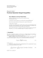
The sound detection and classification steps are repre-
sented in Figure 1. Only the colored blocks in the sound
recognition process will be addressed in this paper. For the
event detection task, the proposed approach which does not
require any pretrained models (unsupervised learning) is
based on the use of the exponential family model and 1-
SVMs to approximate the generalized likelihood ratio, thus
increasing robustness and allowing detecting events close to
each others. For the sound classification task, the proposed
approach presented has several original aspects, the most
prominent being the use of several 1-SVMs to perform mul-
tiple class classification and the use of a sophisticated dissim-
ilarity measure. In this paper, we will demonstrate that the 1-
SVM methodology creates reliable classifiers (i.e., classifiers
with very good generalization performance) more easy to
implement and tune than the common methods, while
having a reasonable computation cost.
The remainder of this paper is organized as follows.
Section 2 gives an overview of the 1-SVM-based learning
theory. We discuss the proposed 1-SVMs-based algorithms
andapproachestosounddetectioninSection 3 and to
sound classification in Section 4. Experimental results and
discussions are provided in Section 5. Section 6 concludes
the paper with a summary.
2. THE ONE-CLASS SVMs
The One-class approach [2] has been successfully applied

to various problems [10, 15, 25–27]. To denote a one-class
classification task, a large number of different terms have
been used in the literature. The term single-class classifica-
tion originates from Moya [28], but also outlier detection
[29], novelty detection [6, 23] or concept learning [30]
areused.Thedifferent terms originate from the different
applications to which one-class classification can be applied.
Obviously, its first application is outlier detection examples,
to detect uncharacteristic objects from a dataset, which do
not resemble the bulk of the dataset in some way. These out-
liers in the data can be caused by errors in the measurement
of feature values, resulting in an exceptionally large or small
feature value in comparison with other training objects. In
general, trained classifiers only provide reliable estimates for
input objects resembling the training set.
1-SVM distinguishes one class of data from the rest of
the feature space given only a positive data set (also known
as target data set) and never sees the outlier data. Instead, it
must estimate the boundary that separates those two classes
based only on data which lie on one side of it. The problem
therefore is to define this boundary in order to minimize
misclassifications by using a parameter to control the noise in
the training data and another one to control the smoothness
of the boundary.
The aim of 1-SVMs is to use the training dataset X
=
{
x
1
, , x

m
} in R
d
so as to learn a function f
X
: R
d
→ R
such that most of the data in X belong to the set R
X
={x ∈
R
d
with f
X
(x) ≥ 0}while the volume of R
X
is minimal. This
problem is termed minimum volume set (MVS) estimation
[31], and we see that membership of x to R
X
indicates
whether this datum is overall similar to X,ornot.Thus,by
learning regions R
X
i
for each class of sound (i = 1, , N),
we learn N membership functions f
X
i

. Given the f
X
i
’s, the
Asma Rabaoui et al. 3
Input audio
stream
Features
extraction
Event
detection
Events
boundaries
(a) Unsupervised events detection
Training
audio events
Features
extraction
Testing
audio events
Models
learning
Audio event recognized
(class assigned to event)
Calssifier
Supervised training of the audio events
Online testing (event classification)
(b) Supervised events classification
Figure 1: The event recognition process is composed into two main tasks: the sound detection task and the sound classification task. As
illustrated in (a), an unsupervised algorithm based on 1-SVMs will be applied to address the event detection task. In (b), a supervised

learning classification algorithm based on 1-SVMs will be proposed.
Separation hyperplane
W
Non-SVs
The smallest sphere
enclosing data (SVDD)
Hypersphere
S
Margin SV
Non-margin SV
(outlier)
O
Origin
ρ/
w
w

θ
ξ
i
/w
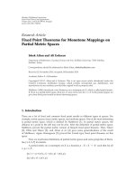
Figure 2: In the feature space H, the training data are mapped on a hypersphere S
(o,R=1)
. The 1-SVM algorithm defines a hyperplane with
equation W
={ ∈ H s.t. w, 
H
−ρ = 0}, orthogonal to w. Black dots represent the set of mapped data, that is, k(x
j
, ·), i = 1, ,m.For

RBF kernels, which depend only on x
− x

, k(x,x

) is constant, and the mapped data points thus lie on a hypersphere. In this case, finding
the smallest sphere enclosing the data is equivalent to maximizing the margin of separation from the origin.
assignment of a datum x to a class is performed as detailed in
Section 4.1.
1-SVMs solve MVS estimation in the following way. First,
aso-calledkernel function k(
·, ·); R
d
× R
d
→ R is selected,
and it is assumed to be positive definite [2]. Here, we assume
a Gaussian RBF kernel such that k(x, x

) = exp[−x −
x


2
/2σ
2
], where · denotes the Euclidean norm in R
d
. This
kernel induces a so-called feature space denoted by H via the

mapping φ :
R
d
→ H defined by φ(x)  k(x, ·), where H
is shown to be reproducing kernel Hilbert space (RKHS) of
functions, with dot product denoted by
·, ·
H
. (We stress on
the difference between the feature space, which is a (possibly
infinite dimensional) space of functions, and the space of
feature vectors,whichis
R
d
. Though confusion between these
two spaces is possible, we stick to these names as they
are widely used in the literature.) The reproducing kernel
property implies that
φ(x), φ(x

)
H
=k(x, ·), k(x

, ·)
H
=
k(x, x

) which makes the evaluation of k(x,x


) a linear
operation in H, whereas it is a nonlinear operation in
R
d
.In
the case of the Gaussian RBF kernel, we see that
φ(x)
2
H

φ(x), φ(x)
H
= k(x, x) = 1, thus all the mapped data
are located on the hypersphere with radius one, centered
onto the origin of H denoted by S
(o,R=1)
(Figure 2). The
1-SVM approach proceeds in feature space by determining
the hyperplane W that separates most of the data from the
hypersphere origin, while being as far as possible from it.
Since in H the image by φ of R
X
is included in the segment
of hypersphere bounded by W, this indeed implements MVS
estimation [31]. In practice, let W
={(·) ∈ H with
(·), w(·)
H
−ρ = 0}, then its parameters w(·)andρ result

from the optimization problem
min
w,ξ,ρ
1
2


w(·)


2
H
+
1
νm
m

j=1
ξ
j
−ρ (1)
4 EURASIP Journal on Advances in Signal Processing
subject to (for j = 1, , m)

w(·),k

x
j
, ·


H
≥ ρ −ξ
j
, ξ
j
≥ 0, (2)
where ν tunes the fraction of data that are allowed to be on
the wrong side of W (these are the outliers and they do not
belong to R
X
)andξ
j
’s are so-called slack variables. It can be
shown [2] that a solution of (1)-(2) is such that
w(
·) =
m

j=1
α
j
k

x
j
, ·

,(3)
where the α
j

’s verify the dual optimization problem
min
α
1
2
m

j,j

=1
α
j
α
j

k

x
j
, x
j


(4)
subject to
0
≤ α
j
≤
1

νm
,

j
α
j
= 1. (5)
Finally, the decision function is
f
X
(x) =
m

j=1
α
j
k

x
j
, x

−ρ (6)
and ρ is computed by using f
X
(x
j
) = 0 for those x
j
’s in X

that are located onto the boundary, that is, those that verify
both α
j
/
=0andα
j
/
=1/νm. An important remark is that the
solution is sparse, that is, most of the α
i
’s are zero (they
correspond to the x
j
’s which are inside the region R
X
,and
they verify f
X
(x) > 0).
As plotted in Figure 2, the MVS in H may also be
estimated by finding the minimum volume hypersphere that
encloses most of the data (support vector data description
(SVDD) [26, 32]), but this approach is equivalent to the
hyperplane one in the case of an RBF kernel.
In order to adjust the kernel for optimal results, the
parameter σ can be tuned to control the amount of smooth-
ing, that is, large values of σ lead to flat decision boundaries.
Also, ν is an upper bound on the fraction of outliers in the
dataset [2].
3. APPLICATION OF 1-SVMs TO SOUND DETECTION

The detection of an event (called the useful sound) is very
important because if an event is lost during the first step
of the system, it is lost forever. On the other hand, if there
are too many false alarms, the sound recognition system
is saturated. Therefore, the performance of the detection
algorithm is very important for the entire recognition
system. There are many techniques previously used for sound
detection with a very simple functional principle (a threshold
on energy), or with a statistical model [16, 33]. Very simple
methods based either on the variance or on the median
filtering of the signal energy have been used in many previous
works. In [34–36], three algorithms were used: one based
on the cross-correlation of two successive windows, a second
one based on the error of energy prediction, and a third one
based on the wavelet filtering. Another method widely used
in the speech community is based on model selection using
Bayesian information criterion (BIC) [20]. Our objective
is to develop a new robust unsupervised sound detection
technique based on a new 1-SVMs-based algorithm that uses
the exponential family model. In this section, we begin by
giving a brief description of some previous works with a
special emphasis on the BIC detection method.
3.1. Previous works
Sound detection is the first step of every sound analysis
system and is necessary to extract the significant sounds
before initiating the classification step. Here, we present
four classical event detection algorithms: cross-correlation,
energy prediction, wavelet filtering, and BIC. The first three
methods are widely used for impulsive sound detection [34]
and they are based on the energy calculation and use a

threshold which must be settled empirically. In recent years,
the last method, BIC, has attracted more attention in the
speech community and has been applied in many statistical
sound detection methods especially for speaker change
detection [17–20]. The Bayesian information criterion is a
model selection criterion that was first proposed by [37]and
widely used in the statistical literature.
The cross-correlation detection method is based on
the measure of similarity between two successive signal
windows in order to find abrupt changes of the signal. The
algorithm calculates the cross-correlation function between
two windows and keeps the maximum value. Finally, a
threshold on this signal is applied (if the signal is under
the threshold, an event detection is generated) [34]. The
energy prediction-based detection method computes the
signal energy on N sample windows. The next value of
the energy is predicted based on the L previous values (L
= prediction length) using the spline interpolation method
[36]. Finally, a threshold is settled on the prediction error
(the absolute difference between the real value and the
predicted value). The wavelet filtering-based sound detection
method [35]useswaveletssuchasDaubechiestocompute
DWT [38]. The sound detection algorithm computes the
energy of the high-order wavelet coefficients which are the
most significant coefficients for short and impulsive signals.
The sound detection is achieved by applying a threshold on
the sum of energies.
The change detection via BIC algorithm [20]isbasedon
the measure of the ΔBIC [39]valuebetweentwoadjacent
windows. The sequence containing these two windows is

modeled as one or two multivariate Gaussian distributions.
The null hypothesis that the entire sequence is drawn from a
single distribution is compared to the hypothesis that there
is a segment boundary between the two windows which
means that the two windows are modeled by two different
distributions. When the BIC difference between the two
models is positive (ΔBIC > 0), we place a segment boundary
between the two windows, and then begin searching again to
the right of this boundary [18].
Asma Rabaoui et al. 5
3.2. Sound detection using 1-class SVM
and exponential family
In most commonly used model selection sound detection
techniques such as the BIC detection method previously
described, the basic problem may be viewed as a two-class
classification. Where the objective is to determine whether N
consecutive audio frames constitute a single homogeneous
window W or two different windows W
1
and W
2
.In
order to detect if an abrupt change occurred at the ith
frame within a window of N frames, two models are built.
One which represents the entire window by a Gaussian
characterized by μ (mean), Σ (variance); a second which
represents the window up to the ith frame, W
1
with μ
1

,
Σ
1
and the remaining part, W
2
, with a second Gaussian
μ
2
, Σ
2
. This representation using a Gaussian process is not
totally exact when abrupt changes are close to each other
especially when the events to be detected are too short and
impulsive. To solve this problem, our proposed technique
uses 1-SVMs and exponential family model to maximize the
generalized likelihood ratio with any probability distribution
of windows.
3.2.1. Exponential family
The exponential family covers a large number (and well-
known classes) of distributions such as Gaussian, multino-
mial, and poisson. A general representation of an exponential
family is given by the following probability density function:
p(x
| η) = h(x)exp

η
T
T(x) −A(η)

,(7)

where h(x) is called the base density which is always
≥ 0, η is
the natural parameter, T(x) is the sufficient statistic vector,
and A(η) is the cumulant generating function or the log
normalizer.
ThechoiceofT(x)andh(x) determines the member
of the exponential family. Also we know that since this is a
density function,

h(x)exp

η
T
T(x) −A(η)

dx = 1, (8)
then
A(η)
= log

exp

η
T
T(x)

h(x)dx. (9)
For a Gaussian distribution, p(x
| μ,σ
2

) = (1/
√
2π)
exp((μ/σ
2
)x − (1/2σ
2
)x
2
− (μ
2
/2σ
2
) − log σ). In this case,
h(x)
= 1/
√
2π, η = [μ/σ
2
, −1/2σ
2
], and T(x) = [x, x
2
]. Thus,
Gaussian distribution is included in the exponential family.
The density function of an exponential family can be
written in the case of presence of a reproducing kernel
Hilbert space H with a reproducing kernel k as
p(x
| η) = h(x)exp


η(·), k(x, ·)

H
−A(η)

(10)
with
A(η)
= log

exp

η(·), k(x, ·)

H

h(x)dx. (11)
3.2.2. Applying 1-SVM to sound detection
Novelty change detection theory using SVM and exponential
family was first proposed in [40, 41]. In this paper, this prob-
lem will be addressed with novel sophisticated approaches.
Let X
={x
1
, x
2
, , x
N
} and Y ={y

1
, y
2
, , y
N
} be two
adjacent windows of acoustic feature vectors extracted from
the audio signal, where N is the number of data points in one
window. Let Z denote the union of the contents of the two
windows having 2N data points. The sequences of random
variables X and Y are distributed according to
Px and Py
distribution, respectively. We want to test if there exists a
sound change after the sample x
N
between the two windows.
The problem can be viewed as testing the hypothesis H
0
:
P
x
= P
y
against the alternative H
1
: Px
/
=Py. H
0
is the null

hypothesis and represents that the entire sequence is drawn
from a single distribution, thus there exists only one sound.
While H
1
represents the hypothesis that there is a segment
boundary after sample X
n
, the likelihood ratio test of this
hypotheses test is the following:
L

z
1
, , z
2N

=

N
i
=1
P
x

z
i


2N
i

=N+1
P
y

z
i


2N
i
=1
P
x

z
i

=
2N

i=N+1
P
y

z
i

P
x


z
i

.
(12)
Since both densities are unknown, the generalized likelihood
ratio (GLR) has to be used:
L

z
1
, , z
2N

=
2N

i=N+1

P
y

z
i


P
x

z

i

, (13)
where

P
0
and

P
0
are the maximum likelihood estimates of
the densities.
Assuming that both densities
P
x
and P
y
are included
in the generalized exponential family, thus there exists a
reproducing kernel Hilbert space H embedded with the dot
product
·, ·
H
with a reproducing kernel k such that in (10):
P
x
(z) = h(z)exp

η

x
(·), k(z, ·)

H
−A

η
x

,
P
y
(z) = h(z)exp

η
y
(·), k(z, ·)

H
−A

η
y

.
(14)
Using 1-SVM and the exponential family, a robust
approximation of the maximum likelihood estimates of the
densities
P

x
and P
y
can be written as

P
x
(z) = h(z)exp

N

i=1
α
(x)
i
k

z, z
i

−
A

η
x


,

P

y
(z) = h(z)exp

2N

i=N+1
α
(y)
i
k

z, z
i

−
A

η
y


,
(15)
where α
(x)
i
is determined by solving the one 1-SVM problem
on the first half of the data (z
1
to z

N
), while α
(y)
i
is given by
solving the 1-SVM problem on the second half of the data
6 EURASIP Journal on Advances in Signal Processing
(z
N+1
to z
2N
). Using these three hypotheses, the generalized
likelihood ratio test is approximated as follows:
L

z
1
, , z
2N

=
2N

j=N+1
exp


2N
i
=N+1

α
(y)
i
k

z
j
, z
i

−
A

η
y


exp


2N
i
=1
α
(x)
i
k

x
j

, x
i

−A

η
x


.
(16)
A sound change in the frame z
n
exists if
L

z
1
, , z
2N

>s
x
⇐⇒
2N

j=N+1

2N


i=N+1
α
(y)
i
k

z
j
, z
i

−
N

i=1
α
(x)
i
k

z
j
, z
i


>s

x
,

(17)
where s
x
is a fixed threshold. Moreover,

2N
i
=N+1
α
(y)
i
k(z
j
, z
i
)
is very small and can be neglected in comparison with

N
i
=1
α
(x)
i
k(z
j
, z
i
). Then a sound change is detected when
2N


j=N+1

−
N

i=1
α
(x)
i
k

z
j
, z
i


>s

x
. (18)
3.2.3. Sound detection criterion
Previously, we showed that a sound change exists if the
condition defined by (18) is verified. This sound detection
approach can be interpreted like this: to decide if a sound
change exits between the two windows X and Y,webuiltan
SVM using the data X as learning data, then Y data are used
for testing if the two windows are homogenous or not.
On the other hand, since H

0
represents the hypothesis
of
P
x
= P
y
, the likelihood ratio test of the hypotheses test
described previously can be written as
L

z
1
, , z
2N

=

N
i=1
P
x

z
i


2N
i=N+1
P

y

z
i


2N
i
=1
P
y

z
i

=
N

i=1
P
x

z
i

P
y

z
i


.
(19)
Using the same gait, a sound change has occurred if
N

j=1

−
2N

i=N+1
α
(y)
i
k

z
j
, z
i


>s

y
. (20)
Preliminary empirical tests show that in some cases it is
more appropriate to apply two training rounds: after using
X data for learning and Y data for testing, we can use Y

data for learning and X data for testing. This procedure
provides more detection accuracy. For that reason, it is more
appropriate to use the criterion described as follow:
2N

j=N+1

−
N

i=1
α
(x)
i
k

z
j
, z
i


+
N

j=1

−
2N


i=N+1
α
(y)
i
k

z
j
, z
i


>S,
(21)
where S
= s

x
+ s

y
.Equation(21) can be considered as
a distance measure between two datasets. Obviously, higher
values of this distance indicate that the two dataset distribu-
tions are not similar.
Audio stream
Audio
parameterization
Train data
SVM 1

Te s t d a t a
SVM 2
Train data
SVM 2
Te s t d a t a
SVM 1
Distance measure
d
1
Distance measure
d
2
Detection criterion: d = d
1
+ d
2
Distance curve
 Significant  peaks detection
Break points detection
= sound detection
New limits of
the analysis frame
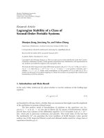
Figure 3: Block diagram of our sounds detection approach. The
method is based on a new distance measure d between two adjacent
analysis windows. This distance is the sum of d
1
in (18)andd
2
in
(20). d

1
is obtained by using training dataset from the first window
and testing dataset from the second one. d
2
is computed by inverting
the datasets.
3.2.4. Our sound detec tion method
Our technique of sound detection is based on the computa-
tion of the distance detailed in (21)betweenapairofadjacent
windows of the same size shifted by a fixed step along the
whole parameterized signal. This allows to obtain the curve
of the variation of the distance in time. The analysis of this
curve shows that a sound change point is characterized by
the presence of a “significant” peak. A peak is regarded as
“significant” when it presents a high value. So, break points
can be detected easily by searching the local maxima of
the distance curve that presents a value higher than a fixed
threshold (Figure 3).
4. APPLICATION OF 1-SVMs TO
SOUNDS CLASSIFICATION
In audio classification systems, the most popular approach
is based on hidden Markov models (HMMs) with Gaussian
mixture observation densities. These systems typically use
a representational model based on maximum likelihood
decoding and expectation maximization-based training. Th-
ough powerful, this paradigm is prone to overfitting and does
Asma Rabaoui et al. 7
not directly incorporate discriminative information. It is
shown that HMM-based sound recognition systems perform
very well on closed-loop tests but performance degrades

significantly on open-loop tests. In [42], we showed that
this is specially true for impulsive sound classification. As
an attempt to overcome these drawbacks, artificial neural
networks (ANNs) have been proposed as a replacement for
the Gaussian emission probabilities under the belief that
the ANN models provide better discrimination capabilities.
However, the use of ANNs often results in overparameterized
models which are also prone to overfitting.
This can be attributed to the fact that most systems do
not generalize well. We need systems with good general-
ization properties where the worst case performance on a
given test set can be bounded as part of the training process
without having to actually test the system. With many real-
world applications where open-loop testing is required, the
significance of generalization is further amplified.
The application addressed here concerns real-world
sound classification. In real environment, there might be
many sounds which do not belong to one of the predefined
classes, thus it is necessary to define a rejection class,which
may gather all sounds which do not belong to the training
classes. An easy and elegant way to do so consists of esti-
mating the regions of high probability of the known classes
in the space of features, and considering the rest of the
space as the rejection class. Training several 1-SVMs does this
automatically.
In order to enhance the discrimination ability of the
proposed classification method, the discrimination rule illus-
trated by (6) will be replaced by a sophisticated dissimilarity
measure described in the subsection below.
4.1. A dissimilarity measure

The 1-SVM can be used to learn the MVS of a dataset of
feature vectors which relate to sounds. In the following, we
will define a dissimilarity measure by adapting the results
of [13, 15]. Assume that N 1-SVMs have been learnt from
the datasets
{X
1
, , X
N
}, and consider one of them, with
associated set of coefficients denoted (
{α
j
}
j=1, ,m
, ρ). In
order to determine whether a new datum x is similar to the
set X, we will define a dissimilarity measure, denoted by
d(X,x), and deduced from the decision function f
X
(x) =

m
j=1
α
j
k(x
j
, x) −ρ,inwhichρ is seen as a scaling parameter
which balances the α

j
’s. Thanks to this normalization, the
comparison of such dissimilarity measures d(X
i
, x)and
d(X
i

, x) is possible. Indeed,
d(X,x)
=−log


w(·),k(x, ·)

H
ρ

=−
log



w(·)


H
ρ
cos


w(·)∠k(x, ·)


,
(22)
because
k(x, ·)
H
= 1, where w(·)∠k(x, ·) denotes the
angle between w(
·)andk(x, ·).
By doing elementary geometry in feature space, we can
show that ρ/
w(·)
H
= cos(

θ)(Figure 2). This yields the
following interpretation of d(X, x):
d(X,x)
=−log

cos

w(·)∠k(x, ·)

cos


θ



. (23)
Finally, the following relation
log

m

j=1
α
j
k

x, x
j


+log[ρ]
= log

w(·),k(x, ·)

H

+log[ρ] = d(X,x)
(24)
shows that the normalization is sound, and makes d(X, x)a
valid tool to examine the membership of x to a given class
represented by a training set X.
4.2. Multiple sound classes in 1-SVM-based

classification algorithm
The sound classification algorithm comprises three main
steps. Step one is that of training data preparation, and it
includes the selection of a set of features which are computed
for all the training data. The value of ν is selected in the
reduced interval [0.05, 0.8] in order to avoid edge effects for
small or large values of ν.
We adopt the following notations. We assume that X
=
{
x
1
, , x
m
}is a dataset in R
d
. Here, each x
j
is the full feature
vector of a signal, that is, each signal is represented by one
vector x
j
in R
d
.LetX be the set of training sounds, shared
in N
c
classes denoted by X
1
, , X

N
c
. Each class contains m
i
sounds, i = 1, , N
c
.
Algorithm 1 (Sound classification algorithm).
Step 1 (Data preparation). (i) Select a set of features.
(ii) Form the training sets X
i
={x
i,1
, , x
i,m
i
}, i = 1, ,
N
c
by computing these features and forming the feature
vectors for all the training sounds selected.
(iii) Set the parameter σ of the Gaussian RBF kernel to
some pre-determined value (e.g., set σ as half the average
euclidean distance between any two points x
i,j
and x
i

,j


[3]),
and select ν
∈ [0.05, 0.8].
Step 2 (Training step). (i) For i
= 1, , N
c
, solve the 1-SVM
problem for the set X
i
, resulting in a set of coefficients (α
i,j
,
ρ
j
), j = 1, , m
i
.
Step 3 (Testing step). (i) For each sound s to be classified into
one of the N
c
classes, do
(1) compute its feature vector, denoted x,
(2) for i
= 1, , N
c
,computed(X
i
, x) by using (24),
(3) assign the sound s to the class


i such that

i = arg
min
i=1, ,N
c
d(X
i
, x).
8 EURASIP Journal on Advances in Signal Processing
Table 1: Classes of sounds and number of samples in the database
used for performance evaluation.
Classes Total number Total duration (s)
Human screams (C1) 73 189
Gunshots (C2) 225 352
Glass breaks (C3) 88 143
Explosions (C4) 62 180
Door slams (C5) 314 386
Dog barks (C6) 55 97
Phone rings (C7) 51 107
Children voices (C8) 87 140
Machines (C9) 60 184
Total 1015 1778
5. EXPERIMENTS ON SOUND DETECTION
AND CLASSIFICATION
5.1. Experimental setup
The major part of the sound samples used in the sound
recognition experiments is taken from different sound
libraries available on the market [43, 44]. Considering several
sound libraries is necessary for building a representative,

large, and sufficiently diversified database. Some particular
classes of sounds have been built or completed with hand-
recorded signals. All signals in the database have a 16-bit
resolution and are sampled at 44100 Hz.
During database construction, great care was devoted
to the selection of the signals. When a rather general use
of the sound recognition system is required, some kind of
intraclass diversity in the signal properties should be inte-
grated in the database. Even if it would be better for a given
sound recognition system, to be designed for the specific
type of encountered signals, it was decided in this study to
incorporate sufficiently diverse signals in the same category.
As a result, one class of signals can be composed by
very different temporal or spectral characteristics, amplitude
levels, and duration and time location.
The selected sounds are impulsive and they are typical
of surveillance applications. The number and duration of
considered samples for each sound category is indicated in
Ta ble 1 .
Furthermore, other nonimpulsive classes of sounds (ma-
chines, children voices) are also integrated in the experimen-
tation. We note that the number of items in each class is
deliberately not equal, and sometimes very different. More-
over, explosion and gunshot sounds are very close to each
other. Even for a person, it is sometimes not obvious to
discriminate between them. They are intentionally differen-
tiated to test ability of the system in separating very close
classes of sounds.
5.2. Sound detection experiments
This section presents sound detection results with exper-

iments conducted on an audio stream with length more
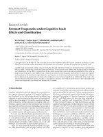
Target break
point sequence
Detected break
point sequence
Real break points
Missed detection
To l e r a n c e
Tr ue d e te ct ed
break points
False alarm
Figure 4: Example of a missed detection and a false alarm of a
change point.
than 30 minutes containing the sounds (events) described
in Ta bl e 1 . After extracting the feature vectors (using a
frame with length 25 ms and 50% overlap), a sliding analysis
window of a fixed length was used. This value is the result of
atradeoff between the number of frames inside the analysis
windows required for significant statistical estimation and
for the fact that this analysis window must not contain more
than one sound change point. The sounds to be detected are
short and impulsive, thus the window analysis length was
fixed to 1.4 seconds.
A change sound detection system has two possible types
of error. Type-I-errors occur if a true change is not spotted
within a certain window (missed detection). Type-II-errors
occur when a detected change does not correspond to a true
change in the reference (false alarm). Figure 4 illustrates an
example of the missed detection, false alarm and change-
point tolerance evaluation for the audio detection task. In the

conducted experiments, we considered that a change point is
detected using a certain tolerance settled to 0.4 second.
Type-I and -II errors are also referred to as precision
(PRC) and recall (RCL), respectively, wich are defined as
PRC
=
Number of correctly found changes
Total number of changes found
,
RCL
=
Number of correctly found changes
Total number of correct changes
.
(25)
In order to compare the performance of different sys-
tems, the F-measure is often used and is defined as
F
=
2.0 ×PRC ×RCL
PRC + RCL
. (26)
The F-measure varies from 0 to 1, with a higher F-
measure indicating better performance.
The results using the proposed technique (1-SVM)
and the other classical approaches (cross-correlation (CC),
energy prediction (EP), wavelet filtering (WF), and BIC) are
presented below. All the studied techniques use a threshold
that must be fixed empirically and the experimental curves
Asma Rabaoui et al. 9

0.850.80.750.70.650.60.55
PRC
WF
BIC
CC
EP
1-SVM
0.5
0.55
0.6
0.65
0.7
0.75
0.8
0.85
0.9
RCL
Figure 5: RCL versus PRC curves of the proposed 1-SVMs-based
sound detection methods against the other classical approaches.
were obtained by varying this threshold. In theory, the
BIC-based method did not use any threshold. However, in
previous works [20], it has been shown that the ΔBIC uses
a parameter λ that must be settled empirically and this
parameter was considered as a hidden threshold.
Figure 5 presents a recall (RCL) versus a precision (PRC)
plot for the different studied methods. We can notice that
the proposed 1-SVM-based sound detection method outper-
forms the others. Figures 6 and 7 illustrate the performance
of the detection with different MFCC orders. This study
experimented on three different MFCC orders: 13, 26, and

39. Generally, the 13 MFCCs include 12 MFCCs and onelog
energy. The 26 MFCCs include the 13 MFCCs and their first-
time derivatives, and the 39 MFCCs include the 13 MFCCs
and theirs first- and second-time derivatives. As presented
in Figure 6, the features with higher dimensions give fewer
errors in parameter estimation and better detection perfor-
mance. This is due to the fact that 1-SVMs are not sensitive
to the dimensionality of the feature vectors. However, using
26 MFCCs and 39 MFCCs with BIC gives low values of PRC
and RCL compared to those obtained using 13 MFCCs.
The best results achieved using all the studied methods
are illustrated in Ta ble 2 . The PRC and RCL values obtained
with the sound detection method based on BIC are lower
than the proposed method (PRC
= 0.72, RCL = 0.73). This
is due essentially to the presence of short sounds that can be
close to each others. In this case, we do not have enough data
for the good estimation of the BIC parameters. To avoid this
deficiency, we used 1-SVMs with the exponential family.
Results obtained with cross-correlation, energy predic-
tion, and wavelet filtering methods show that using only an
energy-based criterion to detect events is not very appropri-
ate when there are sounds that present similar characteristics
and which are very close to each others. With wavelet fil-
tering, a slightly better result was obtained because it leads
to better characterize the acoustical properties of complex
audio scenes.
Sound detection using the proposed method based on 1-
SVMs presents better results than all the other techniques. In
0.90.850.80.750.7

PRC
Number of MFCCs
= 13
Number of MFCCs
= 26
Number of MFCCs
= 39
0.65
0.7
0.75
0.8
0.85
0.9
RCL
Figure 6: RCL versus PRC curves of the effect of the MFCC order
in the proposed 1-SVMs-based method.
0.80.780.760.740.720.70.680.660.640.62
PRC
Number of MFCCs
= 13
Number of MFCCs
= 26
Number of MFCCs
= 39
0.62
0.64
0.66
0.68
0.7
0.72

0.74
0.76
0.78
0.8
RCL
Figure 7: RCL versus PRC curves of the effect of the MFCC order
in the BIC-based method.
Table 2: Sound detection results using various techniques.
Techniques RCL PRC F
1-SVM 0.85 0.86 0.85
Wavelet filtering 0.77 0.76 0.76
BIC 0.73 0.72 0.72
Cross-correlation 0.68 0.70 0.69
Energy prediction 0.61 0.63 0.62
fact, the obtained higher value of PRC (0.86) indicates that
our technique avoids many false alarms. Moreover, by using
this method, we can detect approximately the major break
points that exist in the audio stream (higher RCL
= 0.85).
5.3. Sound classification experiments
In this section, we will present classification results obtained
by applying Algorithm 1. Features are computed from all the
10 EURASIP Journal on Advances in Signal Processing
Table 3: Confusion Matrix obtained by using a feature vector containing 12 cepstral coefficients MFCC + Energy + Logenergy + SC + SRF.
1-SVMs are applied with an RBF kernel (σ
= 10).
C1 C2 C3 C4 C5 C6 C7 C8 C9
C110000000000
C2 0 90.66 0 9.33 0 0 0 0 0
C3 0 0 93.33 0 6.66 0 0 0 0

C4 0 20.05 0 75.19 4.76 0 0 0 0
C5 0 0.95 0 1.9 97.14 0 0 0 0
C6 0 0 0 0 5.26 94.73 0 0 0
C700000010000
C8 0 0 0 3.45 3.45 0 0 93.1 0
C900000000100
Total recognition rate = 93.79%
Table 4: Confusion Matrix obtained by using a feature vector containing 12 cepstral coefficients MFCC + Energy + Logenergy + SC + SRF.
M-SVMs(1-vs-1) are applied with an RBF kernel (σ
= 10).
C1 C2 C3 C4 C5 C6 C7 C8 C9
C110000000000
C2 0 88.15 2.19 9.66 0 0 0 0 0
C3 0 0 90.33 0 6.66 0 3 0 0
C4 0 20.05 0 75.19 4.76 0 0 0 0
C5 0 0.95 0 3.9 95.14 0 0 0 0
C6 0 0 0 0 5.26 94.73 0 0 0
C7 0 0 1.2 9.66 0 0 89.14 0 0
C8 0 0 0 13.45 3.45 0 0 83.1 0
C900000000100
Total recognition rate = 90.64%
samples in each sound (segment). The analysis window is
Hamming with length 25 milliseconds and 50% overlap. The
selected feature vector contains 12 Mel-frequency cepstral
coefficients (MFCCs), the energy, the Logenergy, the Spectral
Centrod (SC), and the spectral rolloff point (SRF). More
details about these features and theirs computations can be
found in our previous work [24, 45]. The used database is
illustrated in Ta bl e 1, 70% of the samples are used for the
training set and 30% for the testing set.

Evaluations on the 1-SVM-based system using a Gaus-
sian RBF kernel with individual features are compared to the
results obtained by the M-SVM-based classifiers (multiclass)
and by a baseline HMM-based classifier.
A multiclass pattern sound recognition system can be
obtained from two-class SVMs. The basis theory of SVM for
two-class classification in beyond the scope of this paper (see
our previous works for more details [46]). There are gener-
ally two schemes for this purpose. One is the one-versus-all
(1-vs-all) strategy to classify between each class and all the
remaining; the other is the one-versus-one (1-vs-1) strategy
to classify between each pair. However, the best method of
extending the two-class classifier to multiclass problems is
not clear. The 1-vs-all approach works by constructing for
each class a classifier which separates that class from the
remainder of the data. A given test example is then classified
as belonging to the class whose boundary maximizes the
margin. The 1-vs-1 approach simply constructs for each pair
of classes a classifier which separates those classes. A test
example is then classified by all of the classifiers, and is said
to belong to the class with the largest number of positive
outputs from these subclassifiers.
Moreover, for a complete comparison task between
classifiers, we choose to train a statistical model for each
audio class using multi-Gaussian hidden Markov models
(HMMs). More details about HMMs can be found in
our previous work [42], where we reported an advanced
application of adapted HMMs for sounds classification.
During training, by analyzing the feature vectors of the
training set, the parameters for each state of an audio model

are estimated using the well-known Baum-Welch algorithm
[22]. The procedure starts with random initial values for all
of the parameters and optimizes the parameters by iterative
reestimation. Each iteration runs through the entire set of
training data in a process that is repeated until the model
converges to satisfactory values [21, 47]. A specific HMM
topology is used to describe how the states are connected.
The temporal structures of audio sequences for an isolated
sound recognition problem require the use of a simple
Asma Rabaoui et al. 11
Table 5: Confusion Matrix obtained by using a feature vector containing 12 cepstral coefficients MFCC + Energy + Logenergy + SC + SRF.
M-SVMs(1-vs-all) are applied with an RBF kernel (σ
= 10).
C1 C2 C3 C4 C5 C6 C7 C8 C9
C110000000000
C2 0 88.76 2.24 6.33 0 2.66 0 0 0
C3 0 0 94.23 0 2.76 0 3 0 0
C4 0 20.09 0 75.15 4.76 0 0 0 0
C5 0 0.95 0 3.9 95.14 0 0 0 0
C6 0 0 0 0 5.26 94.73 0 0 0
C7 0 0 1.2 9.66 0 0 89.14 0 0
C8 0 0 0 13.45 12.62 0 0 73.93 0
C900000000100
Total recognition rate = 90.12%
left-right topology with five states in total. Three of these
are emitting states and have output probability distributions
associated with them. Our system uses continuous density
models in which each observation probability distribution
is represented by a mixture Gaussian density. The optimum
number of mixture components N

G
in each state is reached
by applying a mixture incrementing.
Ta ble s 3–6 present some confusion matrices illustrating
the best results for the different tested classifiers. The
performance rate is computed as the percentage number of
sounds correctly recognized and it is given by (H/N)
×100%,
where H is the number of correct sounds and N is the total
number of sounds to be recognized.
In order to provide a comparison point, we conducted
experiments using HMMs, M-SVM(1-vs-1), and M-SVM(1-
vs-all). By comparison with the other studied classifiers, the
use of 1-SVMs is plainly justified by the results presented
here, as it yields consistently lower-error rate and a high-
classification accuracy.
Due to the need to estimate several classifiers, if we used
1-vs-1 or 1-vs-all approaches to solve an N-class classifi-
cation problem in computationally restricted environments
this can be a serious impediment. In conclusion, though
SVMs are well-founded mathematically to achieve good gen-
eralization while maintaining a high-classification accuracy,
we need to consider issues such as computation complexity
and ease of implementation in order to choose the best
classifier approach for a given application.
1-vs-1 classifiers learn to discriminate one class from
another class and 1-vs-all classifiers learn to discriminate
one class from all other classes. 1-vs-1 classifiers are typically
smaller and can be estimated using fewer resources than 1-
vs-all classifiers. When the number of classes is N we need

to estimate N(N
− 1)/2 1-vs-1 classifiers as compared to 1-
vs-all classifiers. On several standard classification tasks, it
has been proven that 1-vs-1 classifiers are marginally more
accurate than 1-vs-all classifiers. In most cases, the number
of 1-vs-1 classifiers that need to be estimated is significantly
greater that 1-vs-all classifiers and estimating these classifiers
can be very time consuming. In fact, using 1-vs-1 classifiers
makes each individual training problem smaller, and hence
55504540353025201510510.50.1
σ
0
10
20
30
40
50
60
70
80
90
Correct classification (%)
Figure 8: Influence of the parameter σ in a Gaussian RBF kernel
on the accuracy of the proposed 1-SVM-based classification task,
when using validation sets and an iteration number P,asdetailedin
Algorithm 1.
the memory CPU time required to train each classifier is
greatly reduced, but the number of classifiers to be trained
is high. While using a 1-vs-all approach requires many fewer
classifiers to be trained, the memory requirements to train

each classifier were found to be prohibitive. We used both 1-
vs-1 and 1-vs-all classifiers in our experiments reported here
in order to apply a complete comparison with the proposed
1-SVM classifier.
Overall, we found the 1-SVM methodology more easy to
implement and tune and well adapted to large dimensional
feature vectors, while having a reasonable training cost.
The SVM model has two parameters that have to be
adjusted: ν and σ. We first addressed the problem of tuning
the kernel parameter σ. There are several possible criterions
for selecting σ such as minimizing the number of support
vectors, maximizing the margin of separation from the
origin, and minimizing the radius of the smallest sphere
enclosing the data [48]. Figure 8 shows a plot of the second
criterion as a function of σ. As can be seen, using validation
sets to do cross-validation is of course a good way to tune
12 EURASIP Journal on Advances in Signal Processing
Table 6: Confusion Matrix obtained with HMMs (N
G
= 3 and 5 iterations in the Baum-Welch algorithm are applied) using a feature vector
containing 12 cepstral coefficients MFCC + Energy + Logenergy + SC + SRF.
C1 C2 C3 C4 C5 C6 C7 C8 C9
C197.6600002.33000
C2 0 90.66 0 9.33 0 0 0 0 0
C3 0 0 96.33 0 3.66 0 0 0 0
C4 0 9.05 0 86.19 4.76 0 0 0 0
C5 0 0.95 0 1.9 97.14 0 0 0 0
C600005.2694.73000
C7 0 0 4.76 2.05 7 0 86.19 0 0
C8 0 0 0 3.45 3.45 0 0 93.1 0

C9 0 0 7.66 0 2.85 3.16 1.33 0 85.01
Total recognition rate = 91.89%
Table 7: Sound recognition rates for various values of ν applied to
1-SVMs- and M-SVMs-based classifiers.
ν 1-SVM M-SVM(1-vs-1) M-SVM(1-vs-all)
0.1 92.33 90.64 90.12
0.293.79 90.64 90.12
0.3 92.33 90.64 90.12
0.4 92.33 89.50 88.73
0.5 91.33 88.50 87.73
0.6 91.93 89.66 88.46
0.7 85.46 82.12 81.73
0.8 80.50 75.23 72.33
the kernel parameter, σ. From the dataset, we were able to
make validation sets and use them to examine the classi-
fication accuracy of the classifier as a function of σ.For
asufficiently large training set, it is possible to select the
optimal parameters by applying an original cross-validation
procedure [49].
σ must be tuned to control the amount of smoothing
because the good performance of RBF kernels highly relies on
the choice of this parameter. Figure 8 shows the performance
of 1-SVMs using an RBF kernel versus σ. It is interesting to
point out the behavior of a 1-SVM with an RBF kernel when
σ becomes too small and when it becomes too large. When
σ becomes too small, all the training examples are support
vectors. This means that the 1-SVM learns by heart and then
is unable to generalize. But, when σ becomes too large, the
RBF kernel will be equivalent to the linear kernel and this
leads to flat decision boundaries.

We conducted also some experiences in Table 7 to show
the effect of the parameter ν. The 1-SVM algorithm performs
well with the small values of ν. Since the smaller values of ν
correspond to the smaller number of outliers, this leads to
the larger region capturing most of the training points. It was
decided (Ta b le 7 ) to only allow 20% classification error on
the training data, that is, ν
= 0.2.
We can remark that splitting the multiclass problem
into several two classes subproblems is an approach which
is generally quite precise when the number of classes is
small (typically up to 5), and when the number of training
data is reasonable. Indeed, all the data of all classes are used
to train the multiclass SVM, which scales typically from
O((

N
c
i=1

N
c
i

=1, ,N
)
i

/
=i

(m
i
+ m
i

)
3
)toO((

N
c
i=1
m
i
)
3
)(each
class i contains m
i
sounds). However, the 1-SVM approach
can be generalized to any number of classes, and the com-
putational cost for training scales with O(

N
c
i=1
m
3
i
), which

may be far quicker than any of the multiple class approaches.
In conclusion, due to the need to estimate several classi-
fiers if using 1-vs-1 or 1-vs-all approaches to solve an N-class
classification problem, in computationally restricted envi-
ronments, this can be a serious impediment. Thus, though
SVMs are well founded mathematically to achieve good
generalization while maintaining a high-classification accu-
racy, we need to consider issues such as computation
complexity and ease of implementation in order to choose
the best classifier approach for a given application. Hence,
in situations where accuracy and generalization are the only
most important criterions for selection, we can confirm
that both M-SVM strategies should be explored. In the
literature, 1-vs-1 classifiers had been shown to perform
better than 1-vs-all classifiers in many classification tasks.
This conclusion is also confirmed in Ta bl e 7 .Thereare,
however, other practical issues for this choice, using 1-vs-
1 classifiers makes the problem of each individual training
smaller, and hence the memory CPU time required to train
each classifier is greatly reduced. While using a 1-vs-all
approach requires many fewer classifiers to be trained, the
memory requirements to train each classifier were found to
be prohibitive.
6. CONCLUSION
In this paper, we have proposed a new unsupervised sound
detection algorithm based on 1-SVMs. This algorithm out-
performs classical sound detection methods. Using the
exponential family model, we obtain a good estimation of the
generalized likelihood ratio applied on the known hypothesis
test generally used in change-detection tasks. Experimental

results present higher precision and recall values than those
obtained with classical sound detection techniques.
Asma Rabaoui et al. 13
Moreover, we have developed a multiclass classification
strategy by using 1-SVMs to solve a sound classification
problem. The proposed system uses a discriminative method
based on a sophisticated dissimilarity measure, in order to
classify a set of sounds into predefined classes.
There is still room for improvement in the proposed
approaches. In particular, our future research will be focused
on addressing the following issues. First, in order to process
in real time, the available data to train models either for
sound detection or classification are always limited. Estimat-
ing an accurate model from limited training data is still a
challenge. Also, in real-world conditions, the complexity of
the application context affects negatively segmentation and
classification results.
REFERENCES
[1] V. Vapnik, Statistical Learning Theory, John Wiley & Sons, New
York, NY, USA, 1998.
[2] B. Sch
¨
olkopf and A. Smola, Learning with Kernels, MIT Press,
Cambridge, Mass, USA, 2002.
[3] N. Smith and M. Gales, “Speech recognition using SVMs,” in
Advances in Neural Information Processing Systems 14,T.G.
Dietterich, S. Becker, and Z. Ghahramani, Eds., pp. 1197–
1204, MIT Press, Vancouver, Canada, December 2001.
[4] V. Wan and S. Renals, “Evaluation of kernel methods for spe-
aker verification and identification,” in Proceedings of IEEE

International Conference on Acoustics, Speech and Signal Pro-
cessing (ICASSP ’02), vol. 1, pp. 669–672, Orlando, Fla, USA,
May 2002.
[5] C. J. C. Burges, J. C. Platt, and S. Jana, “Extracting noise-
robust features from audio data,” in Proceedings of IEEE Inter-
national Conference on Acoustics, Speech and Signal Processing
(ICASSP ’02), vol. 1, pp. 1021–1024, Orlando, Fla, USA, May
2002.
[6] M. Davy and S. Godsill, “Detection of abrupt spectral changes
using support vector machines: an application to audio signal
segmentation,” in Proceedings of IEEE International Conference
on Acoustics, Speech and Signal Processing (ICASSP ’02), vol. 2,
pp. 1313–1316, Orlando, Fla, USA, May 2002.
[7] E. Osuna, R. Freund, and F. Girosi, “Training support vector
machines: an application to face detection,” in Proceedings of
the IEEE Computer Society Conference on Computer Vision and
Pattern Recognition (CVPR ’97), pp. 130–136, San Juan, Puerto
Rico, USA, June 1997.
[8] E. Leopold and J. Kindermann, “Text categorization with sup-
port vector machines. How to represent texts in input space?”
Machine Learning, vol. 46, no. 1–3, pp. 423–444, 2002.
[9] J. Shawe-Taylor and N. Cristianini, Kernel Methods for Pattern
Analysis, Cambridge University Press, New York, NY, USA,
2004.
[10] L. Manevitz and M. Yousef, “One-class SVMs for document
classification,” Journal of Machine Learning Research, vol. 2,
pp. 139–154, 2001.
[11] H. Lodhi, C. Saunders, J. Shawe-Taylor, N. Cristianini, and C.
Watkins, “Text classification using string kernels,” Journal of
Machine Learning Research, vol. 2, no. 3, pp. 419–444, 2002.

[12] C. Leslie, E. Eskin, A. Cohen, J. Weston, and W. Noble, “Mis-
match string kernel for discriminative protein classification,”
Bioinformatics, vol. 1, no. 1, pp. 1–10, 2003.
[13] M.Davy,F.Desobry,A.Gretton,andC.Doncarli,“Anonline
support vector machine for abnormal events detection,” Signal
Processing, vol. 86, no. 8, pp. 2009–2025, 2006.
[14] A. Rabaoui, M. Davy, S. Rossignol, Z. Lachiri, and N. Ellouze,
“Improved one-class SVM classifier for sounds classification,”
in Proceedings of IEEE International Conference on Advanced
Video and Signal Based Surveillance (AVSS ’07), pp. 117–122,
London, UK, September 2007.
[15] F. Desobry, M. Davy, and C. Doncarli, “An online kernel ch-
ange detection algorithm,” IEEE Transactions on Signal Pro-
cessing, vol. 53, no. 8, pp. 2961–2974, 2005.
[16] A. Dufaux, Detection and recognition of impulsive sounds
signals, Ph.D. dissertation, Facult
´
e des sciences de l’Universit
´
e
de Neuch
ˆ
atel, Neuchatel, Switzerland, 2001.
[17] H. Kadri, Z. Lachiri, and N. Ellouze, “Speaker change detec-
tion method evaluated on arabic speech corpus,” in Pro-
ceedings of the 14th European Signal Processing Conference
(EUSIPCO ’06), Florence, Italy, September 2006.
[18] B. W. Zhou and J. H. L. Hansen, “Unsupervised audio stream
segmentation and clustering via the Bayesian information
criterion,” in Proceedings of the 6th International Conference on

Spoken Language Processing (ICSLP ’00), pp. 714–717, Beijing,
China, October 2000.
[19] M. Cettolo and M. Federico, “Model selection criteria for aco-
ustic segmentation,” in Proceedings of the ISCA Workshop
on Automatic Speech Recognition: Challenges for the New
Millennium (ASR ’00), pp. 221–227, Paris, France, September
2000.
[20] S. Chen and P. Gopalakrishnan, “Speaker, environment and
channel change detection and clustering via the Bayesian in-
formation criterion,” in Proceedings of DARPA Broadcast
News Transcription and Understanding Workshop, pp. 127–132,
Landsdowne,Va, USA, February 1998.
[21] J. Bilmes, “A gentle tutorial of the EM algorithm and its
application to parameter estimation for Gaussian mixture and
hidden Markov models,” Tech. Rep. TR-97-021, International
Computer Science Institute, Berkeley, Calif, USA, 1998.
[22] L. R. Rabiner, “A tutorial on hidden Markov models and se-
lected applications in speech recognition,” Proceedings of the
IEEE, vol. 77, no. 2, pp. 257–286, 1989.
[23] C. M. Bishop, “Novelty detection and neural networks valida-
tion,” IEE Proceedings: Vision, Image and Signal Processing, vol.
141, no. 4, pp. 217–222, 1994.
[24] A. Rabaoui, M. Davy, S. Rossignol, Z. Lachiri, and N. Ellouze,
“Using one-class SVMs and wavelets for audio surveillance
systems,” submitted to IEEE Transactions on Information
Forensics and Security.
[25] C. Campbell and P. Bennett, “A linear programming approach
to novelty detection,” in Advances in Neural Information
Processing Systems 13, pp. 395–401, MIT Press, Denver, Colo,
USA, November 2000.

[26] D. Tax, One-class classification, Ph.D. dissertation, Delft Uni-
versity of Technology, Delft, The Netherlands, June 2001.
[27] A. Ganapathiraju, J. Hamaker, and J. Picone, “Support vector
machines for speech recognition,” in Proceedings of the 5th-
International Conference on Spoken Language Processing
(ICSLP ’98), pp. 2923–2926, Sydney, Australia, November-
December 1998.
[28]M.M.Moya,M.W.Koch,andL.D.Hostetler,“One-class
classifier networks for target recognition applications,” in
Proceedings of the World Congress on Neural Networks
(WCNN ’93), pp. 797–801, Portland, Ore, USA, July 1993.
14 EURASIP Journal on Advances in Signal Processing
[29] G. Ritter and M. T. Gallegos, “Outliers in statistical pattern
recognition and an application to automatic chromosome
classification,” Pattern Recognition Letters, vol. 18, no. 6,
pp. 525–539, 1997.
[30] N. Japkowicz, Concept-learning in the absence of counter-
examples: an autoassociation-based approach to classification,
Ph.D. dissertation, The State University of New Jersey, New
Brunswick, NJ, USA, 1999.
[31] M. Davy, F. Desobry, and S. Canu, “Estimation of minimum
measure sets in reproducing kernel Hilbert spaces and appli-
cations,” in Proceedings of IEEE International Conference on
Acoustics, Speech and Signal Processing (ICASSP ’06), vol. 3,
pp. 668–671, Toulouse, France, May 2006.
[32] D. M. J. Tax and R. P. W. Duin, “Support vector data descrip-
tion,” Machine Learning, vol. 54, no. 1, pp. 45–66, 2004.
[33] T. Yamada, N. Watanabe, F. Asano, and N. Kitawaki, “Voice
activity detection using non-speech models and hmm compo-
sition,” in Proceedings of International Workshop on Hands-Free

Speech Communication (HSC ’01), pp. 131–134, Tokyo, Japan,
April 2001.
[34] D. Istrate, M. Vacher, and J. F. Serignat, “D
´
etection et classi-
fication des sons: application aux sons de la vie courante et
`
a la parole,” in Actes du 20
`
eme Colloque GRETSI: Traitement
du Signal et des Images (GRETSI ’05), vol. 1, pp. 485–488,
Louvain-la-Neuve, Belgique, September 2005.
[35] M.Vacher,D.Istrate,L.Besacier,J.F.Serignat,andE.Castelli,
“Life sounds extraction and classification in noisy environ-
ment,” in Proceedings of the 5th IASTED International Con-
ference on Signal and Image Processing (SIP ’03), pp. 77–82,
Honolulu, Hawaii, USA, August 2003.
[36] D. Istrate, D
´
etection et reconnaissance des sons pour la surveil-
lance m
´
edicale, Ph.D. dissertation, Institut National Polytech-
nique de Grenoble, Grenoble, France, December 2003.
[37] G. Schwarz, “Estimation of the dimension of a model,” The
Annals of Statistics, vol. 6, pp. 461–464, 1978.
[38] S. Mallat, A Wavelet Tour of Signal Processing, Academic Press,
New York, NY, USA, 1998.
[39] P. Delacourt and C. J. Wellekens, “DISTBIC: a speaker-based
segmentation for audio data indexing,” Speech Communica-

tion, vol. 32, no. 1, pp. 111–126, 2000.
[40] S. Canu and A. Smola, “Kernel methods and the exponential
family,” in Proceedings of the 13th European Sy mposium on
Artificial Neural Networks (ESANN ’05), pp. 447–454, Bruges,
Belgium, April 2005.
[41] A. Smola, “Exponential families and kernels,” Berder Sum-
mer School, 2004, />∼smola/teaching/
summer2004/.
[42] A. Rabaoui, Z. Lachiri, and N. Ellouze, “Hidden Markov mod-
el environment adaptation for noisy sounds in a supervised
recognition system,” in Proceedings of the 2nd International
Symposium on Communication, Control and Signal Processing
(ISCCSP ’06), Marrakech, Morroco, March 2006.
[43] Leonardo Software, Santa Monica, USA, nar-
dosoft.com/
[44] Real World Computing Paternship, “Cd-sound scene database
in real acoustical environments,” 2000, />sounddb/indexe.htm.
[45] A. Rabaoui, M. Davy, S. Rossignol, Z. Lachiri, and N. Ellouze,
“S
´
election de descripteurs audio pour la classification des sons
environnementaux avec des SVMs mono-classe,” in Actes du
21
`
eme Colloque GRETSI: Traitement du Signal et des Images
(GRETSI ’07), Troyes, France, September 2007.
[46] A. Rabaoui, H. Kadri, Z. Lachiri, and N. Ellouze, “Using robust
features with multi-class SVMs to classify noisy sounds,” in
Proceedings of the 3rd International Symposium on Commu-
nications, Control and Signal Processing (ISCCSP ’08), Julians,

Malta, March 2008.
[47] L. R. Rabiner, M. J. Cheng, A. E. Rosenberg, and C. A. McGon-
egal, “A comparative performance study of several pitch
detection algorithms,” IEEE Transactions on Acoustics, Speech,
and Signal Processing, vol. 24, no. 5, pp. 399–418, 1976.
[48] N. Cristianini and J. Shawe-Taylor, An Introduction to Support
Vector Machines and Other Kernel-Based Learning Methods,
Cambridge University Press, Cambridge, UK, 2000.
[49] T. Hastie, R. Tibshirani, and J. Friedman, The Elements of
Statistical Learning, Springer, New York, NY, USA, 2001.