Báo cáo hóa học: " Research Article Computationally Efficient Scale Covariant Time-Frequency Distributions Selin Aviyente" pptx

Hindawi Publishing Corporation
EURASIP Journal on Advances in Signal Processing
Volume 2009, Article ID 204351, 6 pages
doi:10.1155/2009/204351
Research Article
Computationally Efficient Scale Covariant Time-Frequency
Distributions
Selin Aviyente
Department of Electrical and Computer Engineering, Michigan State Univer sity, East Lansing, MI 48824, USA
Correspondence should be addressed to Selin Aviyente,
Received 3 October 2008; Revised 14 January 2009; Accepted 3 February 2009
Recommended by Ulrich Heute
Scale is a physical attribute of a signal which occurs in many natural settings. Time-frequency distributions (TFDs) belonging
to Cohen’s class are invariant to time and frequency shifts, but are not necessarily covariant to the time scalings of the signal.
Conditions on the time-frequency kernel for yielding a scale covariant distribution have been previously derived (Cohen, 1995) . In
this paper, a new class of computationally efficient scale covariant distributions is introduced. These distributions are constructed
using the eigendecomposition of time-frequency kernels (Burrus et al., 1997). The performance of this new class of distributions
is illustrated with examples and is compared to conventional scale covariant distributions.
Copyright © 2009 Selin Aviyente. This is an open access article distributed under the Creative Commons Attribution License,
which permits unrestricted use, distribution, and reproduction in any medium, provided the original work is properly cited.
1. Introduction
Scale is a physical attribute of signals just like frequency.
Self-scaling of signals is a phenomenon that is observed
in different natural settings including biological and acous-
tic signals. Time-frequency distributions are designed to
represent the energy distribution of nonstationary signals
simultaneously in time and frequency but do not necessarily
reflect the changes in scale. A bilinear continuous time-
frequency distribution (TFD) belonging to Cohen’s class is
represented as follows [1] (all integrals are from
−∞ to ∞

unless otherwise specified):
C(t, ω)
=

φ(θ, τ)s

u +
τ
2

s
∗

u −
τ
2

×
e
j

θu−θt−τω

du dθ dτ,
(1)
where s is the signal, and φ(θ, τ) is the kernel function
in the ambiguity domain. For a bilinear time-frequency
distribution, scale covariance implies that when the signal
is scaled in time, the TFD scales accordingly both in time
and frequency, that is, if s(t)

→ C(t, ω), then
√
as(at) →
C(at, ω/a). For bilinear distributions belonging to Cohen’s
class, it has been shown that scale covariance is satisfied when
the kernel is a product kernel, that is, φ(θ, τ)
= φ(θτ).
There have been various time-frequency representations
designed to satisfy scale covariance such as the wavelet
transform, the affine class, and the hyperbolic class of
time-frequency distributions (e.g., [2–4]). These transforms
achieve scale covariance at the expense of losing some
desired properties such as time-frequency shift invariance
and constant-bandwidth resolution.
In this paper, the focus is on the scale covariance
of Cohen’s class of distributions. Recent research results
in the decomposition of time-frequency kernels for fast
computation of TFDs [5, 6] will be used to construct a
new class of computationally efficient scale covariant time-
frequency kernels. It will be shown that it is possible to
construct a scale covariant kernel as the outer product of
a single window function with the scaling property and
that the corresponding distribution is scale covariant as
well as being computationally efficient and having reduced
interference.
2. Background on Kernel Decomposition
Real-valued, bounded discrete TFDs are specified by a
conjugate symmetric discrete kernel ψ(n, m) in the time-lag
domain and can be expressed in an inner product form using
the transformation (n

1
= n + m/2, n
2
= n − m/2) on the
2 EURASIP Journal on Advances in Signal Processing
variables (n, m). This corresponds to a 45
◦
clockwise rotation
of ψ(n, m), and the time-frequency representation is given by
[7]
C(n, ω; ψ)
=
N

n
1
=−N
N

n
2
=−N

s

n + n
1

e
−jω(n+n

1
)

ψ

−
n
1
+ n
2
2
, n
1
− n
2

×

s

n + n
2

e
−jω(n+n
2
)

∗
=



ΨS
−n
M
−ω
s, S
−n
M
−ω
s

,
(2)
where S
−n
s(n
1
) = s(n
1
+ n)andM
−ω
s(n
1
) = s(n
1
)e
−jωn
1
are

the time- and frequency-shift operators on l
2
,respectively,
and

Ψ is a self-adjoint, bounded linear operator on l
2
,
which depends on the discrete kernel ψ(n, m). Since the
discrete time-frequency kernels are associated with finite-
dimensional linear operators, they can be represented by
matrices,
[

Ψ]
ij
= ψ

i + j
2
− N − 1, j −i

for 1 ≤ i ≤ 2N +1, 1≤ j ≤ 2N +1,
(3)
where

Ψ operates on the 2N + 1-length signal vector s =
[
s(−N) s(−N +1) ··· s(N − 1) s(N)
]

T
.Thematrix

Ψ
can be written as a weighted sum of the outer products of
its eigenvectors, that is,

Ψ =

2N+1
i
=1
λ
i
e
i
e
T
i
. It has been shown
that since

Ψ can be written as a weighted sum of the outer
products of its eigenvectors, the corresponding TFD can be
written as a sum of weighted spectrograms [6, 8]. Therefore,
any discrete-time TFD corresponding to a 2N +1
× 2N +1
kernel matrix

Ψ can be written as

C(n, ω; ψ)
=
2N+1

k=1
λ
k
SP

n, ω; e
k

,(4)
where SP(n, ω;e
k
) =|

S
−n
M
−ω
s, e
k

|
2
=|

N
n

1
=−N
s(n +
n
1
)e
−jω(n+n
1
)
e
∗
k
(n
1
)|
2
is the spectrogram of the signal com-
puted with the kth eigenvector e
k
as the window function,
and λ
k
s are the corresponding eigenvalues used to weight
each spectrogram. For the case where

Ψ is a (2N+1)×(2N+1)
matrix, the fast algorithms consist of using low-dimensional
approximations to

Ψ, that is, only the largest magnitude

eigenvalues are used, such that only a few spectrograms
are needed for the evaluation. The full sum evaluates the
generalized discrete-time TFD by calculating the weighted
sum of 2N + 1 spectrograms. This eigendecomposition
approach is also valid for continuous-time TFDs as discussed
in [6].
2.1. Modified Eigendecomposition. We have recently shown
that the eigendecomposition of time-frequency kernels can
be further simplified by taking the centrosymmetric struc-
ture of the kernels into account [5]. Instead of doing a full
eigendecomposition of the kernel, the decomposition is done
on a submatrix, and the whole kernel is reconstructed in
terms of the eigenvectors of this submatrix along with an
impulse function. This approach reduces the computational
complexity by considering smaller size matrices and repre-
sents the TFD in terms of short-time Fourier transforms
(STFTs) that are less computationally complex.
Let

Ψ be the centrosymmetric kernel matrix correspond-
ing to a TFD that satisfies the time marginal and the time-
support properties. This centrosymmetric matrix can be
writtenintermsofsubmatricesandvectorsas

Ψ =
⎡
⎢
⎣
0
N×N

zB
z
T
1 z
T
J
JBJ Jz 0
N×N
⎤
⎥
⎦
,(5)
where B is an N
× N lower triangular matrix, J is the N × N
symmetric elementary matrix defined as J
i,j
= δ
i,N−j+1
,for
1
≤ i, j ≤ N,withδ
i,j
being the Kronecker delta, and z is an
N
×1 vector. For example, for the Born-Jordan kernel of size
5
× 5,

Ψ =
⎡

⎢
⎢
⎢
⎢
⎢
⎢
⎢
⎢
⎢
⎢
⎢
⎢
⎢
⎢
⎢
⎢
⎣
00
1
3
00
00
1
2
1
3
0
1
3
1

2
1
1
2
1
3
0
1
3
1
2
00
00
1
3
00
⎤
⎥
⎥
⎥
⎥
⎥
⎥
⎥
⎥
⎥
⎥
⎥
⎥
⎥

⎥
⎥
⎥
⎦
, B =
⎡
⎣
00
1
3
0
⎤
⎦
, z =
⎡
⎢
⎢
⎣
1
3
1
2
⎤
⎥
⎥
⎦
.
(6)
The modified kernel decomposition algorithm described in
[5] can be summarized as follows (readers who are interested

in the details are referred to [5]):
Step 1. Obtain the upper right N +1
×N +1submatrixof

Ψ,
called R,where
R
=

zB
1 z
T
J

. (7)
Step 2. Do an eigendecomposition on JB, the rotated
version of submatrix B, to obtain the eigenvectors Jx
i
with
eigenvalues
−λ
i
,wherex
i
s are the eigenvectors of the matrix,
−BJ [9].
Step 3. Compute STFTs with zero-padded versions of the
impulse function (δ), z, Jx
i
,andx

i
. Combine the cross-
spectrograms computed using the different window pairs to
construct the TFD as follows:
C

n, ω; ψ

=
N

i=1
− 4λ
i
Re

SP
x
i
,Jx
i
(n, ω)

+2Re

SP
z,

δ
(n, ω)


+2Re

SP
Jz,

δ
(n, ω)

+SP

δ,

δ
(n, ω),
(8)
where (
·) refers to the zero-padded versions of the original
vectors by N +1 points, and the cross-spectrogram is defined
as SP
x
i
,Jx
i
(n, ω) = STFT
x
i
(n, ω)STFT
∗
J x

i
(n, ω).
EURASIP Journal on Advances in Signal Processing 3
0
1
0
0
0
m
n
(a)
0
m
(b)
0
m
(c)
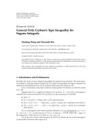
Figure 1: (a) 45-degree tilted form of the kernel with zeros filled
in to form the centrosymmetric matrix

Ψ, (b) eigensystem decom-
position of 90-degree rotated right upper quadrant of the kernel
matrix, corresponding to matrix R, with cartoon eigenvectors and
the impulse function (Step 2 in the algorithm), and (c) synthesis by
rotating back corresponding to Step 3 in the algorithm.
The modified eigendecomposition described above is
illustrated in Figure 1. This modified eigendecomposition
approach reduces the computational complexity by reducing
the number of spectrograms and using windows that are
shorter in length. In this paper, this approach will be used to

construct computationally efficient scale covariant kernels.
3. Scale Covariant Computationally
Efficient TFDs
The eigendecomposition algorithm described in the previous
section shows that the computation of any TFD can be
reduced to the computation of cross-spectrograms using
the eigenvectors of the kernel submatrix as the window
functions. In order to construct a scale covariant time-
frequency kernel, we first have to determine the corre-
sponding eigenvectors. In this section, we will determine
whether the eigenvectors of a scale covariant kernel have any
particular structure.
In order for the TFD to be scale covariant, the cross-
spectrograms that constitute the TFD should each be scale
covariant. This is a sufficient but not necessary condition.
The cross-spectrograms will be scale covariant as long as the
STFTs involved are scale covariant. Therefore, we want to
determine the eigenvectors such that the STFTs computed
using them as window functions are scale covariant. First,
we will find a condition on the eigenvectors such that
the corresponding STFTs are scale covariant. Then, we will
construct kernels using these eigenvectors. The following
proofs will be given in the continuous time domain since
exact scale covariance cannot be achieved in discrete-time
[10]. The results will then be extended for discrete-time for
purposes of implementation.
Theorem 1. The Short-Time Fourier Transform of a signal is
scale covariant if and only if the window function satisfies the
scale invariance property, that is, h(at)
= (1/


a)h(t) for a ∈
R.
Proof. If the window function is scale invariant, then for a
scaled signal
√
as(at), the STFT is
STFT
scaled
(t, ω) =

h(t −τ)
√
as(aτ)e
−jωτ
dτ
=
1
√
a

h

t −
τ

a

s


τ


e
−jωτ

/a
dτ

=
1
√
a

h

at −τ

a

s

τ


e
−jωτ

/a
dτ


=

h

at −τ


s

τ


e
−jωτ

/a
dτ

= STFT

at,
ω
a

,
(9)
where the second to last equality is obtained by the scale
invariance property of the window function h. The converse
canbeproveninasimilarmanner.

Now that we have shown that scale invariant window
functions produce scale covariant STFTs, we have to deter-
mine the class of window functions that satisfy this scale
invariance property.
Theorem 2. The only real function h(t) which sat isfies the
scale invariance property is K/
√
t,whereK ∈ R.
Proof. In order to find h(t) such that h(at)
= (1/
√
a)h(t), we
use the scale transform which is defined as [1]
D(c)
=
1
√
2π

∞
0
h(t)
e
−jc ln t
√
t
dt. (10)
If we take the scale transform of the two sides in the equality
h(at)
= (1/

√
a)h(t), we obtain
1
√
2π

∞
0
h(at)
e
−jc ln t
√
t
dt
=
1
√
a
D(c),
1
√
2π
1
√
a
e
jcln a

∞
0

h

t


e
−jc ln t

√
t

dt

=
1
√
a
D(c),
e
jcln a
D(c) = D(c).
(11)
The last equality is true when c
= 0. This implies that
D(c)
= 0, for c
/
=0. Therefore, the only real solution for D(c)
is Kδ(c), K
∈ R. By taking the inverse scale transform of

Kδ(c), we can obtain h(t) as follows:
h(t)
=

Kδ(c)
e
jcln t
√
t
dc
=
K
√
t
, t>0. (12)
3.1. Construction of a Scale Covariant Kernel. The discrete-
time equivalent of the scale invariant function K/
√
t is K/
√
n
for n
≥ 1. In order for the TFD computed by (8)tobescale
covariant, all of the window functions used in computing
the spectrograms should be of the form K/
√
n. This implies
4 EURASIP Journal on Advances in Signal Processing
that the eigenvectors Jx
i

and the vector z in (8) should all
be in this form. Since the vectors of the form K/
√
n are
linearly dependent, the kernel submatrix JB can have at
most one eigenvector Jx. Therefore, the scale covariant kernel
is constructed using a single eigenvector. We can generate
a family of scale covariant kernels using different values
for K.
In the following discussions, we will choose z(n)
=
K
1
/
√
n and Jx(n) = K
2
/
√
n.A2N +1× 2N +1kernel,

Ψ,
can be constructed using these two vectors based on (5)as
follows:

Ψ =
⎡
⎢
⎢
⎢

⎢
⎢
⎢
⎢
⎢
⎢
⎢
⎢
⎢
⎢
⎢
⎢
⎢
⎢
⎢
⎢
⎢
⎢
⎢
⎢
⎢
⎢
⎢
⎢
⎢
⎣
.
.
.
00

.
.
.
.
.
.
.
.
.
.
.
.
··· ··· 0
K
1
√
2
K
2
2
√
2
K
2
2
2
···
··· ···
0 K
1

K
2
2
K
2
2
√
2
···
···
K
1
√
2
K
1
1 K
1
K
1
√
2
···
···
K
2
2
√
2
K

2
2
K
1
0 ··· ···
···
K
2
2
2
K
2
2
√
2
K
1
√
2
0
··· ···
.
.
.
.
.
.
.
.
.

.
.
.00
.
.
.
⎤
⎥
⎥
⎥
⎥
⎥
⎥
⎥
⎥
⎥
⎥
⎥
⎥
⎥
⎥
⎥
⎥
⎥
⎥
⎥
⎥
⎥
⎥
⎥

⎥
⎥
⎥
⎥
⎥
⎦
. (13)
The only eigenvector of this matrix is [
11/
√
21/
√
31/2 ···
]
T
which is the scale invariant window function x(n) =
1/
√
n. Defining

δ = [
0
1×N
1 0
1×N
], x = [
0
1×N+1
x
], the

corresponding time-frequency distribution can be written as
follows:
TFD(n, ω)
= SP
z,

δ
(n, ω)+SP

δ,z
(n, ω)
+SP
Jz,

δ
(n, ω)+SP

δ,Jz
(n, ω)
+SP
x,Jx
(n, ω)+SP
Jx,x
(n, ω)+SP

δ,

δ
(n, ω)
= 2Re


SP
x,Jx
(n, ω)} +2Re{SP
z,

δ
(n, ω)

+2Re

SP
Jz,

δ
(n, ω)

+SP

δ
,

δ
(n, ω),
(14)
where SP corresponds to the cross-spectrogram using the
different window functions. Note that for this scale covariant
kernel, the vector z is the same as Jx up to a scalar constant.
Therefore, this representation relies on the computation of
one nontrivial STFT, the one computed using

x as the
window function. The other STFTs are trivial as in the case
of the impulse function or can be easily obtained from
this STFT by applying time reversal and amplitude scaling
operations.
3.2. Computational Complexity. The computational com-
plexity of this time-frequency distribution consists of com-
puting 3 distinct STFTs, one of which is trivial. Based on the
results in [5], the total number of real multiplications per
time-frequency point for a TFD with size 2N +1
×N
F
is given
as follows:
3+
3

N +(N/2)log
2
(N
F
/2) + (2/3)N
F

N
F
+ 4, (15)
where the first term corresponds to the 3 real multiplications
required for computing the spectrogram with the impulse
function; the second term corresponds to the computational

complexity of the cross-spectrograms computed using Jx
and x,eachofwhichrequiresN complex multiplications
between the window and the signal, an N point FFT, and
2N
F
real multiplications for multiplying with the complex
conjugate; the third term corresponds to the computational
complexity of multiplying the STFTs computed using the
impulse function and J
z or z. Therefore, the total compu-
tational complexity is in the order of O(log N)compared
to O(N
2
log N) for bilinear time-frequency distributions
belonging to Cohen’s class with a nontrivial kernel function,
that is, excluding the Wigner distribution.
3.3. Properties. In this section, some properties of the
proposed scale covariant, computationally efficient kernel
will be discussed.
(1) Time Marginal. This kernel will satisfy the time marginal
since ψ(n,0)
= δ(n) by construction (see (13)).
(2) Frequency Marginal. This kernel will not satisfy the
frequency marginal since

n
ψ(n, m)
/
=1 ∀m. (16)
(3) Reduced Interference Distribut ion. Reduced interference

is a desired property for bilinear time-frequency distri-
butions especially in the case of multicomponent signals
where cross-terms contaminate the representation. Reduced
interference distribution requires the kernel φ(θ, m)todecay
as we move away from the θ, m axis. This condition implies
that the kernel is smoothly decaying, that is, ψ(n, m) should
also be smoothly decaying as n increases. In our case, the
kernel is given by
ψ(n, m)
=
⎧
⎪
⎪
⎪
⎪
⎪
⎪
⎨
⎪
⎪
⎪
⎪
⎪
⎪
⎩
1, n = 0, m = 0,
K
2
2




n + m/2



|n −m/2|
, |n| <
|m|
2
,
K
1

|n| + |m|/2
,
|n|=
|
m|
2
,
(17)
whichdecaysasafunctionofn.
4. Experimental Results
In this section, two examples will be given to illustrate the
scale covariance and reduced interference properties of the
proposed distribution.
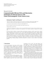
4.1. Example 1: Evaluation of the Scale Covariance. Let s be a
signal that consists of the sum of two Gabor logons, where
the Gabor logons are the time-shifted and -scaled versions of

EURASIP Journal on Advances in Signal Processing 5
0
0.1
0.2
0.3
0.4
0.5
0.6
0.7
0.8
0.9
1
Normalized frequency
20 40 60 80 100 120
Time samples
(a)
0
0.1
0.2
0.3
0.4
0.5
0.6
0.7
0.8
0.9
1
Normalized frequency
20 40 60 80 100 120
Time samples

(b)
30
25
20
15
10
5
Scale
20 40 60 80 100 120
Time samples
(c)
Figure 2: Scale covariant distribution for a Gabor logon and its time-scaled version. (a) Scale covariant distribution, (b) Wigner distribution,
and (c) Wavelet distribution using the Morlet wavelet.
0
0.1
0.2
0.3
0.4
0.5
0.6
0.7
0.8
0.9
1
Normalized frequency
50 100 150 200 250
Time samples
(a)
0
0.1

0.2
0.3
0.4
0.5
0.6
0.7
0.8
0.9
1
Normalized frequency
50 100 150 200 250
Time samples
(b)
0
0.1
0.2
0.3
0.4
0.5
0.6
0.7
0.8
0.9
1
Normalized frequency
50 100 150 200 250
Time samples
(c)
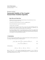
Figure 3: Time-frequency distribution for two crossing chirp signals. (a) Scale covariant distribution, (b) Wigner distribution, and (c)
Reduced interference distribution using the Born-Jordan kernel.

each other, that is, s(n) = exp(−(n −n
0
)
2
/σ)exp(−j2π(n −
n
0
)k
0
)+exp(−(n − n
1
)
2
/aσ)exp(−j2π(n−n
1
)k
0
). The time-
frequency kernel is constructed as described in the previous
section using K
1
= K
2
= 0.5, that is, z(n) = Jx(n) = 1/2
√
n.
Figure 2 compares the time-frequency representations of this
signal for three different distributions: the computational
efficient scale covariant distribution introduced in this paper,
the Wigner distribution, and the wavelet transform using the

Morlet wavelet. It can be seen that the Wigner distribution
and the scale covariant distribution are similar to each other.
Both of these representations scale in time and frequency
according to the time scaling factor a, with the difference
being the resolution. Wigner distribution achieves higher
resolution than the scale covariant kernel since it is based
on computing cross-spectrograms using multiple windows
rather than a single window. When the scale covariant
distribution is compared to the wavelet transform, it can be
seen that wavelet transform scales in time and frequency at
the expense of reduced resolution. This reduced resolution
is due to the fact that the wavelet transform has constant-
Q resolution, that is, at low frequencies it provides high-
frequency resolution and low-time resolution, whereas at
high frequencies the opposite is true. Therefore, the class of
scale covariant distributions proposed in this paper satisfies
several desired properties such as high time-frequency reso-
lution, scale covariance, and low computational complexity,
simultaneously.
4.2. Example 2: Evaluation of the Cross-Terms. In this
example, we compare the proposed scale covariant time-
frequency distribution to the Wigner distribution and a
reduced interference distribution (Born-Jordan distribution)
in terms of the amount of cross-terms. For this purpose, we
consider the sum of two chirp signals, x(t)
= exp(j(ω
1
t +
β
1

t
2
)) + exp(j(ω
2
t + β
2
t
2
)), where ω
2
= ω
1
+ β
1
t
final
and β
2
=
−
β
1
. The time-frequency kernel is constructed as described
in the previous example using K
1
= K
2
= 0.5, that is, z(n) =
Jx(n) = 1/2
√

n. The three time-frequency distributions
obtained using the three different kernel functions are shown
in Figure 3. We quantify the amount of cross-terms in the
different TFDs using a signal-to-noise ratio (SNR) type
measure in the time-frequency plane as follows:
SNR
= 10 log

n

k
TFD
2
auto-terms
(n, k)

n

k
TFD
2
cross-terms
(n, k)
, (18)
which measures the ratio of the energy of the autoterms to
the energy of the cross-terms. The SNR for the three distri-
butions are 0.0363 dB for Wigner distribution, 2.6643 dB for
scale covariant distribution, and 3.1528 dB for Born-Jordan
distribution. As we can see from the actual distributions
and the SNRs, the proposed scale covariant distribution is

better in terms of suppressing the cross-terms compared
to the Wigner distribution. The proposed distribution
also has lower computational complexity than Born-Jordan
6 EURASIP Journal on Advances in Signal Processing
distribution at the expense of a slight increase in the energy
of the cross-terms. Therefore, the proposed distribution
achieves a tradeoff between the Wigner distribution and the
general class of reduced interference distributions in terms of
computational complexity and the amount of cross-terms.
5. Conclusions
In this paper, we introduced a new method for constructing
scale covariant time-frequency distributions. It is shown
that the scale covariant kernels can be constructed using a
single scale invariant eigenvector combined with the impulse
function. This realization leads to a computationally efficient
TFD computation algorithm where the TFD is composed of
three short-time Fourier transforms, of which only one is
nontrivial and distinct. The resulting distribution is shown
to be scale covariant. Comparisons with other well-known
scale covariant representations show that the proposed
distribution achieves scale covariance simultaneously with
low computational complexity, high-frequency resolution,
and reduced interference.
References
[1] L. Cohen, Time-Frequency Analysis, Prentice-Hall, Englewood
Cliffs, NJ, USA, 1995.
[2] C. S. Burrus, R. A. Gopinath, and H. Guo, Introduction to
Wavelets and Wavelet Transforms, Prentice-Hall, Englewood
Cliffs, NJ, USA, 1997.
[3] J. Bertrand and P. Bertrand, “A class of affine Wigner functions

with extended covariance properties,” Journal of Mathematical
Physics, vol. 33, no. 7, pp. 2515–2527, 1992.
[4] A. Papandreou, F. Hlawatsch, and G. F. Boudreaux-
Bartels, “The hyperbolic class of quadratic time-frequency
representations—part I: constant-Q warping, the hyperbolic
paradigm, properties, and members,” IEEE Transactions on
Signal Processing, vol. 41, no. 12, pp. 3425–3444, 1993.
[5] S. Aviyente and W. J. Williams, “A centrosymmetric kernel
decomposition for time-frequency distribution computation,”
IEEE Transactions on Signal Processing, vol. 52, no. 6, pp. 1574–
1584, 2004.
[6] G. S. Cunnigham and W. J. Williams, “Kernel decomposition
of time-frequency distributions,” IEEE Transactions on Signal
Processing, vol. 42, no. 6, pp. 1425–1442, 1994.
[7] J. Jeong and W. J. Williams, “Alias-free generalized discrete-
time time-frequency distributions,” IEEE Transactions on
Signal Processing, vol. 40, no. 11, pp. 2757–2765, 1992.
[8] M. G. Amin, “Spectral decomposition of time-frequency
distribution kernels,” IEEE Transactions on Signal Processing,
vol. 42, no. 5, pp. 1156–1165, 1994.
[9] A. Cantoni and P. Butler, “Eigenvalues and eigenvectors of
symmetric centrosymmetric matrices,” Linear Algebra and Its
Applications, vol. 13, no. 3, pp. 275–288, 1976.
[10] E. J. Zalubas, Signal processing and pattern recognition in
scale-content domains: theory and applications, Ph.D. thesis,
University of Michigan, Ann Arbor, Mich, USA, 1999.