Báo cáo hóa học: " Research Article A Perceptually Relevant No-Reference Blockiness Metric Based on Local Image Characteristics Hantao Liu (EURASIP Member)1 and Ingrid " potx

Hindawi Publishing Corporation
EURASIP Journal on Advances in Signal Processing
Volume 2009, Article ID 263540, 14 pages
doi:10.1155/2009/263540
Research Article
A Perceptually Relevant No-Reference Blockiness Metric Based on
Local Image Characteristics
Hantao Liu (EURASIP Member)
1
andIngridHeynderickx
1, 2
1
Department of Mediamatics, Delft University of Technology, 2628 CD Delft, The Netherlands
2
Group Visual Expe riences, Philips Research Laboratories, 5656 AA Eindhoven, The Netherlands
Correspondence should be addressed to Hantao Liu,
Received 4 July 2008; Revised 20 December 2008; Accepted 21 January 2009
Recommended by Dimitrios Tzovaras
A novel no-reference blockiness metric that provides a quantitative measure of blocking annoyance in block-based DCT coding
is presented. The metric incorporates properties of the human visual system (HVS) to improve its reliability, while the additional
cost introduced by the HVS is minimized to ensure its use for real-time processing. This is mainly achieved by calculating the local
pixel-based distortion of the artifact itself, combined with its local visibility by means of a simplified model of visual masking. The
overall computation efficiency and metric accuracy is further improved by including a grid detector to identify the exact location
of blocking artifacts in a given image. The metric calculated only at the detected blocking artifacts is averaged over all blocking
artifacts in the image to yield an overall blockiness score. The performance of this metric is compared to existing alternatives in
literature and shows to be highly consistent with subjective data at a reduced computational load. As such, the proposed blockiness
metric is promising in terms of both computational efficiency and practical reliability for real-life applications.
Copyright © 2009 H. Liu and I. Heynderickx. This is an open access article distributed under the Creative Commons Attribution
License, which permits unrestricted use, distribution, and reproduction in any medium, provided the original work is properly
cited.
1. Introduction

Objective metrics, which serve as computational alternatives
for expensive image quality assessment by human sub-
jects, aimed at predicting perceived image quality aspects
automatically and quantitatively. They are of fundamental
importance to a broad range of image and video processing
applications, such as for the optimization of video coding
or for real-time quality monitoring and control in displays
[1, 2]. For example, in the video chain of current TV-
sets, various objective metrics, which determine the quality
of the incoming signal in terms of blockiness, ringing,
blur, and so forth and adapt the parameters in the video
enhancement algorithms accordingly, are implemented to
enable an improved overall perceived quality for the viewer.
In the last decades, a considerable amount of research
has been carried out on developing objective image quality
metrics, which can be generally classified into two categories:
full-reference (FR) metrics and no-reference (NR) metrics
[1]. The FR metrics are based on measuring the similarity or
fidelity between the distorted image and its original version,
which is considered as a distortion-free reference. However,
in real-world applications the reference is not always fully
available; for example, the receiving end of a digital video
chain usually has no access to the original image. Hence,
objective metrics used in these types of applications are
constrained to a no-reference approach, which means that
the quality assessment relies on the reconstructed image
only. Although human observers can easily judge image
quality without any reference, designing NR metrics is still an
academic challenge mainly due to the limited understanding
of the human visual system [1]. Nevertheless, since the

structure information of various image distortions is well
known, NR metrics designed for specific quality aspects
rather than for overall image quality are simpler, and
therefore, more realistic [2].
Since the human visual system (HVS) is the ultimate
assessor of most visual information, taking into account the
way human beings perceive quality aspects, while removing
perceptual redundancies, can be greatly beneficial for match-
ing objective quality prediction to human, perceived quality
[3]. This statement is adequately supported by the observed
2 EURASIP Journal on Advances in Signal Processing
shortcoming of the purely pixel-based metrics, such as the
mean square error (MSE) and peak signal-to-noise ratio
(PSNR). They insufficiently reflect distortion annoyance to
the human eye, and thus often exhibit a poor correlation
with subjective test results (e.g., in [1]). The performance
of these metrics has been enhanced by incorporating certain
properties of the HVS (e.g., in [4–7]). But since the HVS is
extremely complex, an objective metric based on a model of
the HVS often is computationally very intensive. Hence, to
ensure that an HVS-based objective metric is applicable to
real-time processing, investigations should be carried out to
reduce the complexity of the HVS model as well as of the
metric itself without significantly compromising the overall
performance.
One of the image quality distortions for which several
objective metrics have been developed is blockiness. A
blocking artifact manifests itself as an artificial discontinuity
in the image content and is known to be the most annoying
distortion at low bit-rate DCT coding [8]. Most objective

quality metrics either require a reference image or video (e.g.,
in [5–7]), which restricts their use in real-life applications,
or lack an explicit human vision model (e.g., in [9, 10]),
which limits their reliability. Apart from these metrics, no-
reference, blockiness metrics, including certain properties
of the HVS are developed. Recently, a promising approach,
which we refer to as feature extraction method, is proposed
in [11, 12], where the basic idea is to extract certain image
features related to the blocking artifact and to combine
them in a quality prediction model with the parameters
estimated from subjective test data. The stability of this
method, however, is uncertain since the model is trained with
a limited set of images only, and its reliability to other images
is not proved yet.
A no-reference blockiness metric can be formulated
either in the spatial domain or in the transform domain. The
metrics described, for example, in [13, 14] are implemented
in the transform domain. In [13], a 1-D absolute difference
signal is combined with luminance and texture masking,
and from that blockiness is estimated as the peaks in the
power spectrum using FFT. In this case, the FFT has to be
calculated many times for each image, which is therefore very
expensive. The algorithm in [14] computes the blockiness as
a result of a 2-D step function weighted with a measure of
local spatial masking. This metric requires the access to the
DCT encoding parameters, which are, however, not always
available in practical applications.
In this paper, we rely on the spatial domain approach.
The generalized block-edge impairment metric (GBIM) [15]
is the most well-known metric in this domain. GBIM

expresses blockiness as the interpixel difference across block
boundaries scaled with a weighting function, which simply
measures the perceptual significance of the difference due
to local spatial masking of the HVS. The total amount of
blockiness is then normalized by the same measure calcu-
lated for all other pixels in an image. The main drawbacks
for GBIM are (1) the interpixel difference characterizes the
block discontinuity not to the extent that local blockiness is
sufficiently reliably predicated; (2) the HVS model includes
both luminance masking and texture masking in a single
weighting function, and efficient integration of different
masking effects is not considered, hence, applying this model
in a blockiness metric may fail in assessing demanding
images; (3) the metric is designed such that the human
visionmodelneedstobecalculatedforeverypixelinan
image, which is computationally very expensive. A second
metric using the spatial domain is based on a locally adaptive
algorithm [16] and is hereafter referred to as LABM. It
calculates a blockiness metric for each individual coding
block in an image and simultaneously estimates whether
the blockiness is strong enough to be visible to the human
eye by means of a just-noticeable-distortion (JND) profile.
Subsequently, the local metric is averaged over all visible
blocks to yield a blockiness score. This metric is promising
and potentially more accurate than GBIM. However, it
exhibits several drawbacks: (1) the severity of blockiness for
individual artifacts might be under- or overestimated by
providing an averaged blockiness value for all artifacts within
this block; (2) calculating an accurate JND profile which
provides a visibility threshold of a distortion due to masking

is complex, and it cannot predict perceived annoyance above
threshold; (3) the metric needs to estimate the JND for every
pixel in an image, which largely increases the computational
cost.
Calculating the blockiness metric only at the expected
block edges, and not at all pixels in an image, strongly reduces
the computational power, especially when a complex HVS is
involved. To ensure that the metric is calculated at the exact
position of the block boundaries, a grid detector is needed
since in practice deviations in the blocking grid might occur
in the incoming signal, for example, as a consequence of
spatial scaling [9, 17, 18]. Without this detection phase, no-
reference metrics might turn out to be useless, as blockiness
is calculated at wrong pixel positions.
In this paper, a novel algorithm is proposed to quantify
blocking annoyance based on its local image characteristics.
It combines existing ideas in literature with some new
contributions: (1) a refined pixel-based distortion measure
for each individual blocking artifact in relation to its direct
vicinity; (2) a simplified and more efficient visual masking
model to address the local visibility of blocking artifacts
to the human eye; (3) the calculation of the local pixel-
based distortion and its visibility on the most relevant
stimuli only, which significantly reduces the computational
cost. The resulting metric yields a strong correlation with
subjective data. The rest of the paper is organized as follows.
Section 2 details the proposed algorithm, Section 3 provides
and discusses the experimental results, and the conclusions
are drawn in Section 4.
2. Description of the Algorithm

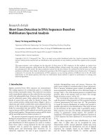
The schematic overview of the proposed approach is illus-
trated in Figure 1 (the first outline of the algorithm was
already described in [19]). Initially, a grid detector is adopted
in order to identify the exact position of the blocking
artifacts. After locating the artifacts, local processing is
carried out to individually examine each detected blocking
artifact by analyzing its surrounding content to a limited
EURASIP Journal on Advances in Signal Processing 3
Input
image
Blocking grid
detector
Local blockiness
metric
Averaging
NPBM
Local pixel-based
blockiness
Local visibility
Image
database
LPB VC
LBM
Figure 1: Schematic overview of the proposed approach.
extent. This local calculation consists of two parallel steps:
(1) measuring the degree of local pixel-based blockiness
(LPB); (2) estimating the local visibility of the artifact to the
human eye and outputting a visibility coefficient (VC). The
resulting LPB and VC are integrated into a local blockiness
metric (LBM). Finally, the LBM is averaged over the blocking

grid of the image to produce an overall score of blockiness
assessment (i.e., NPBM). The whole process is calculated
on the luminance channel only in order to further reduce
the computational load. The algorithm is performed for the
blockiness once in horizontal direction (i.e., NPBM
h
)and
once in vertical direction NPBM
v
. From both values, the
average is calculated assuming that the human sensitivity to
horizontal and vertical blocking artifacts is equal.
2.1. Blocking Grid Detection. Since the arbitrary grid prob-
lem has emerged as a crucial issue especially for no-reference
blockiness metrics, where no prior knowledge on grid
variation is available, a grid detector is required in order
to ensure a reliable metric [9, 18]. Most, if not all, of the
existing blockiness metrics make the strong assumption that
the grid exists of blocks: 8
× 8 pixels, starting exactly at the
top-left corner of an image. However, this is not necessarily
the case in real-life applications. Every part of a video chain,
from acquisition to display, may induce deviations in the
signal, and the decoded images are often scaled before being
displayed. As a result, grids are shifted, and the block size is
changed.
Methods, as, for example, in [13, 17] employ a frequency-
based analysis of the image to detect the location of blocking
artifacts. These approaches, due to the additional signal
transform involved, are often computationally inefficient.

Alternatives in the spatial domain can be found in [9, 18].
They both map an image into a one-dimensional signal
profile. In [18], the block size is estimated using a rather
complex maximum-likelihood method, and the grid offset
is not considered. In [9], the block size and the grid offset
are directly extracted from the peaks in the 1-D signal by
calculating the normalized gradient for every pixel in an
image. However, spurious peaks in the 1-D signal as a result
of edges from objects may occur and consequently yield
possible detection errors. In this paper, we further rely on the
basic ideas of both [9, 18], but implement them by means of a
simplified calculation of the 1-D signal and by extracting the
block size and the grid offset using DFT of the 1-D signal.
The entire procedure is performed once in horizontal and
once in vertical directions to address a possible asymmetry
in the blocking grid.
2.1.1. 1-D Sig nal Ext raction. Since blocking artifacts reg-
ularly manifest themselves as spatial discontinuities in an
image, their behavior can be effectively revealed through a
1-D signal profile, which is simply formed calculating the
gradient along one direction (e.g., horizontal direction) and
then summing up the results along the other direction (e.g.,
vertical direction). We denote the luminance channel of an
image signal of M
× N (height × width) pixels as I(i, j)for
i
∈ [1, M], j ∈ [1, N], and calculate the gradient map G
h
along the horizontal direction
G

h
(i, j) =|I(i, j +1)−I(i, j)|, j ∈ [1, N −1]. (1)
The resultant gradient map is reduced to a 1-D signal
profile S
h
by summing G
h
along the vertical direction
S
h
(j) =
M

i=1
G
h
(i, j). (2)
2.1.2. Block Size Ext raction. Based on the fact that the
amount of energy present in the gradient at the borders
4 EURASIP Journal on Advances in Signal Processing
of coding blocks is greater than that in the intermediate
positions blocking artifacts, if existing, are present as a
periodic impulse train of signal peaks. These signal peaks
can be further enhanced using some form of spatial filtering,
which makes the peaks stand out from their vicinity. In
this paper, a median filter is used. Then a promoted 1-D
signal profile PS
h
is obtained simply subtracting from S
h

its
median-filtered version MS
h
:
PS
h
(j) = S
h
(j) −MS
h
(j),
MS
h
(j) = Median

S
h
(j − k), , S
h
(j), , S
h
(j + k)

,
(3)
where the size of the median filter (2k + 1) depends on N.
In our experiments, N is, for example, 384, and then k is
4. The resulting 1-D signal profile PS
h
intrinsically reveals

the blocking grid as an impulse train with a periodicity
determined by the block size. However, in demanding
conditions, such as for images with many object edges, the
periodicity in the regular impulses might be masked by noise
as a result of image content. This potentially makes locating
the required peaks and estimating their periodicity more
difficult. The periodicity of the impulse train, corresponding
to the block size, is more easily extracted from the 1-D
signal PS
h
in the frequency domain using the discrete Fourier
transform (DFT).
2.1.3. Grid Offset Extraction. After the block size (i.e., p)is
determined, the offset of the blocking grid can be directly
retrieved from the signal PS
h
, in which the peaks are located
at multiples of the block size. Thus, a simple approach based
on calculating the accumulative value of grid peaks with a
possible offset Δx (e.g., Δx
= 0:(p − 1) with the periodic
feature in mind) is proposed. For each possible offset value
Δx, the accumulator is defined as
A(Δx)
=
[N/p]−1

i=1
PS
h

(Δx + p · i), Δx ∈ [0, p −1]. (4)
The offset is determined as
A(Δx)
= MAX [ A(0) ···A(p −1) ]. (5)
Based on the results of the block size and grid offset,
the exact position of blocking artifacts can be explicitly
extracted.
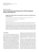
2.1.4. An Example. A simple example is given in Figure 2,
where the input image “bikes” of 128
× 192pixelsisJPEG-
compressed using a standard block size of 8
× 8 pixels. The
displayed image is synthetically upscaled with a scaling factor
2
× 2 and shifted by 8 pixels both from left to right and
from top to bottom. As a result, the displayed image size is
256
× 384 pixels, the block size 16 × 16 pixels, and the grid
starts at pixel position (8, 8) instead of at the origin (0, 0), as
shown in Figure 2(a). The proposed algorithm toward a 1-D
signal profile is illustrated in Figure 2(b). Figure 2(c) shows
the magnitude profile of the DFT applied to the signal PS.
It allows extraction of the period p (i.e., p
= 1/0.0625 = 16
pixels), which is maintained over the whole frequency range.
Based on the detected block size p
= 16, the grid offset
is calculated as Δx
= 8. Then the blocking grid can be
determined, as shown in Figure 2(d).

2.2. Local Pixel-Based Blockiness Measure. Since blocking
artifacts intrinsically are a local phenomenon, their behavior
can be reasonably described at a local level, indicating the
visual strength of a distortion within a local area of image
content. Based on the physical structure of blocking artifacts
as a spatial discontinuity, this can be simply accomplished
relating the energy present in the gradient at the artifact
with the energy present in the gradient within its vicinity.
This local distortion measure (LDM) purely based on pixel
information can be formulated as
LDM(k)
=
E
k
(i, j)
f

E
V(k)
(i, j)

, k = 1, , n,(6)
where f [
·] indicates the pooling function, for example,
Σ, mean,orL2-norm,E
k
indicates the gradient energy
calculated for each individual artifact, E
V(k)
indicates the

gradient energy calculated at the pixels in the direct vicinity
of this artifact, and n is the total number of blocking artifacts
in an image. Since the visual strength of a block discontinuity
is primarily affected by its local surroundings of limited
extent, this approach is potentially more accurate than a
global measure of blockiness (e.g., [9, 15]), where the overall
blockiness is assessed by the ratio of the averaged disconti-
nuities on the blocking grid and the averaged discontinuities
in pixels which are not on the blocking grid. Furthermore,
the local visibility of a distortion due to masking can now be
easily incorporated, with the result that it is only calculated
at the location of the blocking artifacts. This means that
modeling the HVS on nonrelevant pixels is eliminated as
compared to the global approach (e.g., [15]).
In this paper, we rely on the interblock difference defined
in [16] and extend the idea by reducing the dimension of
the blockiness measure from a signal block to an individual
blocking artifact. As such, the local distortion measure
(LDM) is implemented on the gradient map, resulting in
local pixel-based blockiness (LPB). The LPB quantifies the
blocking artifact at pixel location (i, j)as
LPB
h
(i, j) =
⎧
⎪
⎪
⎪
⎨
⎪

⎪
⎪
⎩
ω ×BG
h
if NBG
h
= 0, BG
h
/
=0,
BG
h
NBG
h
if NBG
h
/
=0,
0ifNBG
h
= 0, BG
h
= 0,
(7)
where BG
h
and NBG
h
are

BG
h
= G
h
(i, j),
NBG
h
=
1
2n

x=−n, ,n,x
/
=0
G
h
(i, j + x).
(8)
The definition of the LPB is further explained as follows:
(1) The template addressing the direct vicinity is defined
as a 1-D element including n adjacent pixels to the
EURASIP Journal on Advances in Signal Processing 5
Grid origin: (0, 0)
Block size: 8
×8
Grid origin: (8, 8)
Block size: 16
×16
(a) Input image (left) and displayed image (right)
S

10000
5000
0
MS
3000
2000
1000
0
PS
6000
4000
2000
0
50 100 150 200 250 300 350
50 100 150 200 250 300 350
50 100 150 200 250 300 350
(b) 1-D signal formation: S, MS and PS are calculated according to (2)
and (3) for the displayed image in (a) along the horizontal direction
DFT magnitudes
1
0.9
0.8
0.7
0.6
0.5
0.4
0.3
0.2
0.1
0

Frequency (1/N )
00.05 0.10.15 0.20.25 0.30.35 0.40.45 0.5
X :0.0625
Y :0.4302
(c) DFT magnitudes of PS in (b)
PS
6000
4000
2000
0
50 100 150 200 250 300 350
(d) Blocking grid detected from the displayed image in (a) along the
horizontal direction
Figure 2: Blocking grid detection: an example.
left and to the right of an artifact. The size of the
template (2n + 1) is designed to be proportional to
the detected block size p (e.g., n
= p/2), taking into
account possible scaling of the decoded images. An
example of the template is shown in Figure 3,where
two adjacent 8
×8 blocks (i.e., A and B) are extracted
from a real JPEG image.
(2) BG
h
denotes the local energy present in the gradient
at the blocking artifact, and NBG
h
denotes the
averaged gradient energy over its direct vicinity. If

NBG
h
= 0, only the value of BG
h
determines the
local pixel-based blockiness. In this case, LPB
h
= 0
(i.e., BG
h
= 0) means there is no block discontinuity
appearing, and the blocking artifact is spurious.
LPB
h
= ω × BG
h
(i.e., BG
h
/
=0) means the artifact
exhibits a severe extent of blockiness, and ω (ω
= 1
in our experiments) is used to adjust the amount of
gradient energy. If NBG
h
/
=0, the local pixel-based
blockiness is simply calculated as the ratio of BG
h
over NBG

h
.
Image domain I Gradient domain G
h
Location of blocking artifacts
AB
Figure 3: Local pixel-based blockiness (LPM).
(3) The local pixel-based blockiness LPB
h
is specified in
(7)to(8) for a block discontinuity along the hor-
izontal direction. The measure of LPB
v
for vertical
blockiness can be easily defined in a similar way. The
calculation is then performed within a vertical 1-D
template.
2.3. Local Visibility Estimat ion. To predict perceived quality,
objective metrics based on models of the human visual
system are potentially more reliable [3, 20]. However, from
6 EURASIP Journal on Advances in Signal Processing
a practical point of view, it is highly desirable to reduce
the complexity of the HVS model without compromising
its abilities. In this paper, a simplified human vision model
based on the spatial masking properties of the HVS is
proposed. It adopts two fundamental characteristics of
the HVS, which affect the visibility of an artifact in the
spatial domain: (1) the averaged background luminance
surrounding the artifact; (2) the spatial nonuniformity in
the background luminance [20, 21]. They are known as

luminance masking and texture masking, respectively, and
both are highly relevant to the perception of blocking
artifacts.
Various models of visual masking to quantify the vis-
ibility of blocking artifacts in images have been proposed
in literature [7, 11, 15, 21, 22]. Among these models, there
are two widely used ones: the model used in GBIM [15]
and the just-noticeable-distortion (JND) profile model used
in [21]. Their disadvantages have already been pointed out
in Section 1. Our proposed model is illustrated in Figure 4.
Both texture and luminance masking are implemented by
analyzing the local signal properties within a window,
representing the local surrounding of a blocking artifact.
A visibility coefficient as a consequence of masking (i.e.,
VC
t
and VC
l
, resp.) is calculated using spatial filtering
followed by a weighting function. Then, both coefficients
are efficiently combined into a single visibility coefficient
(VC), which reflects the perceptual significance of the artifact
quantitatively.
2.3.1. Local Visibility Due to Texture Masking. Figure 5 shows
an example of texture masking on blocking artifacts, where
“a” and “b” are patterns including 4 adjacent blocks of 8
× 8
pixels extracted from a JPEG-coded image. As can be seen
from the right-hand side of Figure 5, pattern “a” and pattern
“b” both intrinsically exhibit block discontinuities. However,

as shown on the left-hand side of Figure 5, the block
discontinuities in pattern “b” are perceptually masked by its
nonuniform background, while the block discontinuities in
pattern “a” are much more visible as it is in a flat background.
Therefore, texture masking can be estimated from the local
background activity [20]. In this paper, texture masking is
modeled calculating a visibility coefficient (VC
t
), indicating
the degree of texture masking. The higher the value of this
coefficient, the smaller the masking effect, and hence, the
stronger the visibility of the artifact is. The procedure of
modeling texture masking comprises three steps.
(i) Texture detection: calculate the local background
activity (nonuniformity).
(ii) Thresholding: a classification scheme to capture the
active background regions.
(iii) Visibility transform function (VTF): obtain a visibil-
ity coefficient (VC
t
) based on the HVS characteristics
for texture masking.
Texture detection can be performed convolving the signal
with some form of high-pass filter. One of the Laws’ texture
energy filters [23] is employed here in a slightly modified
form. As shown in Figure 6, T1andT2 are used to measure
the background activity in horizontal and vertical directions,
respectively. A predefined threshold Thr (Thr
= 0.15 in our
experiments) is applied to classify the background into “flat”

or “texture,” resulting in an activity value I
t
(i, j), which is
given by
I
t
(i, j) =

0ift(i, j) < Thr,
t(i, j) otherwise,
(9)
t(i, j)
=
1
48
5

x=1
5

y=1
I(i −3+x, j − 3+y) ·T(x, y)
, (10)
where I(i, j) denotes the pixel intensity at location (i, j), T is
chosen as T1 for texture calculation in horizontal direction,
and T2 in vertical direction. It should be noted that splitting
up the calculation in horizontal and vertical directions, and
using a modified version of the texture energy filter, in which
some template coefficients are removed, can be done having
the application of a blockiness metric in mind. The texture

filters need to be adopted in case of extending these ideas to
other objective metrics.
A visibility transform function (VTF) is proposed in
accordance to human perceptual properties, which means
that the visibility coefficient VC
t
(i, j) is inversely propor-
tional (nonlinear) to the activity value I
t
(i, j). Figure 6 shows
an example of such a transform function, which can be
defined as
VC
t
(i, j) =
1

1+I
t
(i, j)

α
, (11)
where VC
t
(i, j) = 1, when the stimulus is in a “flat”
background, and α>1(α>5 in our experiments) is
used to adjust the nonlinearity. This shape of the VTF is an
approximation, considered to be good enough.
2.3.2. Local Visibility due to Luminance Masking. In many

psychovisual experiments, it was found that the human
visual system’ sensitivity to variations in luminance depends
on (is a nonlinear function of) the local mean luminance [7,
20, 21, 24]. Figure 7 shows an example of luminance masking
on blocking artifacts, where “a” and “b” are synthetic
patterns, each of which includes 2 adjacent blocks with
different gray-scale levels. Although the intensity difference
between the two blocks is the same in both patterns, the block
discontinuity of pattern “b” is much more visible than that in
pattern “a” due to the difference in background luminance.
In this paper, luminance masking is modeled based on two
empirically driven properties of the HVS: (1) a distortion
in a dark surrounding tends to be less visible than one in
a bright surrounding [7, 21] and (2) a distortion is most
visible for a surrounding with an averaged luminance value
between 70 and 90 (centered approx. at 81) in 8 bits gray-
scale images [24]. The procedure of modeling luminance
masking consists of two steps.
(i) Local luminance detection: calculate the local-
averaged background luminance.
(ii) Visibility transform function (VTF): obtain a visibil-
ity coefficient (VC
l
) based on the HVS characteristics
for luminance masking.
EURASIP Journal on Advances in Signal Processing 7
Texture masking
HPF VTF
t
VC

t
LPF VTF
1
VC
1
Luminance masking
Integration
strategy
VC
Figure 4: Schematic overview of the proposed human vision model.
a
b
Figure 5: An example of texture masking on blocking artifacts.
The local luminance of a certain stimulus is calculated
using a weighted low-pass filter as shown in Figure 8,in
which some template coefficients are set to “0.” The local
luminance I
l
(i, j)isgivenby
I
l
(i, j) =
1
26
5

x=1
5

y=1

I(i −3+x, j − 3+y) ·L(x, y), (12)
where L is chosen as L1 for calculating the background lumi-
nance in horizontal direction and L2 in vertical direction.
Again, splitting up the calculation in horizontal and vertical
directions, and using a modified low-pass filter, in which
some template coefficients are set to 0, is done with the
application of a blockiness metric in mind.
For simplicity, the relationship between the visibility
coefficient VC
l
(i, j) and the local luminance I
l
(i, j)ismod-
eled by a nonlinear function (e.g., power law) for low-
background luminance (i.e., below 81) and is approximated
by a linear function at higher background luminance (i.e.,
above 81). This functional behavior is shown in Figure 8 and
mathematically described as
VC
l
(i, j)=
⎧
⎪
⎪
⎪
⎪
⎨
⎪
⎪
⎪

⎪
⎩

I
l
(i, j)
81

1/2
if 0 ≤ I
l
(i, j) ≤ 81,

1−β
174

·

81−I
l
(i, j)

+1 otherwise,
(13)
where VC
l
(i, j) achieves the highest value of 1 when I
l
(i, j) =
81, and 0 <β<1(β = 0.7 in our experiments) is used to

adjust the slope of the linear part of this function.
2.3.3. Integration Strategy. The visibility of an artifact
depends on various masking effects coexisting in the HVS.
How to efficiently integrate them is an important issue in
obtaining an accurate perceptual model [25]. Since masking
intrinsically is a local phenomenon, the locality in the
visibility of a distortion due to masking is maintained in the
integration strategy of both masking effects. The resulting
approach is schematically given in Figure 9. Based on the
local image content surrounding a blocking artifact first the
texture masking is calculated. In case the local activity in the
area is larger than a given threshold (see (9)), a visibility
coefficient VC
t
is applied, followed by the application of a
luminance masking coefficient VC
l
. In case the local activity
in the area is low, only VC
l
is applied. The application of VC
l
,
where appropriately combined with VC
t
, results in an output
value VC.
2.4. The Perceptual Blockiness Metric. The local pixel-based
blockiness (LPB) defined in Section 2.2 is purely signal based
and so does not necessarily yield perceptually consistent

results. The human vision model proposed in Section 2.3
aims at removing the perceptually insignificant components
due to visual masking. Integration of these two elements can
be simply performed at a local level using the output of the
human vision model (VC) as a weighting coefficient to scale
the local pixel-based blockiness (LPB), resulting in a local
perceptual blockiness metric (LPBM). Since the horizontal
and vertical blocking artifacts are calculated separately, the
LPBM for the block discontinuity along the horizontal
direction is described as
LPBM
h
(i, j) = VC(i, j) ×LPB
h
(i, j), (14)
which is then averaged over all detected blocking artifacts in
the entire image to determine an overall blockiness metric,
that is, a no-reference perceptual blockiness metric (NPBM)
NPBM
h
=
1
n
n

k=1

LPBM
h
(i, j)


k
, (15)
where n is the total number of pixels on the blocking grid of
an image.
A metric NPBM
v
can be similarly defined for the block-
iness along the vertical direction and is simply combined
8 EURASIP Journal on Advances in Signal Processing
T1
1
4
6
4
1
2
8
12
8
2
0
0
0
0
0
−2
−8
−12
−8

−2
−1
−4
−6
−4
−1
T2
1
2
0
−2
−1
4
8
0
−8
−4
6
12
0
−12
−6
4
8
0
−8
−2
1
2
0

−2
−1
(a) The high-pass filters for texture detection
I
t
00.10.20.30.40.50.60.70.80.91
VC
t
1
0.9
0.8
0.7
0.6
0.5
0.4
0.3
0.2
0.1
0
(b) Visibility transform function (VTF) used
Figure 6: Implementation of the texture masking.
a
1
a
2
I(a
1
) = 0 I(a
2
) = 10

| I(a
1
) −I(a
2
) |= 10
(a)
b
1
b
2
I(b
1
) = 76 I(b
2
) = 86
| I(b
1
) −I(b
2
) |= 10
(b)
Figure 7: An example of luminance masking on blocking artifacts.
with NPBM
h
to give the resultant blockiness score for an
image. More complex combination laws may be appropriate
but need to be further investigated as follows
NPBM
=
NPBM

h
+ NPBM
v
2
. (16)
In our case, the human vision model is only calculated at
the location of blocking artifact, and not for all pixels in an
image. This significantly reduces the computational cost in
theformulationofanoverallmetric.
3. Evaluation of the Overall Metric Performance
Subjective ratings resulting from psychovisual experiments
are widely accepted as the benchmark for evaluating objec-
tive quality metrics. They reveal how well the objective
L1
1
1
1
1
1
1
2
2
2
1
0
0
0
0
0
1

2
2
2
1
1
1
1
1
1
L2
1
1
0
1
1
1
2
0
2
1
1
2
0
2
1
1
2
0
2
1

1
1
0
1
1
(a) The low-pass filters for local luminance detection
I
1
0 50 100 150 200 250
VC
1
1
0.9
0.8
0.7
0.6
0.5
0.4
0.3
0.2
0.1
0
(b) Visibility transform function (VTF) used
Figure 8: Implementation of the luminance masking.
metrics predict the human visual experience and how to
further improve the objective metrics for a more accurate
mapping to the subjective data. The LIVE quality assessment
database (JPEG) [26] is used to compare the performance
of our proposed metric to various alternative blockiness
EURASIP Journal on Advances in Signal Processing 9

Local content
Te x t u r e
dominant?
No
Ye s
VC
l
VC
l
VC
t
VC
Figure 9: Integration strategy of the texture and luminance
masking effect.
metrics. The LIVE database consists of a set of source
images that reflect adequate diversity in image content.
Twentynine high-resolution and high-quality color images
are compressed using JPEG at a bit rate ranging from
0.15 bpp to 3.34 bpp, resulting in a database of 233 images.
A psychovisual experiment was conducted to assign to each
image a mean opinion quality score (MOS) measured on a
continuous linear scale that was divided into five intervals
marked with the adjectives “Bad,” “Poor,”, “Fair,” “Good,”
and “Excellent.”
The performance of an objective metric can be quantita-
tively evaluated with respect to its ability to predict subjective
quality ratings, based on prediction accuracy, prediction
monotonicity, and prediction consistency [27]. Accordingly,
the Pearson linear correlation coefficient, the Spearman
rank order correlation coefficient, and the outlier ratio are

calculated. As suggested in [27], the metric performance can
also be evaluated with nonlinear correlations using a non-
linear mapping function for the objective predictions before
computing the correlation. For example, a logistic function
may be applied to the objective metric results to account
for a possible saturation effect. This way of working usually
yields higher correlation coefficients. Nonlinear correlations,
however, have the disadvantage of minimizing performance
differences between metrics [22]. Hence, to make a more
critical comparison, only linear correlations are calculated in
this paper.
The proposed overall blockiness metric, NPBM, is
compared to state-of-the-art no-reference blockiness metrics
based on an HVS model, namely, GBIM [15]andLABM
[16]. All three metrics are applied to the LIVE database of
233 JPEG images, and their performance is characterized
by the linear correlation coefficients between the subjective
MOS scores and the objective metric results. Figure 10 shows
the scatter plots of the MOS versus GBIM, LABM, and
NPBM, respectively. The corresponding correlation results
are listed in Tab le 1 . It should be emphasized again that
the correlation coefficients would be higher when allowing
for a nonlinear mapping of the results of the metric to
the subjective MOS. To illustrate the effect, the correlation
coefficients were recalculated after applying the nonlinear
mapping function recommended by VQEG [27]. In this case,
GBIM, LABM, and NPBM yield the Pearson correlation
coefficient of 0.928, 0.933, and 0.946, respectively.
GBIM manifests the lowest prediction accuracy among
these metrics. This is mainly due to its human vision

model used, which has difficulties in handling images under
demanding circumstances, for example, the highly textured
GBIM
01234567891011
MOS
11
10
9
8
7
6
5
4
3
2
1
0
(a)
LABM
01234567891011
MOS
11
10
9
8
7
6
5
4
3

2
1
0
(b)
NPBM
01234567891011
MOS
11
10
9
8
7
6
5
4
3
2
1
0
(c)
Figure 10: Scatter plots of MOS versus blockiness metrics.
10 EURASIP Journal on Advances in Signal Processing
Block size = (8, 8)
Upscale
4
3
×
7
3
Block size

= (11,19)
Grid
detector
No grid
detector
Block size
= (11,19)
Grid offset
= (0,0)
Block size
= (8,8)
Grid offset
= (0,0)
NPBM
= 2.2
GBIM = 0.44
LABM
= 0.67
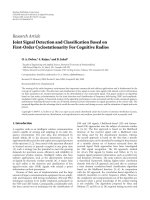
Figure 11: Illustration of how to evaluate the effect of a grid detector on a blockiness metric: an image patch showing visible blocking artifacts
was upscaled with a scaling factor 4/3
×7/3, and the metrics NPBM, GBIM, and LABM were applied to assess the blocking annoyance of the
scaled image.
Table 1: Performance comparison of three blockiness metrics.
Metric Pearson linear correlation Spearman rank-order correlation Outlier tatio
GBIM 0.790 0.912 0.099
LABM 0.834 0.832 0.009
NPBM 0.918 0.924 0
images in the LIVE database. LABM adopts a more flexible
HVS model, that is, the JND profile with a more efficient
integration of luminance and texture masking. As a conse-

quence, the estimation of artifact visibility is more accurate
for LABM than for GBIM. Additionally, LABM is based on a
local estimation of blockiness, in which the distortion and its
visibility due to masking are measured for each individual
coding block of an image. This locally adaptive algorithm
is potentially more accurate in the production of an overall
blockiness score. In comparison with GBIM and LABM, our
metric NPBM shows the highest prediction ability. This is
primarily achieved by the combination of a refined local
metric and a more efficient model of visual masking, both
considering the specific structure of the artifact itself.
4. Evaluation of Specific Metric Components
The blocking annoyance metric, proposed in this paper,
is primarily based on three aspects: (1) a grid detector to
ensure the subsequent local processing; (2) a local distortion
measure; (3) an HVS model for local visibility. To validate
the added value of these aspects, additional experiments were
conducted and a comprehensive comparison to alternatives
is reported. This includes a comparison of
(i) metrics with and without a grid detector;
(ii) the local versus global approach;
(iii) metrics with and without an HVS model;
(iv) different HVS models.
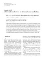
4.1. Metrics with and without a Grid Detector. Our metric
includes a grid detection algorithm to determine the exact
location of the blocking artifacts, and thus to ensure the
calculation of the metric at the appropriate pixel positions.
It avoids the risk of estimating blockiness at wrong pixel
positions, for example, in scaled images. To illustrate the
problem of blockiness estimation in scaled images, a small

experiment was conducted. As illustrated in Figure 11,an
image patch of 64
× 64 pixels was extracted from a low
bit-rate (0.34 bpp) JPEG image of the LIVE database. This
image patch had a grid of blocks of 8
× 8 pixels starting at
its top-left corner, and it clearly exhibited visible blocking
artifacts. It was scaled up with a factor 4/3
× 7/3, resulting
in an image with an effective block size of 11
× 19 pixels.
Blocking annoyance in this scaled image was estimated with
three metrics, that is, NPBM, GBIM, and LABM. Due to the
presence of a grid detector, the NPBM yielded a reasonable
score of 2.2 (NPBM scores range from 0 (no blockiness) to 10
for the highest blocking annoyance). However, in the absence
of a grid detector, both GBIM and LABM did not detect
any substantial blockiness; they had a score of GBIM
= 0.44
and LABM
= 0.67, which corresponds to “no blockiness”
according to their scoring scale (see, [15, 16]). Thus, GBIM
and LABM fail in predicting blocking annoyance of scaled
images, mainly due to the absence of a grid detector. Clearly,
these metrics could benefit in a similar way as our own metric
from including the location of the grid.
Various alternative grid detectors are available in liter-
ature. They all rely on the gradient image to detect the
blocking grid. To do so, they either calculate the FFT for each
single row and column of an image [13] or they calculate

the normalized gradient for every pixel in its two dimensions
[9]. Especially, for large images (e.g., in the case of HD-TV),
these operations are computationally expensive. The main
advantage of our proposed grid detector lies in its simplicity,
EURASIP Journal on Advances in Signal Processing 11
Metric
GBIM
LABM
NPBM
MUR
2.5
2
1.5
1
0.5
0
Figure 12: Comparison of the computational cost of three metrics,
using model utilization ratio (MUR).
compared to existing alternatives in literature. Such as in
the approach reported in [18], we first project the gradient
image into a 1-D signal and then enhance the signal maxima
using once a median filter. In addition, the size and offset
of the grid are extracted from the resulting 1-D signal using
a DFT. The latter is less computationally expensive than
the approach chosen in [18], being a complex maximum-
likelihood method.
Apart from affecting the blocking grid position, scaling
may also affect the blocking artifact visibility [9]. This aspect,
however, is not yet taken into account in our proposed
metric.

4.2. Local versus Global Approach. The difference in local
versus global approach can be best understood by comparing
their basic formulation. A local metric, as proposed in this
paper, is based on a general formulation of the form MF1:
MF1
=
1
n
n

k=1
[LPB(k) × M(k)], (17)
where k denotes the pixel location of blocking artifacts, and
LPB and M denote the local pixel-based blockiness (see (7))
and the HVS model embedded, respectively. Both of them
are calculated locally within a region of the image centered
on individual blocking artifacts.
A global metric as, for example, used in GBIM [15]is
based on a general formulation of the form MF2:
MF2
=


G(i, j)
block-edge
×M(i, j)
block-edge





G(i, j)
non-block-edge
×M(i, j)
non-block-edge


, (18)
where G denotes the interpixel difference (see (1)), M
denotes the HVS model embedded, and
·is the L2-
norm. The numerator is calculated at the location of blocking
artifacts, while the denominator is calculated for pixels which
are not on the blocking grid.
An obvious advantage of the local approach over the
global approach is already revealed by their formulation:
MF1 only calculates the HVS model for pixels on the
blocking grid, while MF2 needs to calculate the HVS model
for all pixels in the image. Since the major cost of an HVS-
based blockiness metric is usually introduced by the human
vision model, reducing the number of times the HVS model
calculated in the whole process is highly beneficial for the
computational load. The computational cost related to the
number of times the HVS model has to be calculated in a
metric can be quantified by means of a model utilization ratio
(MUR), which is simply defined as the total number of times
T
M
that the HVS model is computed, divided over the total
number of pixels M

×N in the image
MUR
=
T
M
M ×N
. (19)
Evidently, the lower this ratio, the simpler the metric is.
Figure 12 shows the MUR for GBIM, LABM, and NPBM,
respectively. Both GBIM and LABM calculate the human
vision model for every pixel in an image, which yields a
MURof1.ForGBIMtheMURisincreasedbyafactorof
2, since masking is estimated for the horizontal and vertical
blockiness directions separately. For our metric the MUR is
only 0.25 in case of a block size of 8
×8 pixels, which is a direct
result of calculating the HVS model only at detected blocking
artifacts. This implies that when neglecting the difference in
computational cost between the various HVS models for a
moment, the computational load of NPBM is reduced by
approximately 7/8 with respect to GBIM and by 3/4 with
respect to LABM.
Of course, in this respect also the complexity of the HVS
model used needs to be taken into account. This is further
discussed in Section 4.4, taking into account various HVS
models. Additionally, there also is a performance difference
between the local and global approaches. But, since the
performance gain depends on the specific choice of HVS
used, this point is also discussed in Section 4.4.
4.3. Metrics with and without an HVS Model. To validate

the added value of including an HVS model in a blockiness
metric, we compared our proposed HVS-based metric
NPBM to the state-of-the-art non-HVS-based metric of [9],
whichisreferredtoasNBAM.NBAMisalsoaglobalmetric
formulated according to (18), but instead of using an HVS
model, it replaces the interpixel difference by the relative
gradient in order to determine the visual strength of a block
discontinuity. It was achieved a promising performance
over the entire LIVE database as indicated by the Pearson
correlation coefficient (after nonlinear regression) of 0.92,
which is comparable to our metric with a Pearson correlation
coefficient of 0.94. However, because of the absence of
an HVS model, the robustness of NBAM against image
content might be an issue. It may be doubted to what extent
the objective metric is able to predict blockiness in more
demanding images, for example, for a set of highly textured
images, compressed at very low bit-rates, for which visual
masking is important.
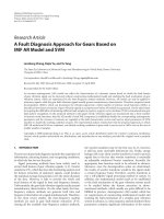
To evaluate this, a subset of six highlytextured images,
as shown in Figure 13, was selected from the twentynine
source images of the LIVE database. Including different
compression levels, this resulted in a test database of 50
12 EURASIP Journal on Advances in Signal Processing
Highly textured source images
NBAM
(without HVS)
NBAM
(with HVS)
50 JPEG images
(LIVE)

Correlation
(Pearson)
0.74
Correlation
(Pearson)
0.94
MOS
0
1
2
3
4
5
6
7
8
9
10
11
NBAM
01234567891011
MOS
0
1
2
3
4
5
6
7

8
9
10
11
NBAM
01234567891011
Figure 13: Illustration of the added value of including an HVS model in a blockiness metric: a database of 50 highly textured JPEG images
was extracted from the LIVE database, and blockiness annoyance was estimated with the metrics NBAM (without HVS) and NPBM (with
HVS). The prediction performance is given in terms of the Pearson correlation coefficient.
Local metric
formulation MF1
NPBM
MF1(M
= VC)
LM
JND
MF1(M = JND)
LM
WF
MF1(M = WF)
LM
NO
MF1(M = 1)
LIVE
(233 JPEG images)
Correlation (Pearson)
0.92
Correlation (Pearson)
0.87
Correlation (Pearson)

0.87
Correlation (Pearson)
0.87
Figure 14: Illustration of the comparison of various HVS models: a blockiness metric (i.e., MF1) having four optional HVS models
embedded is tested with the LIVE database, and the performance for each resulting metric is quantified by the Pearson correlation coefficient.
JPEG images with their corresponding MOS scores extracted
from the LIVE database. For these images, texture masking
was dominant, that is, most blocking artifacts were largely
masked by background nonuniformity.
The blockiness metrics, NPBM and NBAM, were applied
to this test database. Their prediction performance is quanti-
fied by the Pearson correlation coefficient (without nonlinear
regression) as illustrated in Figure 13. As expected, the simple
metric NBAM fails in accurately predicting the subjective
ratings of this subset of demanding images, mainly due to
the lack of an HVS model. NPBM shows a robust prediction
ability, resulting in a high correlation with the subjective
MOS.
4.4. Comparison of Different HVS Models. To c o m p a r e
the added value of our proposed HVS model to existing
alternatives, various HVS models M have been embedded in
the general formulation of our local metric (see MF1 (17)).
For M we used four alternatives:
(i) VC model (i.e., our proposed HVS model);
(ii) JND model (i.e., the JND profile model based on
[21]);
(iii) WF model (i.e., the HVS model used in GBIM [15]);
(iv) M
= 1 model (i.e., no HVS model embedded).
Doing so, resulted in four blockiness metrics, which we

refer to as LM
VC
(i.e., NPBM), LM
JND
,LM
WF
,andLM
NO
,
respectively. These four metrics were applied to the LIVE
database of 233 JPEG images. The metric performance was
quantified by the Pearson correlation coefficient (without
nonlinear regression) as illustrated in Figure 14.Insuch
a scenario, the performance difference between any two
metrics can be attributed to the HVS model embedded.
LM
NO
(i.e., MF1 without any HVS model) is used as the
benchmark, and the HVS model gain is determined by
calculating the difference in Pearson correlation coefficient
between the metric LM
NO
and any of the other three metrics.
Figure 14 clearly illustrates that our HVS model yields
the biggest gain compared to the other three alternatives. For
the local approach defined as MF1 in (17), there is no added
value of using the JND or WF model in the metric, since their
performance is comparable to that of the metric without
HVS model. This may, of course, be due to the fact that
the JND and WF models were not designed to be combined

with our proposed local metric. Our VC model, on the other
hand, is designed together with the definition of MF1, and as
EURASIP Journal on Advances in Signal Processing 13
Global metric
formulation MF2
GM
VC
MF2(M = VC)
GM
JND
MF2(M = JND)
GBIM
MF2(M
= WF)
GM
NO
MF2(M = 1)
LIVE
(233 JPEG images)
Correlation (Pearson)
0.86
Correlation (Pearson)
0.80
Correlation (Pearson)
0.79
Correlation (Pearson)
0.78
Figure 15: Illustration of the comparison of various HVS models: a blockiness metric (i.e., MF2) having four optional HVS models
embedded is tested with the LIVE database, and the performance for each resulting metric is quantified by the Pearson correlation coefficient.
Pearson correlation coefficient

M
= NO M = WF M = JND M = VC
M-HVS model embedded
0.95
0.9
0.85
0.8
0.75
0.7
Local metric (MF1)
Global metric (MF2)
Figure 16: Comparison of the local and global approaches to
a blockiness metric, and of metrics with different HVS models
embedded.
aresultahighcorrelationcoefficient is found for the NPBM
metric.
To investigate whether our HVS model is also valuable for
traditionally used global metrics (see MF2 in (18)), the same
experiment was repeated by substituting in MF2 the four
options for M. This yielded another set of four blockiness
metrics, which are referred to as GM
VC
,GM
JND
,GM
WF
(i.e.,
GBIM), and GM
NO
, respectively. Their performance when

applied to the LIVE database is illustrated in Figure 15.
It illustrates that also for a global metric our HVS model
has the largest added value. In this case, however, also the WF
and JND models have some added value. It should be noted,
however, that in our evaluations the WF and JND models
were implemented as described in the original publications
(i.e., [15, 21]). Some parameters in the implementations may
be adjusted specifically to the LIVE database to provide a
better correlation.
To summarize, the contribution of our proposed HVS
model to a blockiness metric is consistently shown, inde-
pendent of the specific design of the blockiness metric. In
addition, a number of significant simplifications used in
our HVS model are already discussed in Section 2.3.The
complexity of our VC model is comparable to that of the
WF model, both of them use a simple weighting function for
local visibility. However, the JND model is a rather complex
HVS model, mainly due to the difficulties in estimating
the visibility thresholds for various masking effects and in
combing different JND thresholds. The simplicity of the
VC model itself, coupled with its specific design for a
local approach to avoid calculating it on irrelevant pixels,
consequently makes this HVS model especially promising in
terms of real-time applications.
An additional interesting finding from the comparison of
Figures 14 and 15 is that there is indeed a gain in performance
applying the MF1 formulation (local approach) instead of
the MF2 formulation (global approach), independent of the
HVS model used. In the absence of any HVS model, the gain
of MF1 over MF2 (i.e., from LM

NO
to GM
NO
) corresponds to
an increase in the Pearson correlation coefficient from 0.78 to
0.87. For the other HVS models, the corresponding numbers
are summarized in Figure 16. It confirms that a promising
performance is achieved when applying the local approach in
a blockiness metric.
5. Conclusions
In this paper, a novel blockiness metric to assess blocking
annoyance in block-based DCT coding is proposed. It is
based on the following features.
(i) A simple grid detector to ensure the effectiveness of
the blockiness metric and to account for deviations
in the blocking grid of the incoming signal or as a
consequence of spatial scaling.
(ii) A local pixel-based blockiness value that measures the
strength of the distortion within a region of the image
centered around each individual blocking artifact.
(iii) A simplified and more efficient model of visual mask-
ing, exhibiting an improved robustness in terms of
content independency, and allowing suprathreshold
estimation of perceived annoyance.
14 EURASIP Journal on Advances in Signal Processing
An advantage of the proposed approach, especially in
case of real-time application, is that the additional com-
putational cost introduced by the HVS is largely reduced
by eliminating calculations of the human vision model for
nonrelevant pixels. This is primarily accomplished taking

advantage of the locality of both the pixel-based blockiness
value and the visibility model. Nonetheless, the metric is
mainly used to assess overall blockiness annoyance, which
is simply done by summing the local contributions over the
whole image.
Experimental results show that our proposed blockiness
metric results in a strong correlation with subjective data and
outperforms state-of-the-art metrics in terms of prediction
accuracy. Combined with its practical reliability and compu-
tational efficiency, our metric is a good alternative for real-
time implementation.
References
[1] Z. Wang and A. C. Bovik, Modern Image Quality Assessment,
Synthesis Lectures on Image, Video, & Multimedia Processing,
Morgan & Claypool, San Rafael, Calif, USA, 2006.
[2]C.C.Koh,S.K.Mitra,J.M.Foley,andI.E.J.Heynderickx,
“Annoyance of individual artifacts in MPEG-2 compressed
video and their relation to overall annoyance,” in Human
Vision and Electronic Imaging X, vol. 5666 of Pro ceedings of
SPIE, pp. 595–606, San Jose, Calif, USA, January 2005.
[3] S. Winkler, “Issues in vision modeling for perceptual video
quality assessment,” Sig nal Processing, vol. 78, no. 2, pp. 231–
252, 1999.
[4] Z. Yu and H. R. Wu, “Human visual system based objective
digital video quality metrics,” in Proceedings of the 5th Interna-
tional Conference on Sig nal Processing (WCCC-ICSP ’00), vol.
2, pp. 1088–1095, Beijing, China, August 2000.
[5] Z. Yu, H. R. Wu, S. Winkler, and T. Chen, “Vision-model-
based impairment metric to evaluate blocking artifacts in
digital video,” Proceedings of the IEEE, vol. 90, no. 1, pp. 154–

169, 2002.
[6] E.M.Yeh,A.C.Kokaram,andN.G.Kingsburg,“Perceptual
distortion measure for edgelike artifacts in image sequences,”
in Human Vision and Electronic Imaging III, vol. 3299 of
Proceedings of SPIE, pp. 160–172, San Jose, CA, USA, January
1998.
[7] S. A. Karunasekera and N. G. Kingsbury, “Distortion measure
for blocking artifacts in images based on human visual
sensitivity,” IEEE Transactions on Image Processing, vol. 4, no.
6, pp. 713–724, 1995.
[8] M. Yuen and H. R. Wu, “A survey of hybrid MC/DPCM/DCT
video coding distortions,” Signal Processing,vol.70,no.3,pp.
247–278, 1998.
[9] R. Muijs and I. Kirenko, “A no-reference blocking artifact
measure for adaptive video processing,” in Proceedings of the
13th European Signal Processing Conference (EUSIPCO ’05),
Antalya, Turkey, September 2005.
[10] I. O. Kirenko, R. Muijs, and L. Shao, “Coding artifact reduc-
tion using non-reference block grid visibility measure,” in
Proceedings of the IEEE International Conference on Multimedia
and Expo (ICME ’06), pp. 469–472, Toronto, Canada, July
2006.
[11] Z. Wang, H. R. Sheikh, and A. C. Bovik, “No reference
perceptual quality assessment of JPEG compressed images,”
in Proceedings of the IEEE International Conference on Image
Processing (ICIP ’02), vol. 1, pp. 477–480, Rochester, NY, USA,
September 2002.
[12] R. V. Babu, S. Suresh, and A. Perkis, “No-reference JPEG-
image quality assessment using GAP-RBF,” Signal Processing,
vol. 87, no. 6, pp. 1493–1503, 2007.

[13] Z. Wang, A. C. Bovik, and B. L. Evans, “Blind measurement
of blocking artifacts in images,” in Proceedings of the IEEE
International Conference on Image Processing (ICIP ’00), vol.
3, pp. 981–984, Vancouver, Canada, September 2000.
[14] S. Liu and A. C. Bovik, “Efficient DCT-domain blind measure-
ment and reduction of blocking artifacts,” IEEE Transactions
on Circuits and Systems for Video Technology, vol. 12, no. 12,
pp. 1139–1149, 2002.
[15] H. R. Wu and M. Yuen, “A generalized block-edge impairment
metric for video coding,” IEEE Signal Processing Letters, vol. 4,
no. 11, pp. 317–320, 1997.
[16] F. Pan, X. Lin, S. Rahardja, et al., “A locally adaptive algorithm
for measuring blocking artifacts in images and videos,” Signal
Processing: Image Communication, vol. 19, no. 6, pp. 499–506,
2004.
[17] E. Lesellier and J. Jung, “Robust wavelet-based arbitrary grid
detection for MPEG,” in Proceedings of the IEEE International
Conference on Image Processing (ICIP ’02)
, vol. 3, pp. 417–420,
Rochester, NY, USA, September 2002.
[18] S. Tjoa, W. S. Lin, H. V. Zhao, and K. J. R. Liu, “Block
size forensic analysis in digital images,” in Proceedings of
the IEEE International Conference on Acoustics, Speech, and
Signal Processing (ICASSP ’07), vol. 1, pp. 633–636, Honolulu,
Hawaii, USA, April 2007.
[19] H. Liu and I. Heynderickx, “A no-reference perceptual block-
iness metric,” in Proceedings of the IEEE International Confer-
ence on Acoustics, Speech, and Signal Processing (ICASSP ’08),
pp. 865–868, Las Vegas, Nev, USA, March-April 2008.
[20] T. N. Pappas and R. J. Safranek, “Perceptual criteria for

image quality evaluation,” in Handbook of Image and Video
Processing, pp. 669–684, Academic Press, New York, NY, USA,
2000.
[21] C H. Chou and Y C. Li, “A perceptually tuned subband
image coder based on the measure of just-noticeable-
distortion profile,” IEEE Transactions on Circuits and Systems
for Video Technology, vol. 5, no. 6, pp. 467–476, 1995.
[22] S. Winkler, Vision models and quality met rics for image
processing applications, Ph.D. dissertation, Department of
Electrical Engineering, EPFL, Lausanne, Switzerland, 2002.
[23] K. I. Laws, “Texture energy measures,” in Proceedings of
the DARPA Image Understanding Workshop, pp. 47–51, Los
Angeles, Calif, USA, November 1979.
[24] B. Girod, “The information theoretical significance of spatial
and temporal masking in video signals,” in Human Vision,
Visual Processing, and Digital Display, vol. 1077 of Proceedings
of SPIE, pp. 178–187, Los Angeles, Calif, USA, January 1989.
[25] X. Yang, W. Lin, Z. Lu, E. Ong, and S. Yao, “Motion-
compensated residue preprocessing in video coding based
on just-noticeable-distortion profile,” IEEE Transactions on
Circuits and Systems for Video Technology,vol.15,no.6,pp.
742–751, 2005.
[26] H. R. Sheikh, Z. Wang, L. Cormack, and A. C. Bovik, “LIVE
image quality assessment database Release 2,” March 2008,
/>[27] VQEG, “Final report from the video quality experts group
on the validation of objective models of video quality
assessment,” Tech. Rep., Video Quality Experts Group, Ottawa,
Canada, August 2003, />