Báo cáo hóa học: " Research Article A Common Coordinates/Heading Direction Generation Method for a Robot Swarm with Only RSSI-Based Ranging" ppt

Hindawi Publishing Corporation
EURASIP Journal on Advances in Signal Processing
Volume 2009, Article ID 434597, 11 pages
doi:10.1155/2009/434597
Research Article
A Common Coordinates/Heading Direction Generation Method
for a Robot Swarm with Only RSSI-Based Ranging
Shinsuke Hara, Tatsuya Ishimoto, Masaya Kitano, and Tetsuo Tsujioka
Graduate School of Engineering, Osaka City University, Sumiyoshi-ku, Osaka 558-8585, Japan
Correspondence should be addressed to Shinsuke Hara,
Received 31 July 2008; Revised 30 December 2008; Accepted 18 February 2009
Recommended by Frank Ehlers
In the motion control of a microrobot swarm, a key issue is how to autonomously generate a set of common coordinates among
all robots and how to notify each robot of its heading direction in the generated common coordinates without any special devices
for estimating location and bearing. This paper proposes a set of common coordinates and a heading direction generation method
for a robot swarm with only received signal strength indicator (RSSI) measured through wireless communications. We explain the
principle of the proposed method and show some computer simulation results on the location and direction estimation errors.
Finally, we demonstrate some experimental results using a swarm composed of five robots with the IEEE 802.15.4 standard as its
wireless communication tool.
Copyright © 2009 Shinsuke Hara et al. This is an open access article distributed under the Creative Commons Attribution License,
which permits unrestricted use, distribution, and reproduction in any medium, provided the original work is properly cited.
1. Introduction
A group of wirelessly networked robots is called a “robot
swarm” [1, 2], and its promising applications include smart
pills, drug delivery systems, and rescue systems. When a
robot swarm is put into a new environment, member robots
first start communicating with other (members) robots by
wireless communication tool to recognize members of the
swarm. Next, they try to understand their situations in
the new environment by wireless communication, sharing
and analyzing information obtained through their sensors.

Finally, they decide and make a motion also by wireless com-
munication to accomplish a given unified task as a group.
Therefore, wireless communications play an important role
in information transmission and motion control of robot
swarm [3].
Especially for a microrobot swarm, since the size, energy,
and memory of each robot are severely limited, functions of
the swarm should be distributed over all robots; some robots
are equipped with only the function of delivering energy to
other robots, others are occupied with sensing the outside
world and so on. The common function that all robots can
have is wireless communications, so the functions imbed-
dable in wireless communications should be supported by
the wireless communications. For example, ranging, namely,
measuring the distance between a transmitter and a receiver,
is easily supportable in wireless communications, so it should
be supported by wireless communication protocol, without
any special devices such as global positioning system (GPS)
and geomagnetic sensors, which can be used to determine
location and bearing.
Now, almost all of wireless communication standards,
such as the IEEE 802.11 and 802.15.4 [4], support the
function of measuring received signal power called “received
signal strength indicator (RSSI).” This is because the RSSI can
be measured by a very simple electronic circuit and its use for
estimating wireless link quality effectively works. The RSSI
drastically changes due to fading, shadowing, and near/far
effect in wireless communications among robots because a
signal emitted from a robot is reflected and shadowed by
other robots [5]. However, once the medium of channel,

types of transmitter/receiver antennas, type of carrier wave,
and frequency/bandwidth of the carrier are given, we can
derive the statistical model on the channel variation, namely,
the relationship between the RSSI and distance, so a receiver
can range for a transmitter with the RSSI. The advantage
of RSSI ranging is that it is independent of the types of
waveforms and that it is workable even in non-line-of-sight
(NLOS) condition, although its accuracy is low. Therefore,
in this paper, we assume an RSSI-based ranging with a
2 EURASIP Journal on Advances in Signal Processing
prior knowledge on the relationship between the RSSI and
distance.
There are mainly two methods of motion control for
robot swarms, such as by ranging [6] and by localization
[7]. The ranging-based motion control means that a leader
robot decides and makes a motion, and other robots
just follow it keeping the distance to it constant without
knowing their locations and heading directions. On the other
hand, the localization-based motion control means that all
robots make their motions knowing their locations and
heading directions in a set of common coordinates. In the
localization-based motion control for a microrobot swarm,
how to autonomously generate a set of common coordinates
among robots and how to notify each robot of its heading
direction in the coordinates without any special devices are
key issues.
There have been many papers related to multirobot
systems in the research fields of robotics and wireless
communications. For the purpose of multirobot exploration
and collaboration [8], several self-localization techniques

have been proposed. For example, the tradeoff between
localization efficiency and accuracy is discussed [9], and a
Markov-based technique is proposed [10]. In these applica-
tions, to precisely control multirobots, intelligent devices are
used, such as sonar, laser ranger finder, image sensor, and
camera [11]. On the other hand, for mobile sensor networks,
localization techniques without such intelligent devices are
proposed [12, 13]. However, in these applications, GPS is
often assumed for obtaining the locations of communication
nodes, and the propagation characteristic of wireless signal is
ignored.
In this paper, we propose a set of common coordinates
and a heading direction generation method for a robot
swarm with only RSSI-based ranging. Our key idea is based
on the fact that when a robot receives a packet from another
robot, it newly measures its RSSI related to the distance
between them so the robot can improve its accuracy. In a fully
networked robot swarm, our distributed localization method
makes use of the effect, which has never been discussed in
other literatures, so it can iteratively improve the location
accuracy of each robot during their packet exchanging
process. This accurate localization results in generating a
set of accurate common coordinates thus accurate heading
directions among robots.
In the research on swarm robotics, demonstration of
the performance by experiments is important. Therefore,
with commercially available wireless communication devices
based on the IEEE 802.15.4 standard, we developed a swarm
composed of 5 robots and conducted some experiments
in indoor and outdoor environments. Here, to derive

the localization algorithm, we took into consideration the
propagation characteristic of the IEEE 802.15.4 signal. This
algorithm is based on maximum likelihood estimation,
which gives unbiased estimator [14].
The paper is organized as follows. Section 2 states the
problem of common coordinates and heading direction
generation and some assumptions to solve the problem.
Section 3 presents the details of the proposed method, which
is composed of three major components. Section 4 shows
Individual
heading direction
All robots are networked
wirelessly
Robot
(a) Initial stage
Common
heading
direction
Common
coordinates
y
x
0
(b) Common coordinates/heading direction genera-
tion
Figure 1: Problem of common coordinates/heading direction
generation.
some computer simulation results on the performance of
the proposed method in terms of the location and direction
estimation errors. Section 5 shows the experimental results

using the swarm. Finally, Section 6 concludes the paper.
2. Problem Statement of
Common Coordinates/Heading
Direction Generation
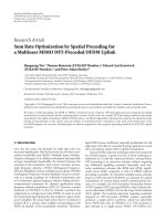
Figure 1 shows the problem of the common coordinates and
heading direction generation discussed in the paper.
In the initial stage, it is assumed that all robots have been
wirelessly networked with each other, but that each robot
has its own (different) individual heading direction (e.g.,
north) and no knowledge of its coordinates. The problem
is generating a set of common coordinates among all of the
robots and notifying each robot of its heading direction in
the generated coordinates using only a ranging capability in
wireless communications. Here, for the sake of simplicity,
we assume that all of the robots are on the same plane,
namely, we discuss a two-dimensional common coordinate
generation: (x, y). Note that the proposed method can be
easily extended to the three-dimensional case.
A signal emitted from a robot experiences multipath
reflections by other robots and surrounding obstacles, and
furthermore, other robots in motion introduce a time-
varying aspect to the signal received by each robot [5].
Therefore, the power (RSSI) of a received signal fluctuates in
time. For the IEEE 802.15.4 signal, which has been adopted
EURASIP Journal on Advances in Signal Processing 3
in our experiment, we can assume the following two-layered
model on the distribution of the received power: [15, 16]
P = αd
−β
,(1)

p(P
| d) =
1
P
exp

−
P
P

,(2)
where P,
P,andd denote the received power, the average
received power, and the distance between a transmitter robot
and a receiver robot, respectively, and p(P
| d)denotes
the conditional probability density function (pdf )ofP
when d is given. In (1), α and β are the constants that are
uniquely determined by the medium of the channel and the
carrier frequency and bandwidth of the signal. Note that
the prerequisite knowledge on the channel parameters is not
necessarily required, namely, they can be jointly estimated
with the locations of robots [17].
3. Proposed Common Coordinates/Heading
Direction Generation Method
The proposed common coordinates/heading direction gen-
eration method is composed of three elements, such as pivot
robots selection, location estimation, and heading direction
estimation.
3.1. Pivot Robots Selection. On a plane, if we know the loca-

tions of three different robots, we can uniquely determine the
location of any robot according to these three locations. The
proposed pivot robots selection chooses three robots with
different locations as “pivot robots.” Here, we assume that
there are M robots communicating with each other, and the
robots are autonomously numbered at random as 1 to M (ID
number).
In the first step, each robot broadcasts N
o
“hello packets”
containing its ID number to all other robots. Defining P
ijs
as
the RSSI of the sth packet (s
= 1, , N
o
)transmittedfrom
the ith robot and received at the jth robot, with (1), the jth
robot can calculate the average RSSI and then the distance
between them as (j
= 1, ,N
o
, i
/
= j)
P
ij
=
1
N

o
N
o

s=1
P
ijs
,
(3)
d
ij
=

P
ij
α

−1/β
,
(4)
and broadcasts d
ij
to all other robots. In this way, all of the
robots can share the information on the distances between
all pairs of robots d
ij
(i, j = 1, , M, i
/
= j).
In the second step, each robot autonomously selects a

pair of robots separated by the largest distance:
select robots i and j,
i, j
= arg
i,j
max

d
ij
| i, j = 1, , M, i
/
= j

,
(5)
and each arbitrarily designates one of the two robots as
the “master pivot robot”, with the location vector of Z
1
=
#1
#3
d
13
d
14
d
34
#4
d
23

d
24
d
12
#2
Z
2
= [d
12
,0]
Z
1
= [0,0]
Z
3
= [X
3
, Y
3
> 0]
Figure 2: Pivot robots selection with M = 4.
[X
1
, Y
1
] = [0, 0], whereas the other robot is designated as
the “slave pivot robot”, with the location of Z
2
= [X
2

, Y
2
] =
[d
ij
(> 0), 0].
In the third step, as “another slave pivot robot,” each
robot autonomously selects a robot located farthest from the
pivot robots selected in the second step:
select robot k,
k
= arg
k
max

d
ik
+ d
kj
| k = 1, , M, k
/
=i, j

,
(6)
with the location vector of Z
3
= [X
3
, Y

3
> 0] satisfying
X
2
3
+ Y
2
3
= d
2
ik
,

d
ij
−X
3

2
+ Y
2
3
= d
2
kj
.
(7)
In this way, each robot autonomously selects three pivot
robots that are located far from each other. Finally, each
robot then renumbers the master pivot robot as 1. The slave

pivot robots are renumbered as 2 and 3, and the other
nonpivot robots are renumbered as 4 to M. Figure 2 shows
an example of the (far) pivot robots selection with M
= 4
after the renumbering is finished.
Note that robots can randomly select three robots as one
alternative and also they can select three robots located in
close proximity to each other as another alternative. We will
compare the location estimation performance among the far,
random, and near pivot robots selections in Section 4.
3.2. Iterative Maximum Likelihood Location Estimation.
Once the three pivot robots have been selected, they begin to
broadcast their locations to all other robots. Here, we apply
the index l to the pivot robots (l
= 1, 2,3), whereas the index
m is applied to the nonpivot robots (m
= 4, ,M).
In the first step, each pivot robot broadcasts N packets
containing its ID number and location to all other robots.
Defining the location vector of the mth nonpivot robot as
z
m
= [x
m
, y
m
]; the distance between the lth pivot robot and
the mth nonpivot robot is written as
d
lm

=


Z
l
−z
m


=


X
l
−x
m

2
+

Y
l
− y
m

2
.
(8)
4 EURASIP Journal on Advances in Signal Processing
Pivot #1

Pivot #3
Pivot #2
P
241
#4
#5
P
141
P
341
(a) First step for nonpivot robot #4
Pivot #1
Pivot #3
Pivot #2
P
251
#4
#5
P
151
P
351
(b) First step for nonpivot robot #5
Pivot #1
Pivot #3
Pivot #2
P
242
#4
#5

P
142
P
342
P
541
(c) Second step for nonpivot robot #4
Pivot #1
Pivot #3
Pivot #2
P
252
#4
#5
P
152
P
352
P
451
(d) Second step for nonpivot robot #5
Figure 3: Iterative maximum likelihood location estimation with M = 5, N = 1, and Q = 1.
Then, define the RSSI vector as
P
mn
=

P
1mn
, P

2mn
, P
3mn

,(9)
where P
lmn
denotes the RSSI of the nth packet (n = 1, , N)
transmitted from the lth pivot robot and received at the mth
nonpivot robot. Since the unknown location of the nonpivot
robot z
m
is estimated with the measured RSSIs, the log-
likelihood function on z
m
is written with the conditional pdf
of P
mn
(n = 1, , N) when z
m
is given as
L

z
m

=
log p

P

m1
, P
m2
, ,P
mN
| z
m

. (10)
Assuming that P
lmn
is statistically uncorrelated with P
lmn

(n
/
=n

)(temporal whiteness)andP
l

mn
(l
/
=l

)(geographical
whiteness), replacing d by d
lm
and P by P

lmn
,respectively,in
(1)and(2), (10) yields
L

z
m

=
log
⎡
⎣
N

n=1
3

l=1

1
αd
lm
−β
exp

−
P
lmn
αd
lm

−β

⎤
⎦
=
N
3

l=1

log

1
αd
lm
−β

−

N
n=1
P
lmn
/N
αd
lm
−β

.
(11)

The ML estimation gives
z
m0
= [x
m0
, y
m0
], which maximizes
(11)[14]
∂L

z
m

∂z
m





z
m0
=[x
m0
,y
m0
]
= 0(m = 4, , M). (12)
Since the locations of the nonpivot robots have been

estimated in the first step, the robots also begin to broadcast
their ID numbers and estimate locations to all other robots.
In the second step, each nonpivot robot estimates its location
each time it receives broadcast packets from all other robots,
and then broadcasts back a packet containing its newly
estimated location with its ID number to all other robots.
On the other hand, each pivot robot improves its location
accuracy every time it receives broadcast packets from other
pivot robots.
Define the estimated location vectors of the lth pivot
robot and the mth nonpivot robot with the qth broadcast
packet as Z
lq
and z
mq
(q = 1, ,Q), respectively. Z
lq
can be
estimated by the same procedure in the pivot robots selection
replacing N
o
by q in (3). Here, the distance between the
lth pivot robot and the mth nonpivot robot with the qth
broadcast packet is written as
d
lmq
=


Z

lq
−z
mq


. (13)
On the other hand, when the mth nonpivot robot receives
the qth broadcast packet from the m

th nonpivot robot with
the RSSI of P

m

mq
, which contains the estimated location
vector of the m

th nonpivot robot z
m

(q−1)
, it can use the
m

th nonpivot robot as a pivot robot with the location vector
of
z
m


(q−1)
(m

= 4, , M, m

/
=m). Namely, the distance
between the mth nonpivot robot and the m

th nonpivot
robot with the temporarily known location vector of
z
m

(q−1)
is
d
m

mq
=


z
m

(q−1)
−z
mq



=



x
m

(q−1)
−x
mq

2
+


y
m

(q−1)
− y
mq

2
,
(14)
EURASIP Journal on Advances in Signal Processing 5
so the log-likelihood function on z
mq
is written as

L

z
mq

=
log
⎡
⎣
q

q

=1
3

l=1
⎧
⎨
⎩
1
αd
lmq

−β
exp
⎛
⎝
−
P

lmq

+N
αd
lmq

−β
⎞
⎠
⎫
⎬
⎭
·
M

m

=4
m

/
=m
⎧
⎨
⎩
1
αd
m

mq


−β
exp
⎛
⎝
−
P

m

mq

αd
m

mq

−β
⎞
⎠
⎫
⎬
⎭
⎤
⎥
⎥
⎥
⎦
=
q


q

=1
⎡
⎣
3

l=1
⎧
⎨
⎩
log
⎛
⎝
1
αd
lmq

−β
⎞
⎠
−
P
lmq

+N
αd
lmq


−β
⎫
⎬
⎭
+
M

m

=4
m

/
=m
⎧
⎨
⎩
log
⎛
⎝
1
αd
m

mq

−β
⎞
⎠
−

P
m

mq

αd
m

mq

−β
⎫
⎬
⎭
⎤
⎥
⎥
⎥
⎦
.
(15)
The ML estimation yields z
mq
= [x
mq
, y
mq
], which maxi-
mizes (11)
∂L


z
mq

∂z
mq





z
mq
=[x
mq
,y
mq
]
= 0(m = 4, ,M). (16)
In this way, each nonpivot robot and each slave pivot
robot can iteratively estimate their current locations with the
previous locations of the other pivot robots and nonpivot
robots up to q
= Q. Figure 3 shows an example of iterative
maximum likelihood location estimation with M
= 5, N =
1, and Q = 1.
Note that all robots autonomously generate a set of
common coordinates, so the coordinates have ambiguities
such as translation, rotation, and negation with respect to

the coordinates of an observer (operator) of the wirelessly
networked robots. However, this is not critical because we
can determine the relationship between the two coordinates.
3.3. Heading Direction Estimation. After the pivot robots
selection and iterative maximum likelihood location estima-
tion, all robots have generated a set of common coordinates,
and each robot knows its location in the generated coordi-
nates.
In the 0th step, the robots autonomously divide the set
of all robots into U subsets with equal numbers of robots.
Next, in the uth location/direction estimation step (u
=
1, ,U)withQ broadcast packets, each robot in the uth
subset moves through a distance of B, according to its own
individual heading direction and stops, and its location is
then estimated, starting with the robots in the other subsets
(u

= 1, ,U, u

/
=u) as pivot robots in the same manner as
the iterative maximum likelihood location estimation. This
process is repeated until u
= U, and then the mth robot
(m
= 1, , M) can determine its location before and after
the movement, namely, z
b
m

= [x
b
m
, y
b
m
]andz
a
m
= [x
a
m
, y
a
m
].
Finally, with the direction of the movement vector, the robot
can estimate the angle between its heading direction and the
x-axis in the generated coordinates, that is,

θ
m
= arg

z
a
m
−z
b
m


. (17)
Figure 4 shows an example of heading direction estima-
tion with M
= 6andU = 2. Note that if a moving robot
collides with another stationary robot, the moving robot
returns to its original location, changes its heading direction
by +γ degrees, and moves again. This process is repeated
until the robot has successfully finished moving through
distance of B without collision.
4. Computer Simulation Results
As shown in Section 5, we have developed a swarm composed
of five robots to demonstrate the proposed common coordi-
nates and heading direction generation method experimen-
tally, where the PHY/MAC protocol is based on the IEEE
802.15.4 standard. Therefore, we determined the values of
the two parameters in (1)asα
= 2.36 × 10
−6
and β = 2.37
by a channel measurement experiment using a set of IEEE
802.15.4-based transceivers in a room.
In a computer simulation, we assume a field of
10 m
× 10 m and randomly select the locations of robots in
the field. To speed up the process of generating the common
coordinates and heading direction, we set N
o
= 1andN = 1.
Furthermore, we refer to the number of broadcast packets

(Q) as the “number of iterations.”
Figure 5 shows the root mean square (RMS) location
estimation error with respect to the number of iterations for
the case of six robots. For all of the robots, as the number of
iterations increases, the location estimation error gradually
decreases because more packets (information) can be used
for location estimation. For the pivot robots, the master
robot is located at the origin, so its location estimation
error is always zero, whereas the location estimation error
of slave robot 3 is affected by that of slave robot 2, so the
location estimation error of slave robot 3 is worse than that
of slave robot 2. On the other hand, for the nonpivot robots,
location estimation errors are affected by the worst location
estimation error among the location estimation errors of the
pivot robots. Therefore, the location estimation errors of the
nonpivot robots are worse than the location estimation error
of slave robot 3. However, there is no significant difference
in the location estimation error among the nonpivot robots.
In the following, the location estimation error is averaged
over all types of robots such as master pivot, slave pivot, and
nonpivot robots.
Figure 6 shows the effect of pivot robots selection for
the case of six robots. The distances between pivot robots
and nonpivot robots should be shorter because they have
larger receiving powers and, consequently, smaller location
estimation errors. In this sense, the case in which nonpivot
robots are located in the area of a triangle formed by pivot
robots as its three vertexes provides better location estima-
tion performance. When three robots at distant locations
from one another are selected as pivot robots, the triangle

formed by the three pivot robots tends to include more
nonpivot robots, so a smaller location estimation error is
obtained, whereas when three robots in close proximity to
one another are selected, a larger location estimation error
is obtained. The performance provided by random robots
6 EURASIP Journal on Advances in Signal Processing
#6
(x
b
6
, y
b
6
)
#3
(x
b
3
, y
b
3
)
#2
(x
b
2
, y
b
2
)

#5
(x
b
5
, y
b
5
)
#4
(x
b
4
, y
b
4
)
#1
(x
b
1
, y
b
1
)
(a) 0th step
#6
B
#3
(x
a

3
, y
b
3
)
B
#2
(x
a
2
, y
b
2
)
#5
#4
#1
(x
a
1
, y
a
1
)
B
(b) First step
(x
a
6
, y

a
6
)#6
B
#3
#2
#5
#4
#1
(x
a
5
, y
a
5
)
B
(x
a
4
, y
a
4
)
B
(c) Second step
Figure 4: Heading direction estimation with M = 6andU = 2.
110 20 30
Number of iterations
0

1
2
3
4
RMS location estimation error (m)
Master pivot robot #1
Slave pivot robot #2
Slave pivot robot #3
Non-pivot robot #4
Non-pivot robot #5
Non-pivot robot #6
Figure 5: RMS location estimation error for individual robots.
selection lies between those of the far and near robots
selections.
Figure 7 shows the effect of the number of robots on
the iterative location estimation performance. The iterative
location estimation dealing with nonpivot robots as temporal
pivot robots becomes more effective as the number of
robots increases because packets from other nonpivot robots,
even if they contain some ambiguities with respect to their
110 20 30
Number of iterations
0
1
2
3
4
5
6
7

8
RMS location estimation error (m)
Random robots selection
Far robots selection
Near robots selection
Number of robots (M)
= 6
Figure 6: Effect of robots selection in location estimation.
locations, are helpful for improving the location estimation
performance.
Figure 8 shows the RMS location estimation error in
the heading direction estimation for the cases of M
=
20 and 30 with U = 2andB = 3 m. Here, after the
robots in the first location/heading direction estimation step
move through B
= 3, their locations are estimated with
30 packets, and then the robots in the second step move.
EURASIP Journal on Advances in Signal Processing 7
110 20 30
Number of iterations
0
1
2
3
4
5
RMS location estimation error (m)
With 3 pivot robots
All 15 robots (M

= 15)
All 30 robots (M
= 30)
Figure 7: Effect of the number of robots in iterative location
estimation.
110203040 5060
Number of iterations
0
1
2
3
4
5
6
RMS location estimation error (m)
M = 20
First half (10 robots)
Second half (10 robots)
Moving distance (B)
= 3m
M
= 30
First half (15 robots)
Second half (16 robots)
Figure 8: RMS location estimation error in the heading direction
estimation.
At the beginning of the iterations in each location/direction
estimation step, the location estimation error is large, but
it is improved as the number of iterations increases. In
addition, a larger total number of robots provides better

location estimation performance. The robots in the first
location/heading direction estimation step, with their poorer
location estimation error, estimate the locations of the robots
in the second step, so that the residual location estimation
error in the second step is larger than that in the first step.
Figure 9 shows the effect of the number of loca-
tion/heading direction estimation steps on the RMS location
1 30 50 70 90 110 130
Number of iterations
0
1
2
3
4
RMS location estimation error (m)
Number of robots in each subset
10
4
To t a l n u m b e r o f r o b o t s ( M)
= 20
2
1
Common
coordinates
generation
Heading
direction
estimation
Moving distance (B)
= 3m

Figure 9: Effect of the number of location/direction estimation
steps on the location estimation error in the heading direction
estimation.
12 4 10
Number of iterations
0
10
20
30
RMS angle estimation error (degrees)
Number of robots (M) = 20
Moving distance (B)
= 3m
Figure 10: RMS location estimation error with respect to the
number of location/direction estimation steps.
estimation error in the heading direction estimation for the
case of M
= 20. The location estimation with the smaller
number of robots in each subset (larger number of subsets)
shows a quicker convergence. Therefore, in this case, the
total number of iterations decreases as the number of robots
in each subset decreases. Note that the location estimation
error in a location/direction estimation step is affected by
the residual location estimation errors in all of the loca-
tion/direction estimation steps before the location/direction
estimation step of interest. Therefore, the residual location
estimation error is a monotonically increasing function on
8 EURASIP Journal on Advances in Signal Processing
12345
Moving distance (m)

0
10
20
30
40
50
60
RMS angle estimation error (degrees)
Number of location/direction estimation steps (U) = 2
Number of iterations in each step (Q)
= 30
Number of robots (M)
= 20
Number of robots (M)
= 10
Figure 11: Effect of moving distance on heading direction estima-
tion.
the index number of location/direction estimation steps. In
this sense, fewer location/direction estimation steps provide
better location estimation performance averaged over all
robots. However, when the number of location/direction
estimation steps is smaller, the residual location estimation
error in each step is larger because the number of robots
acting as pivots decreases. Therefore, for a given total number
of robots, there is an optimal number of location/direction
estimation steps that minimizes the location estimation
error and, consequently, the heading direction estimation
error averaged over all robots. Figure 10 shows the RMS
angle estimation error with respect to the number of
location/direction estimation steps. This figure clearly shows

that, for 20 robots, the angle estimation error is minimized
for the case of four steps.
Figure 11 shows the RMS angle estimation error with
respect to the moving distance. In addition, Figure 12 shows
the pdf of the angle estimation error. As the moving
distance becomes larger, the RMS angle estimation error,
namely, the standard deviation of the angle estimation error,
decreases. However, “motion and its control” consume much
more energy than “wireless communications.” Therefore,
consideration of the energy constraint in the problem of
common coordinates and heading direction generation will
be investigated in future studies.
Finally, Figure 13 shows an example of the obtained
heading directions, where the arrows with solid and dashed
lines show the real and estimated heading directions,
respectively. With the RSSI-based location estimation, the
performance of which is poorer than that of other methods,
such as the TOA method, a set of common coordinates
can be generated among all robots and each heading
direction can be roughly estimated. Because of the poor
performance of the RSSI-based location estimation, a fine
direction estimation within a few degrees cannot be achieved.
Therefore, in the next step to control all of the robots as a
−180 −90 0 90 180
Moving distance (m)
0
0.05
0.1
0.15
0.2

0.25
0.3
0.35
Probability density function (pdf)
Number of robots (M) = 10
Moving distance
= 1m
Moving distance
= 2m
Moving distance
= 3m
Figure 12: Pdf of the angle estimation error.
Robot #1
Robot #4
Robot #3
Robot #7
Robot #2
Robot #5
Robot #6
Robot #10
Robot #9
Robot #8
2m/div
Number of location/heading direction estimation step (U)
= 2
Number of iterations in each step (Q)
= 30
Moving distance (B)
= 3m
Figure 13: Example of estimated heading directions for 10 robots.

group in order to carry out a task, a method to generate a
perfectly common heading direction is required.
5. Experimental Results
To evaluate the performance of the proposed common
coordinates/heading direction estimation method experi-
mentally, we have developed a swarm composed of 5 robots.
Figure 14 shows a photograph of a robot based on a
tank kit manufactured by TAMIYA, and Figure 15 shows the
inside of the robot, where the control element is composed of
anI/Oboard,aCPUboard,andaPHY/MACboard.TheI/O
board controls the DC motors of the robot for movement,
EURASIP Journal on Advances in Signal Processing 9
H = 14cm
D
= 25cm
W
= 15cm
Figure 14: Photograph of a robot.
Battery
Linux PC
I/O board
Tank robot
Figure 15: Photograph of the inside of the robot.
and optionally gathers information, such as temperature,
from sensors. The CPU board, which is a Linux PC, is
equipped with a high-speed processor (416 MHz) and a
sufficient memory (RAM: 64 MB, ROM: 128 MB) enabling
both real-time wireless communications and motion control.
The proposed common coordinates and heading direction
generation algorithm can be programmed using C++ via

the PC. The Linux PC is also connected to an MICA-Z
node supporting the IEEE 802.15.4 standard for wireless
communications.
Figure 16 shows the I/O board in detail. The PIC
interprets the commands from the CPU and drives the
motors accordingly. In addition, the I/O board is equipped
with an RS-232C port and a USB port, so that several sensors
and input/output devices can be connected to the board.
We conducted experiments in two different
environments. Figure 17 shows an outdoor environment
which is a tennis court, whereas Figure 18 shows an
indoor environment which is a lecture room with
W6.96 m
× D7.13 m × H2.61 m. By premeasurements,
we had α
= 9.1 × 10
−8
and β = 3.0 for the outdoor
Motor driver
USB port
Debugger port
PIC
RS-232C port
A/D input
Battery connector
Motor connector
Figure 16: Detail of the I/O board.
Figure 17: Photograph of an outdoor experiment.
environment and α = 6.0 ×10
−7

and β = 2.5 for the indoor
environment. Note that even in the outdoor environment,
the variation of the received power was observed due to
reflection by the ground.
Figure 19 shows the experimental result on the root mean
square (RMS) location estimation error. The RMS location
estimation error is insensitive to the moving distance and it
ranges around in 2.0 m to 3.0 m. There is no large difference
in the RMS location estimation error between the outdoor
and indoor environments.
Figure 20 shows the experimental result on the RMS
angle estimation error. Although the RMS location estima-
tion error is insensitive to the moving distance, the RMS
angle estimation error is sensitive to the moving distance,
namely, the RMS angle estimation error decreases as the
moving distance increases. This is because the angle between
the departure point and the arrival point of a robot, which
is observed and thus estimated by another stationary robot,
is in proportional to the moving distance. There is a little
difference in the RMS angle estimation error between the
outdoor and indoor environments. This is because (2)is
10 EURASIP Journal on Advances in Signal Processing
Figure 18: Photograph of an indoor experiment.
012345
Moving distance (m)
0
2
4
6
8

10
RMS location estimation error (m)
Outdoor
Indoor
Figure 19: Experimental result on the RMS location estimation
error.
valid only for the scattering (multipath)-rich condition not
in the outdoor environment but in the indoor environment.
For the case of the indoor environment, the RMS angle error
of around 40 degrees is obtained, which is enough for coarse
motioncontrolofeachrobot.
6. Conclusions
This paper has proposed a set of common coordinates and
a heading direction generation method for a robot swarm
with only ranging. We have assumed an RSSI measurement
as a ranging method, which is easily realized in wireless
communications (however, it is not the only ranging method
available to us). By computer simulations, we have revealed
the following.
012345
Moving distance (m)
0
20
40
60
80
100
RMS angle estimation error (degrees)
Outdoor
Indoor

Figure 20: Experimental result on the RMS angle estimation error.
(i) Without any known locations of robots, a set of com-
mon coordinates can be autonomously generated in
a robot swarm with only an RSSI-based ranging in
wireless communication tool.
(ii) The far robots selection outperforms the random and
near robots selections in terms of location estimation
accuracy thus heading direction accuracy.
(iii) The iterative location estimation method effectively
improves the accuracy.
(iv) The location and angle estimation accuracies
improve as the number of robots increases, and
the angle estimation accuracy also improves as the
moving distance increases.
We have taken into consideration the large variation of
the received signal power resulting from multipath fading as
well as the near/far effect even in the computer simulation, so
the proposed method can achieve an angle estimation error
from the x-axis of approximately 18 degrees for the case of 20
robots, 30 iterations, two location/direction estimation steps,
and a moving distance of 5 m.
On the other hand, in the experiments with a swarm
composed of five robots, we have demonstrated the location
and angle estimation errors in outdoor and indoor envi-
ronments. Because of the limited number of robots, a low-
angle estimation accuracy of 40 degrees has been obtained
for a moving distance of 5 m in the indoor environment.
This value is enough for the coarse angle estimation in the
initial stage of the motion control of the robot swarm. An
additional heading direction generation method is required

that can achieve fine angle estimation after the coarse angle
estimation is achieved using the proposed method. We
intend to investigate such a method in the future.
Finally, the proposed method is based on the maximum
likelihood estimation with a nonlinear function shown in
EURASIP Journal on Advances in Signal Processing 11
(15), so that the computational complexity is high. If
the conditional pdf of the distance can be approximated
with a Gaussian function, we can use a distributed belief
propagation method [18]. Furthermore, even in general
form, we can use a distributed particle filter method [19].
Acknowledgment
This study was supported in part by a Grant-in-Aid for
Scientific Research (no. 19360177) from the Ministry of
Education, Science, Sport and Culture of Japan.
References
[1]J P.Hubaux,T.Gross,J Y.LeBoudec,andM.Vetterli,
“Toward self-organized mobile ad hoc networks: the termin-
odes project,” IEEE Communications Magazine, vol. 39, no. 1,
pp. 118–124, 2001.
[2] Z. Butler and D. Rus, “Event-based motion control for mobile-
sensor networks,” IEEE Pervasive Computing,vol.2,no.4,pp.
34–42, 2003.
[3] S. Hara, H. Yomo, P. Popovski, and K. Hayashi, “New
paradigms in wireless communication systems,” Wireless Per-
sonal Communications, vol. 37, no. 3-4, pp. 233–241, 2006.
[4] IEEE Std.802.15.4, “Wireless Medium Access Control (MAC)
and Physical Layer (PHY) Specifications for High Layer
Wireless Personal Area Networks (WPANs),” 2003.
[5]W.C.Y.Lee,Mobile Communications Engi neering, McGraw-

Hill, New York, NY, USA, 1982.
[6] S. Hara, M. Kitano, and T. Ishimoto, “AMEBA: autonomous
enmeshing and banding algorithm for wireless-networked
robots,” in Proceedings of the International Symposium on
Wireless Personal Multimedia Communications (WPMC ’08),
pp. 711–714, Jaipur, India, December 2007, CD-ROM.
[7] S. Hara and T. Ishimoto, “A common coordinates/heading
direction generation method for wirelessly networked robots
with only ranging capability,” in Proceedings of the 1st Interna-
tional Conference on Robot Communication and Coordination
(ROBOCOMM ’07), pp. 1–36, Athens, Greece, October 2007,
CD-ROM.
[8] I. M. Rekleitis, G. Dudek, and E. E. Milios, “Multi-robot
collaboration for robust exploration,” in Proceedings of
IEEE International Conference on Robotics and Automation
(ICRA ’00), vol. 4, pp. 3164–3169, San Francisco, Calif, USA,
April 2000.
[9] I. M. Rekleitis, G. Dudek, and E. E. Milios, “Multi-robot coop-
erative localization: a study of trade-offsbetweenefficiency
and accuracy,” in Proceedings of the IEEE/RSJ International
Conference on Intelligent Robots and Systems (IRDS ’02), vol.
3, pp. 2690–2695, Lausanne, Switzerland, September-October
2002.
[10] D. Fox, W. Burgard, and S. Thrun, “Active Markov localization
for mobile robots,” Robotics and Autonomous Systems, vol. 25,
no. 3-4, pp. 195–207, 1998.
[11] J. R. Spletzer, Sensor fusion techniques for cooperative localiza-
tion in robot teams, Ph.D. thesis, University of Pennsylvania,
Philadelphia, Pa, USA, 2003.
[12] C H. Wu, W. Sheng, and Y. Zhang, “Mobile sensor networks

self localization based on multi-dimensional scaling,” in
Proceedings of the IEEE International Conference on Robotics
and Automation (ICRA ’07), pp. 4038–4043, Rome, Italy, April
2007.
[13] S. Tilak, V. Kolar, N. B. Abu-Ghazaleh, and K D. Kang,
“Dynamic localization control for mobile sensor networks,”
in Proceedings of the 24th IEEE International Performance,
Computing, and Communications Conference (IPCCC ’05),pp.
587–592, Phoenix, Ariz, USA, April 2005.
[14]N.Patwari,A.O.HeroIII,M.Perkins,N.S.Correal,and
R. J. O’Dea, “Relative location estimation in wireless sensor
networks,” IEEE Transactions on Signal Processing, vol. 51, no.
8, pp. 2137–2148, 2003.
[15] S. Hara, D. Zhao, K. Yanagihara, et al., “Propagation charac-
teristics of IEEE 802.15.4 radio signal and their application
for location estimation,” in Proceedings of the 61th IEEE
Vehicular Technology Conference (VTC ’05), vol. 1, pp. 97–101,
Stockholm, Sweden, May 2005.
[16] R. Zemek, D. Zhao, M. Takashima, et al., “A traffic reducing
method for multiple targets localisation in an IEEE 802.15.4
based sensor network,” in Proceedings of the 64th IEEE
Vehicular Technology Conference (VTC ’06), pp. 2499–2503,
Montreal, Canada, September 2006, CD-ROM.
[17] R. Zemek, S. Hara, K. Yanagihara, and K I. Kitayama, “A joint
estimation of target location and channel model parameters
in an IEEE 802.15.4-based wireless sensor network,” in
Proceedings of the 18th Annual IEEE International Sympo-
sium on Personal, Indoor and Mobile Radio Communications
(PIMRC ’07), pp. 1–5, Athens, Greece, September 2007, CD-
ROM.

[18] D. Koller, U. Lerner, and D. Angelov, “A general algorithm for
approximate inference and its application to hybrid bays nets,”
in Proceedings of the 15th Conference on Uncertainty in Artificial
Intelligence (UAI ’99), pp. 324–333, Stockholm, Sweden, July-
August 1999.
[19] A. T. Ihler, J. W. Fisher III, R. L. Moses, and A. S. Willsky,
“Nonparametric belief propagation for self-localization of
sensor networks,” IEEE Journal on Selected Areas in Commu-
nications, vol. 23, no. 4, pp. 809–819, 2005.