Báo cáo hóa học: " Research Article Fast Subspace Tracking Algorithm Based on the Constrained Projection Approximation" pdf

Hindawi Publishing Corporation
EURASIP Journal on Advances in Signal Processing
Volume 2009, Article ID 576972, 16 pages
doi:10.1155/2009/576972
Research Article
Fast Subspace Tracking Algorithm Based on
the Const rained Projection Approximation
Amir Va lizadeh
1, 2
and Mahmood Karimi (EURASIP Member)
1
1
Electrical Engineering Department, Shiraz University, 713485 1151 Shiraz, Iran
2
Engineering Research Center, 134457 5411 Tehran, Iran
Correspondence should be addressed to Amir Valizadeh,
Received 19 May 2008; Revised 4 November 2008; Accepted 28 January 2009
Recommended by J. C. M. Bermudez
We present a new algorithm for tracking the signal subspace recursively. It is based on an interpretation of the signal subspace
as the solution of a constrained minimization task. This algorithm, referred to as the constrained projection approximation
subspace tracking (CPAST) algorithm, guarantees the orthonormality of the estimated signal subspace basis at each iteration.
Thus, the proposed algorithm avoids orthonormalization process after each update for postprocessing algorithms which need
an orthonormal basis for the signal subspace. To reduce the computational complexity, the fast CPAST algorithm is introduced
which has O(nr) complexity. In addition, for tracking the signal sources with abrupt change in their parameters, an alternative
implementation of the algorithm with truncated window is proposed. Furthermore, a signal subspace rank estimator is employed
to track the number of sources. Various simulation results show good performance of the proposed algorithms.
Copyright © 2009 A. Valizadeh and M. Karimi. This is an open access article distributed under the Creative Commons Attribution
License, which permits unrestricted use, distribution, and reproduction in any medium, provided the original work is properly
cited.
1. Introduction
Subspace-based signal analysis methods play a major role in

contemporary signal processing area. Subspace-based high-
resolution methods have been developed in numerous signal
processing domains such as the MUSIC, the minimum-
norm, the ESPRIT, and the weighted subspace fitting (WSF)
methods for estimating frequencies of sinusoids or directions
of arrival (DOA) of plane waves impinging on a sensor
array. In wireless communication systems, subspace methods
have been employed for channel estimation and multiuser
detection in code division multiple access (CDMA) systems.
The conventional methods for extracting the desired infor-
mation about the signal and noise subspaces are achieved by
either the eigenvalue decomposition (EVD) of the covariance
data matrix or the singular value decomposition (SVD)
of the data matrix. However, the main drawback of these
conventional decompositions is their inherent complexity.
Inordertoovercomethisdifficulty, a large number of
approaches have been introduced for fast subspace tracking
in the context of adaptive signal processing. A well-known
method is Karasalo’s algorithm [1], which involves the full
SVD of a small matrix. A fast tracking method (the FST
algorithm) based on the Givens rotations is proposed in [2].
Most of other techniques can be grouped into several fam-
ilies. One of these families includes classical batch methods
for EVD/SVD such as QR-iteration algorithm [3], Jacobi
SVD algorithm [4], and power iteration algorithm [5], which
have been modified to fit adaptive processing. Other matrix
decompositions have also successfully been used in sub-
space tracking. The rank-revealing QR factorization [6], the
rank-revealing URV decomposition [7], and the Lankzos-
diagonalization [8] are some examples of this group. In

another family, variations and extensions of Bunch’s rank-
one updating algorithm [9], such as subspace averaging
[10], have been proposed. Another class of algorithms
considers the EVD/SVD as a constrained or unconstrained
optimization problem, for which the introduction of a
projection approximation leads to fast subspace tracking
methods such as PAST [11]andNIC[12] algorithms. In
addition, several other algorithms for subspace tracking have
been developed in recent years.
Some of the subspace tracking algorithms add orthonor-
malization step to achieve orthonormal eigenvectors [13],
2 EURASIP Journal on Advances in Signal Processing
which increases the computational complexity. The neces-
sity of orthonormalization depends on the post-processing
method which uses the signal subspace estimate to extract
the desired signal information. For example, if we are using
MUSIC or minimum-norm method for estimating DOA’s
or frequencies from the signal subspace, the orthonor-
malization step is crucial, because these methods need an
orthonormal basis for the signal subspace.
From the computational point of view, we may distin-
guish between methods having O(n
3
), O(n
2
r), O(nr
2
), or
O(nr) operation counts where n is the number of sensors in
the array (space dimension) and r is the dimension of signal

subspace. Real-time implementation of subspace tracking is
needed in some applications and regarding that the number
of sensors is usually much more than the number of sources
(n
 r), algorithms with O(n
3
)orevenO(n
2
r)arenot
preferred in these cases.
In this paper, we present a recursive algorithm for
tracking the signal subspace spanned by the eigenvectors
corresponding to the r largest eigenvalues. This algorithm
relies on an interpretation of the signal subspace as the
solution of a constrained optimization problem based on an
approximated projection. The orthonormality of the basis is
the constraint which is used in this optimization problem.
We will derive both exact and recursive solutions for this
problem. We call our approach as constrained projection
approximation subspace tracking (CPAST). This algorithm
avoids the orthonormalization step in each iteration. We will
show that order of computation of the proposed algorithm is
O(nr), and thus, it is appropriate for real-time applications.
This paper is organized as follows. In Section 2, the
signal mathematical model is presented, and signal and noise
subspaces are defined. In Section 3, our approach as a con-
strained optimization problem is introduced and derivation
of the solution is described. Recursive implementations of
the proposed solution are derived in Section 4.InSection 5,
fast CPAST algorithm with O(nr) complexity is presented.

The algorithm used for tracking the signal subspace rank
is discussed in Section 6.InSection 7, simulations are used
to evaluate the performance of the proposed algorithms and
to compare these performances with other existing subspace
tracking algorithms. Finally, the main conclusions of this
paper are summarized in Section 8.
2. Signal Mathematical Model
Consider the samples x(t), recorded during the observation
time on the n sensor outputs of an array, satisfying the
following model:
x
(
t
)
= A
(
θ
)
s
(
t
)
+ n
(
t
)
,(1)
where x
∈ C
n

is the vector of sensor outputs, s ∈ C
r
is the
vector of complex signal amplitudes, n
∈ C
n
is an additive
noise vector, A(θ)
= [a(θ
1
), a(θ
2
), , a(θ
r
)] ∈ C
n×r
is the
matrix of the steering vectors a(θ
j
), and θ
j
, j = 1, 2, , r
is the parameter of the jth source, for example, its DOA. It
is assumed that a(θ
j
) is a smooth function of θ
j
and that
its form is known (i.e., the array is calibrated). We assume
that the elements of s(t) are stationary random processes,

and the elements of n(t) are zero-mean stationary random
processes which are uncorrelated with the elements of s(t).
The covariance matrix of the sensors’ outputs can be written
in the following form:
R
= E

x
(
t
)
x
H
(
t
)

=
ASA
H
+ R
n
,(2)
where S
= E{s(t)s
H
(t)} is the signal covariance matrix
assumed to be nonsingular (“H” denotes Hermitian trans-
position), and R
n

is the noise covariance matrix.
Let λ
i
and u
i
(i = 1, 2, , n) be the eigenvalues and
the corresponding orthonormal eigenvectors of R. In matrix
notation, we have R
= U

U
H
with

=
diag(λ
1
, , λ
n
)
and U
= [u
1
, , u
n
], where diag(λ
1
, , λ
n
) is a diagonal

matrix consisting of the diagonal elements λ
i
. If we assume
that the noise is spatially white with the equal variance σ
2
,
then the eigenvalues in descending order are given by
λ
1
≥···≥λ
r
>λ
r+1
=···=λ
n
= σ
2
. (3)
The dominant eigenpairs (λ
i
, u
i
)fori = 1, , r are termed
the signal eigenvalues and signal eigenvectors, respectively,
while (λ
i
, u
i
)fori = r +1, , n are referred to as the noise
eigenvalues and noise eigenvectors, respectively. The column

spans of
U
S
=
[
u
1
, , u
r
]
, U
N
=
[
u
r+1
, , u
n
]
(4)
are called as the signal and noise subspace, respectively. Since
the input vector dimension n is often larger than 2r,itismore
efficient to work with the lower dimensional signal subspace
than with the noise subspace.
Working with subspaces has some benefits. In the
applications that the eigenvalues are not needed, we can
apply subspace algorithms which do not estimate eigenvalues
and avoid extra computations. In addition, sometimes it is
not necessary to know the eigenvectors exactly. For example,
in the MUSIC, minimum norm, or ESPRIT algorithms, the

use of an arbitrary orthonormal basis of the signal subspace
is sufficient. These facts show the reason for the interest in
using subspaces in many applications.
3. Constrained Projection Approximation
Subspace Tracking
A well-known method for computing the principal sub-
space of the data is projection approximation subspace
tracking (PAST) method. It tracks the dominant subspace
of dimension r spanned by the correlation matrix C
xx
.
The columns of signal subspace of PAST method are not
exactly orthonormal. The deviation from the orthonormality
depends on the signal-to-noise ratio (SNR) and the forget-
ting factor β. This lack of orthonormality affects seriously
the performance of post-processing algorithms which are
dependant on orthonormality of the basis. To overcome this
problem, we propose the following constrained optimization
problem.
Let x
∈ C
n
be a stationary complex valued random vector
process with the autocorrelation matrix C
xx
= E{xx
H
}which
EURASIP Journal on Advances in Signal Processing 3
is assumed to be positive definite. We consider the following

minimization problem:
minimize
W
J

(
W
(
t
))
=
t

i=1
β
t−i


x
(
i
)
−W
(
t
)
y
(
i
)



2
subject to W
H
(
t
)
W
(
t
)
= I
r
,
(5)
where I
r
is the r × r identity matrix, y(t) = W
H
(t −
1)x(t) is the r-dimensional compressed data vector, and
W is an n
× r (r ≤ n) orthonormal subspace basis full
rank matrix. Since the above minimization is the PAST cost
function, (5) leads to the signal subspace. In addition, the
aforementioned constraint guarantees the orthonormality of
the signal subspace. The use of the forgetting factor 0 <β
≤
1 is intended to ensure that data in the distant times are

downweighted in order to preserve the tracking capability
when the system operates in a nonstationary environment.
To solve this constrained problem, we use Lagrange
multipliers method. So, after expanding the expression for
J

(W(t)), we can replace (5) with the following problem:
minimize
W
h
(
W
)
= tr
(
C
)
−2tr
⎛
⎝
t

i=1
β
t−i
x
(
i
)
y

H
(
i
)
W
H
(
t
)
⎞
⎠
+tr
⎛
⎝
t

i=1
β
t−i
y
(
i
)
y
H
(
i
)
W
H

(
t
)
W
(
t
)
⎞
⎠
+ λ



W
H
W −I
r



2
F
,
(6)
where tr(C) is the trace of the matrix C,
·
F
denotes the
Frobenius norm, and λ is the Lagrange multiplier. We can
rewrite h(W) in the following form:

h
(
W
)
= tr
(
C
)
−2tr
⎛
⎝
t

i=1
β
t−i
x
(
i
)
y
H
(
i
)
W
H
(
t
)

⎞
⎠
+tr
⎛
⎝
t

i=1
β
t−i
y
(
i
)
y
H
(
i
)
W
H
(
t
)
W
(
t
)
⎞
⎠

+ λtr

W
H
(
t
)
W
(
t
)
W
H
(
t
)
W
(
t
)
−2W
H
(
t
)
W
(
t
)
+ I

r

.
(7)
Let
∇h = 0, where ∇ is the gradient operator with respect to
W, then we have
−
t

i=1
β
t−i
x
(
i
)
y
H
(
t
)
+
t

i=1
β
t−i
W
(

t
)
y
(
i
)
y
H
(
t
)
+ λ

−
2W
(
t
)
+2W
(
t
)
W
H
(
t
)
W
(
t

)

=
0,
(8)
which can be rewritten in the following form:
W
(
t
)
=
⎛
⎝
t

i=1
β
t−i
x
(
i
)
y
H
(
i
)
⎞
⎠
×

⎡
⎣
t

i=1
β
t−i
y
(
i
)
y
H
(
i
)
−2λI
r
+2λW
H
(
t
)
W
(
t
)
⎤
⎦
−1

.
(9)
If we substitute W(t)from(9) into the constraint which is
W
H
W = I
r
,weobtain
⎡
⎣
t

i=1
β
t−i
y
(
i
)
y
H
(
i
)
−2λI
r
+2λW
H
(
t

)
W
(
t
)
⎤
⎦
−H
×
⎡
⎣
⎛
⎝
t

i=1
β
t−i
y
(
i
)
x
H
(
i
)
⎞
⎠
⎤

⎦
⎡
⎣
⎛
⎝
t

i=1
β
t−i
x
(
i
)
y
H
(
i
)
⎞
⎠
⎤
⎦
×
⎡
⎣
t

i=1
β

t−i
y
(
i
)
y
H
(
i
)
−2λI
r
+2λW
H
(
t
)
W
(
t
)
⎤
⎦
−1
= I
r
.
(10)
Now, we define matrix L as follows:
L

=
t

i=1
β
t−i
y
(
i
)
y
H
(
i
)
−2λI
r
+2λW
H
(
t
)
W
(
t
)
. (11)
It follows from (9), (10), and (11) that
L
−H

⎡
⎣
⎛
⎝
t

i=1
β
t−i
y
(
i
)
x
H
(
i
)
⎞
⎠
⎤
⎦
⎡
⎣
⎛
⎝
t

i=1
β

t−i
x
(
i
)
y
H
(
i
)
⎞
⎠
⎤
⎦
L
−1
= I
r
.
(12)
Right and left multiplying (12)byL and L
H
,respectively,and
using the fact that L
= L
H
,weget
⎡
⎣
⎛

⎝
t

i=1
β
t−i
y
(
i
)
x
H
(
i
)
⎞
⎠
⎤
⎦
⎡
⎣
⎛
⎝
t

i=1
β
t−i
x
(

i
)
y
H
(
i
)
⎞
⎠
⎤
⎦
=
L
2
.
(13)
It follows from (13) that
L
=
⎡
⎣
⎛
⎝
t

i=1
β
t−i
y
(

i
)
x
H
(
i
)
⎞
⎠
⎛
⎝
t

i=1
β
t−i
x
(
i
)
y
H
(
i
)
⎞
⎠
⎤
⎦
1/2

=

C
H
xy
(
t
)
C
xy
(
t
)

1/2
,
(14)
where (
·)
1/2
denotes the square root of a matrix and C
xy
(t)
is defined as follows:
C
xy
(
t
)
=

t

i=1
β
t−i
x
(
i
)
y
H
(
i
)
. (15)
4 EURASIP Journal on Advances in Signal Processing
Using (11) and the definition of C
xy
(t), we can rewrite (9)in
the following form:
W
(
t
)
= C
xy
(
t
)
L

−1
. (16)
Now, using (14)and(16), we can achieve the following
fundamental solution:
W
(
t
)
= C
xy
(
t
)

C
H
xy
(
t
)
C
xy
(
t
)

−1/2
. (17)
This CPAST algorithm guarantees the orthonormality of
the columns of W(t). Itcanbeseenfrom(17) that for

calculation of the proposed solution just C
xy
(t) is needed
and calculation of C
xx
(t), which is a necessary part of some
subspace estimation algorithms, is avoided. Thus, efficient
implementation of the proposed solution can reduce the
complexity of computations and this is one of the advantages
of this solution.
Recursive computation of the n
× r matrix C
xy
(t)(by
using (15)) requires O(nr) operations. The computation
of W(t) using (17) demands additional O(nr
2
)+O(r
3
)
operations. So, the direct implementation of the CPAST
method given by (17) needs O(nr
2
)operations.
4. Adaptive CPAST Algorithm
Let us define an r × r matrix Ψ(t) which represents the
distance between consecutive subspaces as below:
Ψ
(
t

)
= W
H
(
t
−1
)
W
(
t
)
. (18)
Since W(t
− 1) approximately spans the dominant subspace
of C
xx
(t), we have
W
(
t
)
≈ W
(
t −1
)
Ψ
(
t
)
. (19)

This is a key step towards obtaining an algorithm for fast
subspace tracking using orthogonal iteration. Equations (18)
and (19) will be used later.
The n
× r matrix C
xy
(t) can be updated recursively in
an efficient way which will be discussed in the following
sections.
4.1. Recursion for the Correlation Matrix C
xx
(t). Let x(t)be
asequenceofn-dimensional data vectors. The correlation
matrix C
xx
(t), used for signal subspace estimation, can be
estimated recursively as follows:
C
xx
(
t
)
=
t

i=1
β
t−i
x
(

i
)
x
H
(
i
)
= βC
xx
(
t
−1
)
+ x
(
t
)
x
H
(
t
)
,
(20)
where 0 <β<1 is the forgetting factor. The windowing
method used in (20) is denoted as exponential windowing.
Indeed, this kind of windowing tends to smooth the varia-
tions of the signal parameters and allows a low complexity
update at each time. Thus, it is suitable for slowly changing
signals.

For sudden signal parameter changes, the use of a
truncated window offers faster tracking. However, subspace
trackers based on the truncated window have more compu-
tational complexity. In this case, the correlation matrix is
estimated in the following way:
C
xx
(
t
)
=
t

i=t−l+1
β
t−i
x
(
i
)
x
H
(
i
)
= βC
xx
(
t
−1

)
+ x
(
t
)
x
H
(
t
)
−β
l
x
(
t −l
)
x
H
(
t
−l
)
= βC
xx
(
t
−1
)
+ z
(

t
)
Gz
H
(
t
)
,
(21)
where l>0 is the length of the truncated window, and z and
G are defined in the following form:
z
(
t
)
=

x
(
t
)
.
.
. x
(
t
−l
)

n×2

,
G
=

10
0
−β
l

2×2
.
(22)
4.2. Recursion for the Cross Correlation Matrix C
xy
(t). To
achievearecursiveformforC
xy
(t) in the exponential
window case, let us use (15), (20), and the definition of y(t)
to derive
C
xy
(
t
)
= C
xx
(
t
)

W
(
t
−1
)
= βC
xx
(
t
−1
)
W
(
t −1
)
+ x
(
t
)
y
H
(
t
)
.
(23)
By applying projection approximation (19)attimet
−1, (23)
can be rewritten in the following form:
C

xy
(
t
)
≈ βC
xx
(
t
−1
)
W
(
t −2
)
Ψ
(
t −1
)
+ x
(
t
)
y
H
(
t
)
= βC
xy
(

t
−1
)
Ψ
(
t −1
)
+ x
(
t
)
y
H
(
t
)
.
(24)
In the truncated window case, the recursion can be obtained
in a similar way. To this end, by using (21), employing
projection approximation, and doing some manipulations,
we get
C
xy
(
t
)
= βC
xy
(

t
−1
)
Ψ
(
t −1
)
+ z
(
t
)
Gz
H
(
t
)
, (25)
where
z
(
t
)
=

y
(
t
)
.
.

. W
H
(
t
−1
)
x
(
t −l
)

n×2
. (26)
4.3. Recursion for Signal Subspace W(t). Now, we want to find
a recursion for fast update of signal subspace. Let us use (14)
to rewrite (16)asbelow
W
(
t
)
= C
xy
(
t
)
Φ
(
t
)
, (27)

where
Φ
(
t
)
=

C
H
xy
(
t
)
C
xy
(
t
)

−1/2
. (28)
Substituting (27) into (24) and right multiplying by Φ(t),
results the following recursion:
W
(
t
)
≈ βW
(
t −1

)
Φ
−1
(
t
−1
)
Ψ
(
t −1
)
Φ
(
t
)
+ x
(
t
)
y
H
(
t
)
Φ
(
t
)
.
(29)

EURASIP Journal on Advances in Signal Processing 5
Now, left multiplying (29)byW
H
(t −1), right multiplying it
by Φ
−1
(t), and using (18), we obtain
Ψ
(
t
)
Φ
−1
(
t
)
≈ βΦ
−1
(
t
−1
)
Ψ
(
t −1
)
+ y
(
t
)

y
H
(
t
)
.
(30)
To further reduce the complexity, we apply the matrix
inversion lemma to (30). The matrix inversion lemma can
be written as follows:
(
A + BCD
)
−1
= A
−1
−A
−1
B

DA
−1
B + C
−1

−1
DA
−1
.
(31)

Using matrix inversion lemma, we can replace (30) with the
following equation:

Ψ
(
t
)
Φ
−1
(
t
)

−1
=
1
β
Ψ
−1
(
t
−1
)
Φ
(
t −1
)

I
r

−y
(
t
)
g
(
t
)

,
(32)
where
g
(
t
)
=
y
H
(
t
)
Ψ
−1
(
t
−1
)
Φ
(

t −1
)
β + y
H
(
t
)
Ψ
−1
(
t
−1
)
Φ
(
t −1
)
y
(
t
)
. (33)
Now, left multiplying (32)byΦ
−1
(t) leads to the following
recursion:
Ψ
−1
(
t

)
=
1
β
Φ
−1
(
t
)
Ψ
−1
(
t
−1
)
Φ
(
t −1
)

I
r
−y
(
t
)
g
(
t
)


.
(34)
Finally, by taking an inverse from both sides of (34), the
following recursion is obtained for Ψ(t):
Ψ
(
t
)
= β

I
r
−y
(
t
)
g
(
t
)

−1
Φ
−1
(
t
−1
)
Ψ

(
t −1
)
Φ
(
t
)
.
(35)
It is straightforward to show that for the truncated window
case, the recursions for W(t)andΨ(t)areasfollows:
W
(
t
)
= βW
(
t −1
)
Φ
−1
(
t
−1
)
Ψ
(
t −1
)
Φ

(
t
)
+ z
(
t
)
G
z
H
(
t
)
Φ
(
t
)
,
Ψ
(
t
)
= β

I
r
−z
(
t
)

v
H
(
t
)

−1
Φ
−1
(
t
−1
)
Ψ
(
t −1
)
Φ
(
t
)
,
(36)
where
v
(
t
)
=
1

β
Φ
H
(
t
−1
)
Ψ
−H
(
t
−1
)
z
(
t
)
×

G
−1
+
1
β
z
H
(
t
)
Ψ

−1
(
t
−1
)
Φ
(
t −1
)
z
(
t
)

−H
.
(37)
Using (24)and(28), an efficient algorithm for updating Φ(t)
in the exponential window case can be obtained. It is as
follows:
α
= x
H
(
t
)
x
(
t
)

,
U
(
t
)
= βΨ
H
(
t
−1
)

C
H
xy
(
t
−1
)
x
(
t
)

y
H
(
t
)
,

(38)
Ω
(
t
)
= C
H
xy
(
t
)
C
xy
(
t
)
= β
2
Ψ
H
(
t
−1
)
Ω
(
t −1
)
Ψ
(

t −1
)
+ U
(
t
)
+ U
H
(
t
)
+ αy
(
t
)
y
H
(
t
)
,
(39)
Φ
(
t
)
= Ω
−1/2
(
t

)
. (40)
Similarly, it can be shown that an efficient recursion for
truncated window case is as follows:
U
(
t
)
= βΨ
H
(
t
−1
)

C
H
xy
(
t
−1
)
z
(
t
)

Gz
H
(

t
)
,
Ω
(
t
)
= β
2
Ψ
H
(
t
−1
)
Ω
(
t −1
)
Ψ
(
t −1
)
+ U
(
t
)
+ U
H
(

t
)
+
z
(
t
)
G
H

z
H
(
t
)
z
(
t
)

Gz
H
(
t
)
,
Φ
(
t
)

= Ω
−1/2
(
t
)
.
(41)
The pseudocodes of the exponential window CPAST algo-
rithm and the truncated window CPAST algorithm are
presented in Tables 1 and 2,respectively.
5. Fast CPAST Algorithm
The subspace tracker in CPAST can be considered a fast
algorithm because it requires only a single nr
2
operation
count in the computation of the matrix product W(t
−
1)(Φ
−1
(t −1)Ψ(t −1)Φ(t)) in (29). However, in this section,
we further reduce the complexity of the CPAST algorithm.
By employing (34), then (29) can be replaced with the
following recursion:
W
(
t
)
= W
(
t −1

)

I
r
−y
(
t
)
g
H
(
t
)

Ψ
(
t
)
+ x
(
t
)
y
H
(
t
)
Φ
(
t

)
.
(42)
Further simplification and complexity reduction comes from
an inspection of Ψ(t). This matrix represents the distance
between consecutive subspaces. When the forgetting factor
is relatively close to 1, this distance will be small and Ψ(t)
will approach to the identity matrix. Our simulation results
approve this claim. So, we use the approximation Ψ(t)
= I
r
to simplify the signal subspace recursion as follows:
W
(
t
)
= W
(
t −1
)
−

W
(
t −1
)
y
(
t
)


g
H
(
t
)
+ x
(
t
)
y
H
(
t
)
Φ
(
t
)
.
(43)
To further reduce the complexity, we substitute Ψ(t)
= I
r
in
(30) and apply the matrix inversion lemma to it. The result is
as follows:
Φ
(
t

)
=
1
β
Φ
(
t
−1
)

I
r
−
y
(
t
)
f
H
(
t
)
f
H
(
t
)
y
(
t

)
+ β

, (44)
6 EURASIP Journal on Advances in Signal Processing
Table 1: Exponential window CPAST algorithm.
The algorithm Cost (MAC count)
W(0) =
⎡
⎢
⎢
⎣
I
···
0
⎤
⎥
⎥
⎦
; C
xy
(0) =
⎡
⎢
⎢
⎣
I
···
0
⎤

⎥
⎥
⎦
; Φ(0) = Ω(0) = Ψ(0) = I
r
FOR t = 1,2, DO
y(t)
= W
H
(t −1)x(t) nr
C
xy
(t) = βC
xy
(t −1)Ψ(t −1) + x(t)y
H
(t) 2nr
U(t)
= β(C
H
xy
(t −1)x(t))y
H
(t) nr + r
2
Ω(t) = β
2
Ω(t −1) + U(t)+U
H
(t)+y(t)(x

H
(t)x(t))y
H
(t) n + O(r
2
)
Φ(t)
= Ω
−1/2
(t) O(r
3
)
W(t)
= W(t −1)(βΦ
−1
(t −1)Ψ(t −1)Φ(t)) + x(t)(y
H
(t)Φ(t)) nr
2
+ nr + O(r
2
)
g(t)
=
y
H
(t)Ψ
−1
(t −1)Φ(t −1)
β + y

H
(t)Ψ
−1
(t −1)Φ(t −1)y(t)
O(r
2
)
Ψ(t)
= β

I
r
−y(t)g(t))
−1
Φ
−1
(t −1)Ψ(t −1)Φ(t) O(r
2
)
Table 2: Truncated window CPAST algorithm.
The algorithm
W(0) =
⎡
⎢
⎢
⎣
I
···
0
⎤

⎥
⎥
⎦
; C
xy
(0) =
⎡
⎢
⎢
⎣
I
···
0
⎤
⎥
⎥
⎦
; Φ(0) = Ω(0) = Ψ(0) = I
r
G =
⎡
⎣
10
0
−β
l
⎤
⎦
2×2
FOR t = 1,2, DO

y(t)
= W
H
(t −1)x(t)
z(t)
=

x(t)
.
.
. x(t
−l)

n×2
z(t) =

y(t)
.
.
. W
H
(t −1)x(t −l)

r×2
C
xy
(t) = βC
xy
(t −1)Ψ(t −1) + z(t)Gz
H

(t)
U(t)
= βΨ
H
(t −1)(C
H
xy
(t −1)z(t))Gz
H
(t)
Ω(t)
= β
2
Ψ
H
(t −1)Ω(t −1)Ψ(t −1) + U(t)
+U
H
(t)+z(t)G
H
(z
H
(t)z(t))Gz
H
(t)
.
Φ(t)
= Ω
−1/2
(t)

W(t)
= βW(t − 1)Φ
−1
(t −1)Ψ(t −1)Φ(t)+z(t)Gz
H
(t)Φ(t)
v(t)
=
1
β
Φ
H
(t −1)Ψ
−H
(t −1)z(t)
×[G
−1
+
1
β
z
H
(t)Ψ
−1
(t −1)Φ(t −1)z(t)]
−H
Ψ(t) = β(I
r
−z(t)v
H

(t))
−1
Φ
−1
(t −1)Ψ(t −1)Φ(t)
where
f
(
t
)
= Φ
H
(
t
−1
)
y
(
t
)
. (45)
In a similar way, it can be shown easily that using Ψ(t)
=
I
r
for the truncated window case, yields the following
recursions:
W
(
t

)
= W
(
t −1
)
−
(
W
(
t
−1
)
z
(
t
))
v
H
(
t
)
+ z
(
t
)
G
z
H
(
t

)
Φ
(
t
)
,
Φ
(
t
)
=
1
β
Φ
(
t
−1
)

I
r
−z
(
t
)
v
H
(
t
)


,
(46)
where
v
(
t
)
=
1
β
Φ
H
(
t
−1
)
z
(
t
)

G
−1
+
1
β
z
H
(

t
)
Φ
(
t
−1
)
z
(
t
)

−H
.
(47)
The above simplification reduces the computational com-
plexity of the CPAST algorithm to O(nr). So, we name this
simplified CPAST algorithm as fast CPAST. The pseudo-
codes for exponential window and truncated window ver-
sions of fast CPAST are presented in Tables 3 and 4,
respectively.
6. Fast Signal Subspace Rank Tracking
Most of subspace tracking algorithms just can track the
dominant subspace and they need to know the signal
subspace dimension before they begin to track. However, the
proposed fast CPAST can track the dimension of the signal
subspace. For example, when this algorithm is used for DOA
estimation, it can estimate and track the number of signal
sources.
The key idea in estimating the signal subspace dimension

is to compare the estimated noise power σ
2
(t) and the signal
eigenvalues. The number of eigenvalues which are greater
than the noise power can be used as an estimate of signal
EURASIP Journal on Advances in Signal Processing 7
Table 3: Exponential window fast CPAST algorithm.
The algorithm Cost (MAC count)
W(0) =
⎡
⎢
⎢
⎣
I
···
0
⎤
⎥
⎥
⎦
; Φ(0) = Ω(0) = Ψ(0) = I
FOR t = 1,2, DO
y(t)
= W
H
(t −1)x(t) nr
f(t)
= Φ
H
(t −1)y(t) r

2
g(t) =
y
H
(t)Φ(t −1)
β + y
H
(t)Φ(t −1)y(t)
r
Φ(t)
=
1
β
Φ(t
−1)(I
r
−
y(t)f
H
(t)
f
H
(t)y(t)+β
) 3r
2
+ r
W(t)
= W(t −1) −(W(t −1)y(t))g(t)+x(t)(y
H
(t)Φ(t)) 3nr + r

2
Table 4: Truncated window fast CPAST algorithm.
The algorithm
W(0) =
⎡
⎢
⎢
⎣
I
···
0
⎤
⎥
⎥
⎦
; C
xy
(0) =
⎡
⎢
⎢
⎣
I
···
0
⎤
⎥
⎥
⎦
; Φ(0) = Ω(0) = Ψ(0) = I

G
=
⎡
⎣
10
0
−β
l
⎤
⎦
2×2
FOR t = 1, 2, DO
z(t)
=

x(t)
.
.
. x(t
−l)

n×2
y(t) = W
H
(t −1)x(t)
z(t) =

y(t)
.
.

. W
H
(t −1)x(t −l)

r×2
v(t) =
1
β
Φ
H
(t −1)z(t)[G
−1
+
1
β
z
H
(t)Φ(t −1)z(t)]
−H
Φ(t) =
1
β
Φ(t
−1)[I
r
−z(t)v
H
(t)]
W(t)
= W(t −1) −(W(t −1)z(t))v

H
(t)+z(t)(Gz
H
(t)Φ(t))
subspace dimension. Any algorithm which can estimate and
track the σ
2
(t) can be used in the subspace rank tracking
algorithm.
Suppose that the input signal can be decomposed as a
linear superposition of a signal s(t) and zero mean white
Gaussian noise process n(t) as follows:
x
(
t
)
= s
(
t
)
+ n
(
t
)
. (48)
As the signal and noise are assumed to be independent, we
have
C
xx
= C

s
+ C
n
, (49)
where C
s
= E{ss
H
} and C
n
= E{nn
H
}=σ
2
I
n
.
We assume that C
s
has at most r
max
<nnonvanishing
eigenvalues. If r is the exact number of nonzero eigenvalues,
we can use EVD to decompose C
s
as below:
C
s
=


V
(
r
)
s
.
.
. V
(
n
−r
)
s


Λ
(
r
)
s
0
00

⎡
⎢
⎢
⎣
V
(r)
H

s

V
(n−r)
H
s
⎤
⎥
⎥
⎦
=
V
(
r
)
s
Λ
(
r
)
s
V
(r)
H
s
.
(50)
It can be shown that the data covariance matrix can be
decomposed as follows:
C

xx
= V
(
r
)
s
Λ
s
V
(r)
H
s
+ V
n
Λ
n
V
H
n
, (51)
where V
n
denotes the noise subspace. Using (49)–(51), we
have
V
(
r
)
s
Λ

s
V
(r)
H
s
+ V
n
Λ
n
V
H
n
= V
(
r
)
s
Λ
(
r
)
s
V
(r)
H
s
+ σ
2
I
n

. (52)
Since C
xy
(t) = C
xx
(t)W(t −1), (39) can be replaced with the
following equation:
Ω
(
t
)
= C
H
xy
(
t
)
C
xy
(
t
)
= W
H
(
t
−1
)
C
2

xx
(
t
)
W
(
t
−1
)
= W
H
(
t
−1
)

V
(
r
)
s
(
t
)
Λ
2
s
(
t
)

V
(r)
H
s
(
t
)
+ V
n
(
t
)
Λ
2
n
(
t
)
V
H
n
(
t
)

×
W
(
t −1
)

.
(53)
Using projection approximation and the fact that the domi-
nant eigenvectors of the data and the dominant eigenvectors
of the signal are equal, we conclude that W(t)
= V
(r)
s
. Using
this result and the orthogonality of the signal and noise
subspaces, we can rewrite (53) in the following way:
Ω
(
t
)
= W
H
(
t
−1
)
W
(
t
)
Λ
2
s
(
t

)
W
H
(
t
)
W
(
t
−1
)
= Ψ
(
t
)
Λ
2
s
(
t
)
Ψ
H
(
t
)
.
(54)
8 EURASIP Journal on Advances in Signal Processing
Table 5: Signal subspace rank estimation.

For each time step do
For k
= 1, 2, , r
max
if Λ
s
(k, k) >ασ
2
r (t) =

r (t) + 1;increment estimate of number of sources
end
end
Multiplying left and right sides of (52)byW
H
(t − 1) and
W(t
−1), respectively, we obtain
Λ
s
= Λ
(
r
)
s
+ σ
2
I
r
. (55)

As r is not known, we replace it with r
max
, and take the traces
of both sides of (55). This yields
tr
(
Λ
s
)
= tr

Λ
(
r
max
)
s

+ σ
2
r
max
. (56)
Now, we define the signal power P
s
and the data power P
x
as
follows:
P

s
=
1
n
tr

Λ
(
r
max
)
s

=
1
n
tr
(
Λ
s
)
−
r
max
n
σ
2
, (57)
P
x

=
1
n
E

x
H
x

. (58)
An estimator for data power is as follows:
P
x
(
t
)
= βP
x
(
t
−1
)
+
1
n
x
H
(
t
)

x
(
t
)
. (59)
Since the signal and noise are statistically independent, it
follows from (57) that
σ
2
= P
x
−P
s
= P
x
−
1
n
tr
(
Λ
s
)
+
r
max
n
σ
2
. (60)

Solving (60)forσ
2
gives [14]
σ
2
=
n
n −r
max
P
x
−
1
n −r
max
tr
(
Λ
s
)
. (61)
The adaptive tracking of the signal subspace rank requires
Λ
s
and the data power at each iteration. Λ
s
can be obtained
by EVD of Ω(t) and the data power can be obtained using
(59)ateachiteration.Ta bl e 5 summarizes the procedure
of signal subspace rank estimation. The parameter α used

in this procedure is a constant that its value should be
selected. Usually, a value greater than one is selected for α.
The advantage of using this procedure for tracking the signal
subspace rank is that it has a low computational load.
7. Simulation Results
In this section, we use simulations to demonstrate the
applicability and performance of the fast CPAST algorithm
and to compare the performance of fast CPAST with other
subspace tracking algorithms. To do so, we consider the use
of the proposed algorithm in DOA estimation context. Many
of DOA estimation algorithms require an estimate of the
−80
−60
−40
−20
0
20
40
60
80
DOA (deg)
0 100 200 300 400 500 600
Snapshots
Figure 1: The trajectories of sources in the first simulation scenario.
0
10
20
30
40
50

60
70
80
Maximum principal angle (deg)
0 100 200 300 400 500 600
Snapshots
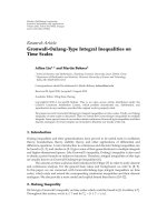
Figure 2: Maximum principal angle of the fast CPAST algorithm in
the first simulation scenario.
signal subspace. Once this estimate is obtained, it can be
used in the DOA estimation algorithm for finding the desired
DOA’s. So, we investigate the performance of fast CPAST in
estimating the signal subspace and compare it with other
subspace tracking algorithms.
The subspace tracking algorithms used in our simu-
lations and their complexities are shown in Tabl e 6.The
Karasalo [1] algorithm is based on subspace averaging.
OPAST is the orthonormal version of PAST proposed
by Abed-Meriam et al. [13]. The BISVD algorithms are
introduced by Strobach [14] and are based on bi-iteration.
PROTEUS and PC are the algorithms developed by Cham-
pagne and Liu [15, 16] and are based on perturbation theory.
NIC is based on a novel information criterion proposed by
Miao and Hua [12]. API and FAPI which are based on power
EURASIP Journal on Advances in Signal Processing 9
Fast CPAST and KARASALO
−1
0
1
2
3

Max. principal angle ratio (dB)
0 100 200 300 400 500 600
Snapshots
(a)
Fast CPAST and PAST
−10
−5
0
5
Max. principal angle ratio (dB)
0 100 200 300 400 500 600
Snapshots
(b)
Fast CPAST and PC
−30
−20
−10
0
10
Max. principal angle ratio (dB)
0 100 200 300 400 500 600
Snapshots
(c)
Fast CPAST and FAST
−10
−5
0
5
10
Max. principal angle ratio (dB)

0 100 200 300 400 500 600
Snapshots
(d)
Ratio between CPAST2 and BISVD1
−6
−4
−2
0
2
Max. principal angle ratio (dB)
0 100 200 300 400 500 600
Snapshots
(e)
Ratio between CPAST2 and BISVD2
−20
−15
−10
−5
0
Max. principal angle ratio (dB)
0 100 200 300 400 500 600
Snapshots
(f)
Fast CPAST and OPAST
−0.5
0
0.5
1
1.5
Max. principal angle ratio (dB)

0 100 200 300 400 500 600
Snapshots
(g)
Ratio between CPAST2 and NIC
−4
−3
−2
−1
0
1
Max. principal angle ratio (dB)
0 100 200 300 400 500 600
Snapshots
(h)
Figure 3: Continued.
10 EURASIP Journal on Advances in Signal Processing
Fast CPAST and PROTEUS1
−15
−10
−5
0
5
Max. principal angle ratio (dB)
0 100 200 300 400 500 600
Snapshots
(i)
Fast CPAST and PROTEUS2
−15
−10
−5

0
5
10
Max. principal angle ratio (dB)
0 100 200 300 400 500 600
Snapshots
(j)
Fast CPAST and API
−4
−3
−2
−1
0
1
Max. principal angle ratio (dB)
0 100 200 300 400 500 600
Snapshots
(k)
Fast CPAST and FAPI
−3
−2
−1
0
1
Max. principal angle ratio (dB)
0 100 200 300 400 500 600
Snapshots
(l)
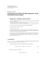
Figure 3: Ratio of maximum principal angles of fast CPAST and other algorithms in the first simulation scenario.
−80

−60
−40
−20
0
20
40
60
80
DOA (deg)
0 100 200 300 400 500 600
Snapshots
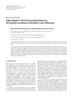
Figure 4: The trajectories of sources in the second simulation
scenario.
iteration are introduced by Badeau et al. [17, 18]. The FAST
algorithm is proposed by Real et al. [19].
In the following subsections the performance of the
fast CPAST algorithm is investigated using simulations. In
Section 7.1, the performance of fast CPAST is compared
with the algorithms mentioned in Ta ble 6 in several cases. In
Table 6: Subspace tracking algorithms used in the simulations and
their complexities.
Algorithm Cost (MAC count)
Fast CPAST 4nr +2r +5r
2
KARASALO nr
2
+3nr +2n + O(r
2
)+O(r
3

)
PAST 3nr +2r
2
+ O(r)
BISVD1 nr
2
+3nr +2n + O(r
2
)+O(r
3
)
BISVD2 4nr +2n + O(r
2
)+O(r
3
)
OPAST 4nr + n +2r
2
+ O(r)
NIC 5nr + O(r)+O(r
2
)
PROTEUS1 (3/4)nr
2
+(15/4)nr + O(n)+O(r)+O(r
2
)
PROTEUS2 (21/4)nr + O(n)+O(r)+O(r
2
)

API nr
2
+3nr + n + O(r
2
)+O(r
3
)
FAPI 3nr +2n +5r
2
+ O(r
3
)
PC 5nr + O(n)
FAST Nr
2
+10nr +2n +64+O(r
2
)+O(r
3
)
Section 7.2,effect of nonstationarity and the parameters n
and SNR on the performance of the fast CPAST algorithm is
investigated. In Section 7.3, the performance of the proposed
signal subspace rank estimator is investigated. In Section 7.4,
the case that we have an abrupt change in the signal DOA is
considered and the performance of the proposed fast CPAST
EURASIP Journal on Advances in Signal Processing 11
Fast CPAST and KARASALO
−4
−2

0
2
Max. principal angle ratio (dB)
0 100 200 300 400 500 600
Snapshots
(a)
Fast CPAST and OPAST
−20
−15
−10
−5
0
Max. principal angle ratio (dB)
0 100 200 300 400 500 600
Snapshots
(b)
Fast CPAST and NIC
−3
−2
−1
0
1
2
Max. principal angle ratio (dB)
0 100 200 300 400 500 600
Snapshots
(c)
Fast CPAST and FAST
−18
−16

−14
−12
−10
Max. principal angle ratio (dB)
0 100 200 300 400 500 600
Snapshots
(d)
Figure 5: Ratio of maximum principal angles of fast CPAST and several other algorithms in the second simulation scenario.
algorithm with truncated window is compared with that of
fast CPAST algorithm with exponential window.
In all simulations of this subsection, we have used the
Monte Carlo simulation and the number of simulation runs
used for obtaining each point is equal to 100. The only
exceptions are Section 7.3 and part 4 in Section 7.2 where the
results are obtained using one simulation run.
7.1. Comparison of the Performance of Fast CPAST with
That of Other Algorithms. In this subsection, we consider a
uniform linear array where the number of sensors is n
= 17
and the distance between adjacent sensors is equal to half
wavelength. In each scenario, an appropriate value is selected
for the forgetting factor. In stationary case, old data could
be useful. So, large values of forgetting factor (β
= 0.99) are
used. On the other hand, in nonstationary scenario where
old data are not reliable, smaller values (β
= 0.75) are used.
Generally, the value selected for the forgetting factor should
depend on the variation of data and improper choosing
of forgetting factor can degrade the performance of the

algorithm.
In the first scenario, the test signal is the sum of signals
of two sources plus a white Gaussian noise. The SNR of each
source is equal to 10 dB. Figure 1 shows the trajectories of
these sources. Since this scenario describes a stationary case,
a forgetting factor of β
= 0.99 has been selected.
Figure 2 shows the maximum principal angle of fast
CPAST algorithm in each snapshot. Principal angles [20]
are measures of the difference between the estimated and
real subspaces. The principal angles are zero if the compared
subspaces are identical. In Figure 3, the maximum principal
angle of fast CPAST is compared with other subspace track-
ing algorithms. In comparisons, the ratio of the maximum
principal angles of fast CPAST and the other algorithms are
obtained in decibels using the following relation:
20 log

θ
CPAST
θ
alg

, (62)
where θ
CPAST
and θ
alg
denote the maximum principal angles
of the fast CPAST and any of the algorithms mentioned in

Ta bl e 3, respectively. This figure shows that the performance
of the fast CPAST is much better than the PC, FAST,
BISVD2, PROTEUS1, and PROTEUS2 after the convergence
of algorithms. In addition, it can be seen from this figure that
the fast CPAST has faster convergence rate than the PAST,
BISVD1, NIC, API, and FAPI algorithms.
In the second scenario, we want to investigate the
behavior of the fast CPAST in comparison with other
12 EURASIP Journal on Advances in Signal Processing
Fast CPAST and KARASALO
−1.5
−1
−0.5
0
0.5
1
Max. principal angle ratio (dB)
0 100 200 300 400 500 600
Snapshots
(a)
Fast CPAST and PAST
−2
−1.5
−1
−0.5
0
0.5
Max. principal angle ratio (dB)
0 100 200 300 400 500 600
Snapshots

(b)
Fast CPAST and NIC
−3
−2
−1
0
1
Max. principal angle ratio (dB)
0 100 200 300 400 500 600
Snapshots
(c)
Fast CPAST and PC
−20
−15
−10
−5
0
5
Max. principal angle ratio (dB)
0 100 200 300 400 500 600
Snapshots
(d)
Figure 6: Ratio of maximum principal angles of fast CPAST and several other algorithms in the third simulation scenario.
−350
−300
−250
−200
−150
−100
−50

0
50
Deviation from orthonormality (dB)
0 100 200 300 400 500 600
Snapshots
PAST
Fast CPAST
API
Figure 7: Deviation from orthonormality for three algorithms in
the third scenario.
algorithms in a nonstationary environment. The test signal is
the sum of signals of two sources plus a white Gaussian noise.
Figure 4 shows the trajectories of the sources. Because of the
nonstationarity of the environment, the forgetting factor is
chosen as β
= 0.75. The SNR of each source is equal to
10 dB. The simulation results showed that the performance
of fast CPAST in this scenario is better than most of the
other algorithms mentioned in Ta ble 3 and approximately
the same as few of them. In Figure 5, the ratio of the
maximum principal angle of fast CPAST and some of these
algorithms are shown in dB.
In the third scenario, we consider two sources that are
stationary and are located at [
−5
◦
,5
◦
]. The SNR of each
of them is equal to

−5 dB. In this scenario β was equal to
0.99. The simulation results showed that the performance of
fast CPAST in this scenario is better than some of the other
algorithms mentioned in Tab le 3 after convergence. For other
algorithms of Tab le 3 , fast CPAST has a faster convergence,
but the performances are similar after the convergence. In
Figure 6, the ratio of the maximum principal angle of fast
CPAST and some of these algorithms are shown in dB.
Figure 3 through Figure 6 show that the fast CPAST
outperforms OPAST, BISVD2, BISVD1, NIC, PROTEUS2,
FAPI, and PC algorithms in all three scenarios. In fact,
in comparison with algorithms that have a computational
complexity equal to O(nr
2
)orO(nr), fast CPAST has equal
or better performance in all three scenarios.
EURASIP Journal on Advances in Signal Processing 13
0
10
20
30
40
50
60
70
80
90
Mean of maximum principal angle (deg)
−30 −20 −10 0 10 20 30
SNR (dB)

Figure 8: Mean of maximum principal angle versus SNR for two
stationary sources located at [
−50
◦
,50
◦
].
0
10
20
30
40
50
60
70
Mean of maximum principal angle (deg)
0102030405060
Number of sensors (n)
Figure 9: Mean of maximum principal angle versus number of sen-
sors for five stationary sources located at [
−10
◦
, −5
◦
,0
◦
,5
◦
,10
◦

].
The deviation of the subspace weighting matrix W(t)
from orthonormality can be measured by means of the
following error criterion [18]:
20 log




W
H
(
t
)
W
(
t
)
−I
r



F

. (63)
We consider the third scenario for investigating the devi-
ation of the subspace weighting matrix from orthonormality.
Ta bl e 7 shows the average of orthonormality error given by
(63) for algorithms in Ta ble 6.ItcanbeseenfromTabl e 7

that fast CPAST, KARASALO, OPAST, BISVD1, PROTEUS2,
FAPI, FAST, API, and PROTEUS1 outperform the other
algorithms. In addition, a plot of variations of the orthonor-
mality error with time (snapshot number) is provided in
Figure 7 for the fast CPAST, API, and PAST algorithms. The
Table 7: Average of orthonormality error given by (63)for
algorithms mentioned in Ta ble 6 in the third simulation scenario.
Algorithm Orthonormality error
fast CPAST, KARASALO, OPAST, BISVD1, about −300 dB
PROTEUS2, FAPI, FAST about
−300 dB
API about
−285 dB
PROTEUS1 about
−265 dB
PAST, NIC about
−30 dB
PC about 0 dB
BISVD2 about 30 dB
−30
−20
−10
0
10
20
30
DOA (deg)
0 100 200 300 400 500
Snapshots
Figure 10: Real trajectories of three crossing-over targets versus

number of snapshots.
results for other algorithms are not presented here to keep
the presentation as concise as possible.
7.2. Effect of SNR, n, and Nonstationarity on the Performance
of the Fast CPAST Algorithm. In this section, we consider a
uniform linear array where the number of sensors is n
=
17 and the distance between adjacent sensors is equal to
half wavelength. The exceptions are Sections 7.2.2 and 7.2.3
where we change the number of sensors.
7.2.1. Effect of the SNR. In this part of Section 7.2,we
investigate the influence of SNR on the performance of the
fast CPAST algorithm. We consider two sources that are
stationary and are located at [
−50
◦
,50
◦
]. The performance
is evaluated for SNR’s from
−30 dB to 30 dB. Figure 8
shows the mean of maximum principal angle for each SNR.
Simulations using fast CPAST and MUSIC showed that for a
SNR of
−10 dB a mean square error of about 1 degree can be
reached in DOA estimation.
7.2.2. Effect of the Number of Sensors. In this part, the effect
of increasing number of sensors on the performance of fast
14 EURASIP Journal on Advances in Signal Processing
−30

−20
−10
0
10
20
30
DOA (deg)
0 100 200 300 400 500
Snapshots
Figure 11: Estimated trajectories of the three crossing-over targets
versus number of snapshots.
0
1
2
3
4
5
6
7
8
9
10
Real or estimated number of sources
0 500 1000 1500
Snapshots
Real number of sources
AIC
MDL
Proposed algorithm
Figure 12: Real and Estimated number of sources versus number of

snapshots.
CPAST is investigated. To do so, we consider five sources that
are stationary and are located at [
−10
◦
, −5
◦
,0
◦
,5
◦
,10
◦
]
and their SNR is 5 dB. Figure 9 shows the mean of maximum
principal angle for n
∈{6,7, ,60}. It can be seen that the
subspace estimation algorithm reaches its best performance
for n
≥ 18 and it remains approximately unchanged with
increasing n.
7.2.3. Effect of a Nonstationary Environment. In this part,
we use MUSIC algorithm for finding the DOA’s of signal
sources impinging on an array of sensors. Let
{s
i
}
n
i
=1

denote
the orthonormal eigenvectors of covariance matrix R. We
assume that the corresponding eigenvalues of R are sorted
in descending order. We know that the MUSIC method
0
10
20
30
40
50
60
70
80
90
0 200 400 600 800 1000
Snapshots
Exponential window
Truncated window
Figure 13: Maximum principal angle of the fast CPAST algorithm
with exponential and truncated windows.
gives consistent estimates of the DOA’s as the minimizing
arguments of the following cost function:
f
MUSIC
(
θ
)
= a
H
(

θ
)

I
n
−SS
H

a
(
θ
)
, (64)
where S is any orthonormal basis of the signal subspace like
S
= (s
1
, , s
r
), and a(θ) is the steering vector corresponding
to the angle θ.
To demonstrate the capability of the proposed algorithm
in target tracking in nonstationary environments, we con-
sider three targets which have crossover in their trajectories.
The trajectories of these three targets are depicted in
Figure 10. The SNR for each of the three targets is equal
to 0 dB and the number of sensors is 17. We have used
the fast CPAST algorithm for tracking the signal subspace
of these targets, the MUSIC algorithm for estimating their
DOA’s, and the Kalman filter for tracking their trajectories.

The simulation result is shown in Figure 11.Itcanbeseen
from Figures 9 and 10 that the combination of fast CPAST,
MUSIC, and Kalman filter algorithms has been successful in
estimating and tracking the trajectories of the sources.
7.3. Performance of the Proposed Signal Subspace Rank
Estimator. In this subsection, we investigate the performance
of the proposed signal subspace rank estimator. To this end,
we consider the case that we have two sources at first, and
then two other sources are added to them at 300th snapshot.
Then, at 900th snapshot two of these sources are removed.
Finally, at 1200th snapshot, another one of the sources is
removed. In this simulation, we assume that α
= 2.5and
r
max
= 6. Figure 12 shows the performance of AIC, MDL,
and the proposed algorithm in tracking number of sources.
It can be seen that the proposed algorithm is successful
in tracking the number of sources. In addition, when the
number of sources decreases, the proposed rank estimator
can track the changes in the number of sources faster than
AIC and MDL.
EURASIP Journal on Advances in Signal Processing 15
0
10
20
30
40
50
60

70
80
90
Maximum principal angle (deg)
0 100 200 300 400 500 600 700 800 900 1000
Snapshots
SWASVD3
Tr un ca te d f as t CPA ST
Figure 14: Maximum principal angle of the truncated fast CPAST
and SWASVD3 algorithms.
7.4. Performance of the Proposed Fast CPAST Algorithm with
Truncated Window. In this section, we compare the conver-
gence behavior of the CPAST algorithm with exponential
and truncated windows. We consider a source whose DOA
is equal to 10
◦
until 300th snapshot and it changes abruptly
to 70
◦
at this snapshot. We assume that the SNR is 10 dB
and the forgetting factor is equal to 0.99. Figure 13 shows
the maximum principal angle of the CPAST algorithm with
exponential and truncated windows. It shows that, in this
case, the CPAST algorithm with truncated window and an
equivalent window length l
= 1/(1 − β), converges much
faster than the exponential window algorithm.
In order to do more investigation about the performance
of truncated fast CPAST algorithm, we have compared its
performance with that of SWASVD3 [21] algorithm which

uses a truncated window for signal subspace tracking. The
scenario that is used in this performance comparison is
the same as that of Figure 13 and the length of window
is equal to 100 for both algorithms. Figure 14 depicts the
result and it can be seen from this figure that the perfor-
mance of the truncated fast CPAST is superior to that of
SWASVD3.
8. Concluding Remarks
In this paper, we introduced an interpretation of the signal
subspace as the solution of a constrained optimization
problem. We derived the solution of this problem and dis-
cussed the applicability of the so-called CPAST algorithm for
tracking the subspace. In addition, we derived two recursive
formulations of this solution for adaptive implementation.
This solution and its recursive implementations avoid the
orthonormalization of basis in each update. The computa-
tional complexity of one of these algorithms (fast CPAST) is
O(nr) which is appropriate for online implementation. The
proposed algorithms are efficiently applicable in those post
processing applications which need an orthonormal basis for
the signal subspace.
In order to compare the performance of the proposed fast
CPAST algorithm with other subspace tracking algorithms,
several simulation scenarios were considered. The simulation
results showed that the performance of fast CPAST is usually
better than or at least similar to that of other algorithms. In
a second set of simulations, effect of SNR, space dimension
n, and nonstationarity on the performance of fast CPAST
was investigated. The simulation results showed good per-
formance of fast CPAST with low SNR and nonstationary

environment.
References
[1] I. Karasalo, “Estimating the covariance matrix by signal
subspace averaging,” IEEE Transactions on Acoustics, Speech,
and Signal Processing, vol. 34, no. 1, pp. 8–12, 1986.
[2] D. J. Rabideau, “Fast, rank adaptive subspace tracking and
applications,” IEEE Transactions on Signal Processing, vol. 44,
no. 9, pp. 2229–2244, 1996.
[3] E.M.Dowling,L.P.Ammann,andR.D.DeGroat,“ATQR-
iteration based adaptive SVD for real time angle and frequency
tracking,” IEEE Transactions on Signal Processing,vol.42,no.4,
pp. 914–926, 1994.
[4] M. Moonen, P. Van Dooren, and J. Vandewalle, “A singular
value decomposition updating algorithm for subspace track-
ing,” SIAM Journal on Matrix Analysis and Applications, vol.
13, no. 4, pp. 1015–1038, 1992.
[5] Y. Hua, Y. Xiang, T. Chen, K. Abed-Meraim, and Y. Miao, “A
new look at the power method for fast subspace tracking,”
DigitalSignalProcessing, vol. 9, no. 4, pp. 297–314, 1999.
[6] C. H. Bischof and G. M. Shroff, “On updating signal
subspaces,” IEEE Transactions on Signal Processing, vol. 40, no.
1, pp. 96–105, 1992.
[7] G. W. Stewart, “An updating algorithm for subspace tracking,”
IEEE Transactions on Signal Processing, vol. 40, no. 6, pp. 1535–
1541, 1992.
[8] G. Xu, H. Zha, G. H. Golub, and T. Kailath, “Fast algorithms
for updating signal subspaces,” IEEE Transactions on Circuits
and Systems II, vol. 41, no. 8, pp. 537–549, 1994.
[9] J. R. Bunch, C. P. Nielsen, and D. C. Sorensen, “Rank-one
modification of the symmetric eigenproblem,” Numerische

Mathematik, vol. 31, no. 1, pp. 31–48, 1978.
[10] R. D. DeGroat, “Noniterative subspace tracking,” IEEE Trans-
actionsonSignalProcessing, vol. 40, no. 3, pp. 571–577, 1992.
[11] B. Yang, “Projection approximation subspace tracking,” IEEE
Transaction on Sig nal Processing, vol. 43, no. 1, pp. 95–107,
1995.
[12] Y. Miao and Y. Hua, “Fast subspace tracking and neural
network learning by a novel information criterion,” IEEE
Transactions on Signal Processing, vol. 46, no. 7, pp. 1967–1979,
1998.
[13] K. Abed-Meraim, A. Chkeif, and Y. Hua, “Fast orthonormal
PAST algorithm,” IEEE Signal Processing Letters, vol. 7, no. 3,
pp. 60–62, 2000.
[14] P. Strobach, “Bi-iteration SVD subspace tracking algorithms,”
IEEE Transactions on Signal Processing, vol. 45, no. 5, pp. 1222–
1240, 1997.
[15] B. Champagne and Q G. Liu, “Plane rotation-based EVD
updating schemes for efficient subspace tracking,” IEEE Trans-
actions on Signal Processing, vol. 46, no. 7, pp. 1886–1900,
1998.
16 EURASIP Journal on Advances in Signal Processing
[16] B. Champagne, “Adaptive eigendecomposition of data covari-
ance matrices based on first-order perturbations,” IEEE Trans-
actions on Signal Processing, vol. 42, no. 10, pp. 2758–2770,
1994.
[17] R. Badeau, B. David, and G. Richard, “Fast approximated
power iteration subspace tracking,” IEEE Transactions on
Signal Processing, vol. 53, no. 8, pp. 2931–2941, 2005.
[18] R. Badeau, G. Richard, and B. David, “Approximated power
iterations for fast subspace tracking,” in Proceedings of the

7th International Symposium on Signal Processing and Its
Applications (ISSPA ’03), vol. 2, pp. 583–586, Paris, France,
July 2003.
[19] E. C. Real, D. W. Tufts, and J. W. Cooley, “Two algorithms
for fast approximate subspace tracking,” IEEE Transactions on
Signal Processing, vol. 47, no. 7, pp. 1936–1945, 1999.
[20] G. H. Golub and C. F. Van Loan, Matr ix Computations, Johns
Hopkins University Press, Baltimore, Md, USA, 2nd edition,
1989.
[21] R. Badeau, G. Richard, and B. David, “Sliding window adap-
tive SVD algorithms,” IEEE Transactions on Signal Processing,
vol. 52, no. 1, pp. 1–10, 2004.