Báo cáo hóa học: " Research Article Rate-Distortion Optimization for Stereoscopic Video Streaming with Unequal Error Protection" ppt

Hindawi Publishing Corporation
EURASIP Journal on Advances in Signal Processing
Volume 2009, Article ID 632545, 14 pages
doi:10.1155/2009/632545
Research Article
Rate-Distortion Optimization for Stereoscopic Video Streaming
with Unequal Error Protection
A. Serdar Tan,
1
Anil Aksay,
2
Gozde Bozdagi Akar,
2
and Erdal Arikan
1
1
Department of Electrical and Electronics Engineering, Bilkent University, 06800 Ankara, Turkey
2
Department of Electrical and Electronics Engineering, Middle East Technical University, 06531 Ankara, Turkey
Correspondence should be addressed to A. Serdar Tan,
Received 1 October 2007; Revised 7 February 2008; Accepted 27 March 2008
Recommended by Aljoscha Smolic
We consider an error-resilient stereoscopic streaming system that uses an H.264-based multiview video codec and a rateless Raptor
code for recovery from packet losses. One aim of the present work is to suggest a heuristic methodology for modeling the end-to-
end rate-distortion (RD) characteristic of such a system. Another aim is to show how to make use of such a model to optimally
select the parameters of the video codec and the Raptor code to minimize the overall distortion. Specifically, the proposed system
models the RD curve of video encoder and performance of channel codec to jointly derive the optimal encoder bit rates and
unequal error protection (UEP) rates specific to the layered stereoscopic video streaming. We define analytical RD curve modeling
for each layer that includes the interdependency of these layers. A heuristic analytical model of the performance of Raptor codes is
also defined. Furthermore, the distortion on the stereoscopic video quality caused by packet losses is estimated. Finally, analytical
models and estimated single-packet loss distortions are used to minimize the end-to-end distortion and to obtain optimal encoder

bit rates and UEP rates. The simulation results clearly demonstrate the significant quality gain against the nonoptimized schemes.
Copyright © 2009 A. Serdar Tan et al. This is an open access article distributed under the Creative Commons Attribution License,
which permits unrestricted use, distribution, and reproduction in any medium, provided the original work is properly cited.
1. Introduction
The recent increase in interest for stereoscopic display
systems and their growing deployment have spurred further
research on efficient stereoscopic video streaming systems.
Stereoscopic video is formed by the simultaneous capture
of two video sequences corresponding to the left and right
views of human visual system, which increases the amount
of source data. Existing stereoscopic techniques compress the
data by exploiting the dependency between the left and right
views; however, the compressed video is more sensitive to
data losses and needs added protection against transmission
errors. To make matters more complicated, the rate of packet
losses in the transmission channel is typically time varying.
Hence, one faces a difficult joint source-channel coding
problem, where the goal is to find the optimal balance
between the distortion created by lossy source compression
and the distortion caused by packet losses in the transmission
channel. In this paper, we address this problem by (i)
proposing a heuristic methodology for modeling the end-to-
end RD characteristic of such a system, and (ii) dynamically
adjusting the source compression ratio in response to
channel conditions so as to minimize the overall distortion.
As opposed to stereoscopic video streaming, various
studies exist in the literature for layered or nonlayered
monoscopic video on optimal rate allocation and error
resilient streaming on error prone channels such as packet
erasure channel (PEC). The early studies on monoscopic

video streaming mainly concentrate on nonlayered video
and the optimal bit control and bit rate allocation for the
video elements [1–4]. RD optimization is the most widely
used optimization method for the quality of video, and it
is a mechanism that aims to calculate optimal redundancy
injection rate into the network, while adapting the video bit
rate accordingly in order to match the available bandwidth
estimate. Redundancy may be generated by means of either
retransmissions or forward error correction (FEC) codes,
and this redundancy is used to minimize the average
distortion resulting from network losses during a streaming
session [5–8]. Even though retransmission methods can be
2 EURASIP Journal on Advances in Signal Processing
Cam.1
Cam.2
Video
enc.
Modeling & joint optimization
R
I
R
L
R
R
Raptor enc. 1
Raptor enc. 2
Raptor enc. 3
R
I
(1 + ρ

I
)
R
L
(1 + ρ
L
)
R
R
(1 + ρ
R
)
(R
C
, p
e
)
Raptor dec. 1
Raptor dec. 2
Raptor dec. 3
Video
dec.
Stereoscopic
display
Figure 1: Overview of the stereoscopic streaming system.
used in video streaming applications as in [9], it may bring
large latency for video display. On the other hand, FEC
schemes insert protection before the transmission and do
not utilize retransmissions. In literature, FEC methods are
studied for video streaming as in [10–12].

A novel technique that recently becomes popular for
error protection in lossy packet networks is Fountain codes,
also called rateless codes. The Fountain coding idea is
proposed in [13] and followed by practical realizations such
as LT codes [14], online codes [15], and Raptor codes [16].
Following the practical realizations, Fountain codes have
gained attention in video streaming in recent years [17–19].
The main idea behind Fountain coding is to produce as many
parity packets as needed on the fly. This approach is different
from the general idea of FEC codes where channel encoding
is performed for a fixed channel rate and all encoded packets
are generated prior to transmission. The idea is proven to be
efficient in [14] for large source data sizes, as in the case of
video data, and it does not utilize retransmissions.
Due to a more intense prediction structure, stereoscopic
video, the main focus of this work is more prone to packet
losses compared to monoscopic video. Interdependent cod-
ing among views may result in quality distortion for both
views if a packet from one view is lost. Even though FEC
codes and optimal bit rate allocations are studied in depth
for monoscopic video streaming, only few studies exist
for stereoscopic video streaming [20]. In [20], stereoscopic
video is layered using data partitioning, but an FEC method
specific to stereoscopic video is not used. In our work, we aim
at filling the gap in the literature on optimal error resilient
streaming of stereoscopic video.
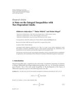
An overview of our proposed stereoscopic streaming
system is presented in Figure 1. Initially, the scene of interest
has to be captured with two cameras to obtain the raw
stereoscopic video data. The video capture process is not

in the scope of our work, thus we use publicly available
raw video sequences. We encode the raw stereoscopic video
data with an H.264-based multiview video encoder. We use
the codec in stereoscopic mode and generate three layers
which are denoted with the symbols I, L,andR. I-frames
are the intracoded frames of the left view; L and R-frames
are the intercoded frames of the left view and right view.
The video encoder can encode each layer with different
quantization parameters, thus with different bit rates R
I
, R
L
,
and R
R
. Due to lossy compression, the encoding process
causes a distortion of D
e
in the video quality. After the
stereoscopic encoder, we apply FEC to each layer separately
where we use Raptor codes as the FEC scheme. The channel
of interest in our system is a packet erasure channel of loss
rate p
e
, and the available bandwidth of the channel is R
C
.
We apply di fferent protection rates ρ
I
, ρ

L
,andρ
R
to each
layer because they contribute differently to the video quality.
After the lossy transmission, some of the packets are lost
and Raptor decoder operates to recover the losses. However,
some packets still may not be recovered, and the loss of these
packets causes a distortion of D
loss
in the video quality. In this
system, our goal is to obtain the optimal values of encoder
bit rates R
I
, R
L
,andR
R
and protection rates ρ
I
, ρ
L
,andρ
R
by
minimizing the total distortion D
tot
 (D
e
+D

loss
). In order to
execute the minimization, we obtain the analytical models of
each part of our system. We start with the modeling of the RD
curve of each layer of the stereoscopic video encoder. Then,
we define the analytical model of the performance of Raptor
codes. Finally, we estimate the distortion on the stereoscopic
video quality caused by packet losses.
The organization of this paper is as follows. In Section 2,
we describe the stereoscopic codec and define the layers of
the stereoscopic video. In Section 3, we present the analytical
model of the RD curve of the video encoder for each of
the layers. In Section 4, we describe the Fountain codes
and describe Raptor codes and their systematization. In
Section 5, we define the analytical model of the Raptor
coding performance curve. Then, in Section 6, we estimate
the distortion caused by the loss of network abstraction
layer (NAL) units. In Section 7, we minimize the total
distortion, which includes both encoder and transmission
distortions, in order to obtain the optimal encoder bit rates
and UEP rates. We also evaluate the performance of the
system and demonstrate its significant quality improvement
on stereoscopic video. Finally, in Section 8,weconcludeand
state possible future work.
2. Stereoscopic Codec
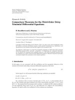
The general structure of a stereoscopic encoder and decoder
is given in Figure 2. In order to maintain backward com-
patibility to monoscopic decoders, left frames are encoded
with prediction only from left frames, whereas right frames
are predicted using both left and right frames. This enables

standard monoscopic decoders to decode left frames.
EURASIP Journal on Advances in Signal Processing 3
Source
left frame
Left
frames
Left frame
encoder
Encoded
left frame
Decoded
picture
buffer
Source
right frame
Right
frames
Right frame
encoder
Encoded
right frame
Stereo encoder
Left frame
decoder
Encoded
left frame
Left
frames
Right
frames

Decoded
picture
buffer
Decoded
left frame
Decoded
right frame
Right frame
decoder
Encoded
right frame
Stereo decoder
Figure 2: Stereoscopic encoder and decoder structure.
Any video codec with this basic structure can be used
with the proposed streaming system in this work. Multiview
extension of H.264 standard [21] (JMVM software) is one of
the candidate codecs for this work. However, hierarchical B-
picture coding used in this codec increases the complexity.
In order to decrease complexity and simplify decoding
procedure, we have used [22], which is a multiview video
codec based on H.264. This codec is an extension of standard
H.264 with the structure given in Figure 2.Inthiscodec,B
frames are not supported. However, the results can easily be
extended for JMVM codec.
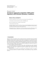
The referencing structure of the codec in [22]isgiven
in Figure 3, where we set the GOP size to 4. Let I
L
, P
L
,and

P
R
denote the set of I-frames of left view, P-frames of left
views, and P-frames of right views, respectively. The set of
frames can be written in open form as I
L
={I
L1
, I
L5
, },
P
L
={P
L2
, P
L3
, }, P
R
={P
R1
, P
R2
, },whereL and R
indicate the frames of left and right video.
Although this coding scheme is not layered, frames
are not equal in importance. We can classify the frames
according to their contribution to the overall quality and use
them as layers of the video. Since losing an I-frame causes
large distortions due to motion/disparity compensation and

error propagation, I-frames should be protected the most.
Among P-frames, left frames are more important since they
are referred by both left and right frames. According to this
prioritization of the frames, we form three layers as shown in
Figure 3.Layerscanbecodedwithdifferent quality (bit rate)
by using either spatial scaling [23] or quantization. In this
work, we use quantization parameter to adjust the quality of
different layers.
Time
Right
view
Left
view
Layer 2
Layer 1
Layer 0
P
R1
P
R2
P
R3
P
R4
P
R5
P
R6
P
L2

P
L3
P
L4
P
L6
I
L1
I
L5
Figure 3: Layers of stereoscopic video and referencing structure.
In the case of slice losses in transmission, we employ dif-
ferent error concealment techniques for different layers in the
decoder. For layer 0, since there is no motion estimation, we
use spatial concealment based on weighted pixel averaging
[24]. For layer 1, we use temporal concealment. Colocated
block from the previous layer-1 frame is used in place of
the lost block. For layer 2, we use temporal concealment
but with a slight modification. In this case, colocated block
can be taken either from previous layer-2 frame or from
the layer-1 frame from the sametime index. Depending on
the neighboring blocks motion vectors, appropriate frame is
selected and colocated block from the selected frame is used
in the place of the lost block.
3. Analytical Model of the RD Curve of
Encoded Stereoscopic Video
In this section, we model the RD curve of stereoscopic video
(D
e
defined in Section 1). The RD curve of video is widely

used for optimal streaming purposes [5–8], which provides
the optimal streaming bit rate for a given distortion in
video quality and vice versa. In [25], a simple analytical RD
curve model that can accurately approximate a wide range of
monoscopic video sequences is presented. The model in [25]
has the form
D
e
(R) =
θ
R − R
0
+ D
0,
(1)
where D
e
(R) is the mean-squared error (MSE) at the video
encoder output at the encoding rate of R bits/sec. There are
3 parameters to be solved which are θ, R
0
,andD
0
.The
parameters R
0
and D
0
do not correspond to any rate or
distortion values and they are not initial values. At least,

three samples of the RD curve are required to solve for the
parameters.
The proposed analytical model in (1)canbeusedforeach
layer of video separately as stated in [25]. However, the model
is not suitable for the cases when the layers are dependent.
In our experiments, when we applied the analytical model
4 EURASIP Journal on Advances in Signal Processing
in (1) separately to each one of our layers, we observed that
the models were not accurate enough to approximate the RD
curve. Thus, the analytical models had to be modified for
dependent layers.
In our work, we have extended the analytical RD model
of monoscopic video proposed in [25] to stereoscopic case
and modified the model to handle the dependency among
the layers. The structure of the layers of our stereoscopic
codec is described in Section 2 and presented in Figure 3.
The primary layer is layer 0 (I-frame) which consists of
intraframes and it does not depend on any previous frames.
Thus, the distortion of layer 0 only depends on the encoder
bit rate of layer 0. The second layer is layer 1 whose frames
are coded dependent on previous frames of layer 1 and layer
0. Thus, the distortion of layer 1 depends on the encoder bit
rates of layer 1 and layer 0. The third layer is layer 2 whose
frames are coded dependent on previous frames of layer 2,
layer 1, and layer 0. Thus, the encoder distortion of layer 2
depends on the encoder bit rates of all layers. We modeled the
RD curves of each layer to include the stated dependencies.
3.1. RD Model of Layer 0. The RD curve model of layer
0isgivenin(2). Layer 0 is encoded as an independent
monoscopic video; hence, we model its RD curve using the

same framework as in (1) and set the model as
D
I
e

R
I

=
θ
I
R
I
−R
0I
+ D
0I.
(2)
Here, D
I
e
(R
I
) is the MSE coming from layer 0 when layer
0 is allocated a rate of R
I
bits/sec. The model parameters are
θ
I
, R

0I
,andD
0I
whichhavetobesolved.
3.2. RD Model of Layer 1. The next analytical model is
realized for layer 1 which consists of predicted frames of left
view. As stated previously, the encoder distortion of layer 1
depends on the encoder bit rate of layer 1 and layer 0. We
modify the model in (1) to handle this dependency as
D
L
e

R
L
, R
I

=
θ
L
R
L
+ c
1
R
I
−R
0L
+ D

0L
. (3)
Here, D
L
e
(R
L
, R
I
) is the MSE coming from layer 1 when
layer 1 and layer 0 are allocated the rates of R
L
and R
I
bits/sec,
respectively. The model parameters are θ
L
, c
1
, R
0L
,and
D
0L
which also have to be solved. The term c
1
R
I
in the
denominator is inserted to handle the dependency of the

distortion of layer 1 to layer 0, where the encoder bit rate of
layer 0 is weighted with the parameter c
1
.
3.3. RD Model of Layer 2. The last analytical model is realized
for layer 2 which consists of the frames of right view. Since
the distortion of layer 2 is dependent on all layers, the
analytical model has to include the encoder bit rates of all
layers. We modify the model in (1) to handle this dependency
as
D
R
e
(R
R
, R
L
, R
I
) =
θ
R
R
R
+ c
2
R
I
+ c
3

R
L
−R
0R
+ D
0R
. (4)
Table 1: Encoder RD curve parameters for “Rena” video.
Layer 0
θ
I
R
0I
D
0I
1.605e + 011 6050 −289860
Layer 1
c
1
θ
L
R
0L
D
0L
0.616 3.483e + 013 51858 6142922
Layer 2
c
2
c

3
θ
R
R
0R
D
0R
0.308 0.086 4.535e + 013 50000 4056654
Table 2: Encoder RD curve parameters for “Soccer” video.
Layer 0
θ
I
R
0I
D
0I
2.978e + 011 10249 120330
Layer 1
c
1
θ
L
R
0L
D
0L
0.456 1.513e + 014 −23018 2209000
Layer 2
c
2

c
3
θ
R
R
0R
D
0R
0.333 0.235 1.496e + 014 19482 6003200
Here, D
R
e
(R
R
, R
L
, R
I
) is the MSE coming from layer 2
when layer 2, layer 1, and layer 0 are allocated the rates of R
R
,
R
L
,andR
I
bits/sec, respectively. The model parameters are
θ
R
, c

2
, c
3
, R
0R,
and D
0R
, which also must be solved. The terms
c
2
R
I
and c
3
R
L
in the denominator are inserted to handle
the dependency of layer 2 to layer 0 and layer 1, where the
encoder bit rates of layer 0 and layer 1 are weighted with
parameters c
2
and c
3
.
3.4. Results on RD Modeling. In order to construct the
RD curve models of stereoscopic videos, that is, to obtain
the model parameters, we used curve fitting tools. In our
work, we used the stereoscopic videos “Rena” and “Soccer”
explained in Section 7.2 and obtained the RD curve models
of these videos for the analytical models in (2)to(4). We

used a general purpose nonlinear curve fitting tool which
uses the Levenberg-Marquardt method with line search [26].
Before the curve fitting operation, we obtained many RD
curve samples of the video by sweeping the quantization
parameters of each layer from low to high quality. We
obtained more RD samples than required in order to be
able to observe the curve fitting performance. Then, we
chose some of the RD samples and inserted into the curve
fitting tool. The resulting analytical model parameters of the
curve fit process are given in Tables 1 and 2 for the chosen
videos. The parameters are in accordance with the properties
of the videos. “Rena” has static background with moving
objects and “Soccer” has a camera motion. Since the “Soccer”
video has a camera motion, while encoding a right frame,
correlation with the current left frame can be more than the
previous right frame. This shows why the c
3
parameter of
layer 2 of the “Soccer” video is high when compared with
the results of the “Rena” video.
EURASIP Journal on Advances in Signal Processing 5
Rate-distortion curve for layer-0
0
2
4
6
8
10
12
×10

6
Encoder distortion in layer-0 (MSE)
00.511.522.5
×10
5
R
I
(bps)
Analytical model: D
I
e
(R
I
)
RD samples
Figure 4: RD curve for layer 0 of the “Rena” video.
Rate-distortion curve for layer-0
0
0.5
1
1.5
2
2.5
3
3.5
×10
7
Encoder distortion in layer-0 (MSE)
00.511.522.5
×10

5
R
I
(bps)
Analytical model: D
I
e
(R
I
)
RD samples
Figure 5: RD curve for layer 0 of the “Soccer” video.
In Figures 4 to 9, we present the results of analytical
modeling of the RD curves. In Figures 4 and 5,wegive
the results for layer 0, where the analytical models are
constructed using the model in (2) with the corresponding
parameters from Tables 1 and 2. The RD samples correspond
to the actual RD values obtained from the video encoder
before the curve fitting process. Later, the results for layer
1 are presented in Figures 6 and 7 and those of layer 2
are presented in Figures 8 and 9. In the figures for layer
1 and 2, we present two cross-sections of the RD curves.
The cross sections are obtained by fixing the encoder bit
rates of the layers other than the corresponding layer of
Rate-distortion curve for layer-1
0
0.5
1
1.5
2

2.5
3
3.5
×10
8
Encoder distortion in layer-1 (MSE)
00.511.522.5
×10
6
R
L
(bps)
Analytical model: D
L
e
(R
L
, R
I
= 200.7kbps)
RD samples, R
I
= 200.7kbps
Analytical model: D
L
e
(R
L
, R
I

= 24.2kbps)
RD samples, R
I
= 24.2kbps
Figure 6: RD curve for layer 1 of the “Rena” video.
Rate-distortion curve for layer-1
0
1
2
3
4
5
6
7
8
9
×10
8
Encoder distortion in layer-1 (MSE)
00.511.52 2.53
×10
6
R
L
(bps)
Analytical model: D
L
e
(R
L

, R
I
= 222.8kbps)
RD samples, R
I
= 222.8kbps
Analytical model: D
L
e
(R
L
, R
I
= 28 kbps)
RD samples, R
I
= 28 kbps
Figure 7: RD curve for layer 1 of the “Soccer” video.
interest. The average difference between analytical models
and RD samples for the “Rena” video are 3.62%, 7.60%,
and 9.19% for layer 0, 1, and 2, respectively, and those
of the “Soccer” video are 1.00%, 5.87%, and 8.89%. Thus,
for both of the videos, which have different characteristics,
satisfactory results are achieved where the analytical model
approximates the RD samples accurately.
6 EURASIP Journal on Advances in Signal Processing
Rate-distortion curve for layer-2
0
1
2

3
4
5
6
×10
8
Encoder distortion in layer-2 (MSE)
00.511.522.5
×10
6
R
R
(bps)
Analytical model: D
L
e
(R
R
, R
L
= 984.8kbps,R
I
= 200.7kbps)
RD samples, R
L
= 984.8kbps,R
I
= 200.7kbps
Analytical model: D
L

e
(R
R
, R
L
= 157.9kbps,R
I
= 24.2kbps)
RD samples, R
L
= 157.9kbps,R
I
= 24.2kbps
Figure 8: RD curve for layer 2 of the “Rena” video.
Rate-distortion curve for layer-2
0
1
2
3
4
5
6
7
×10
8
Encoder distortion in layer-2 (MSE)
00.511.52 2.53
×10
6
R

R
(bps)
Analytical model: D
L
e
(R
R
, R
L
= 1541.3kbps,R
I
= 222.8kbps)
RD samples, R
L
= 1541.3kbps,R
I
= 222.8kbps
Analytical model: D
L
e
(R
R
, R
L
= 367.3kbps,R
I
= 28 kbps)
RD samples, R
L
= 367.3kbps,R

I
= 28 kbps
Figure 9: RD curve for layer 2 of the “Soccer” video.
4. Raptor Codes
Inourwork,weuseRaptorcodes[16] as the FEC scheme
to protect the encoded stereoscopic video data from the
packet losses during transmission. We choose Raptor codes
due to their low complexity and ease of employability on
packet networks. Raptor codes are the most recent practical
realization of Fountain codes [13]. Fountain codes, also
called rateless codes, are a novel class of FEC codes where
LT c o de
High-rate
pre-code
Output
symbols
Input
symbols
Intermediate
symbols
···
Figure 10: Representation of Raptor encoder.
as many parity packets as needed are generated on the fly.
Fountain codes are low complexity channel codes providing
reliability, low latency, and loss rate adaptability. There are
many practical realizations of fountain codes such as Luby
transform (LT) codes [14], online codes [15], and the most
recent one being Raptor codes. In all of the Fountain coding
schemes the original data is divided into k packets (source
packets) denoted as input symbols. The encoded packets

(transmitted packets) are denoted as output symbols.Anideal
fountain encoder can generate potentially limitless output
symbols in linear complexity and an ideal fountain decoder
can reconstruct the original data in linear complexity if any
k(1 + ε) of the output symbols are received, where ε goes to
zero as k increases.
Raptor codes are an extension of LT codes and their
encoding structure is represented in Figure 10. They have
two consecutive channel encoders, where the precode is
a high-rate FEC code and the outercode is an LT code.
Input symbols are the data units of the original source
data. An input symbol can be a bit or a symbol composed
of s bits. In our work, each NAL unit generated by the
stereoscopic video encoder corresponds to an input symbol.
The precode generates intermediate symbols which are not
transmitted but are used as an intermediate step to generate
the transmitted output symbols. The precode is presented to
reduce the overhead of LT codes. LDPC codes [27] are the
most commonly used FEC codes as the precode on Raptor
codes.
In the following, we define the input output relations
for the Raptor coder in our work. For now, assume that
we are given the parity ratio ρ and the bit rate of encoded
video R.LetN
bits
denote the number of bits in a NAL unit,
then the number of input symbols can be defined as N
i
=
R/N

bits
, and the number of output symbols can be calculated
as N
o
= (1 + ρ)N
i
. The Raptor encoder forms N
o
output
symbols which are linear combinations of the input symbols
chosen from a degree distribution. Details on the degree
distributions are given in [16]. The Raptor decoder receives
N
r
out of N
o
of these output symbols after lossy transmission.
Any algorithm that solves for the input symbols using these
N
r
output symbols is a Raptor decoder.
Similartoanylinearblockcode,Raptorcodescan
be systematic or nonsystematic. In systematic codes, the
transmitted symbols consist of the original data symbols
and the parity symbols, whereas in the nonsystematic case
the original data symbols are transformed into new symbols
for transmission. The access to original data is beneficial in
EURASIP Journal on Advances in Signal Processing 7
video transmission applications since 100% reliability is not
obliged. When the video data is encoded with systematic

channel codes, even if the channel decoder cannot decode
all of the input symbols, the video decoder can use error
concealment techniques to approximate the lost symbols of
thevideo.Inourwork,weusesystematicRaptorcodes
as the FEC scheme. For our systematic Raptor coding
implementation, we use a practical and low-complexity
scheme described in [28].
5. Analytical Modeling of the Performance
Curve of Raptor Codes
In this section, we model the performance curve of Raptor
codes. The performance curve of Raptor codes is defined as
the graph that represents the average number of undecoded
input symbols versus the number of received output sym-
bols. Thus, we aim at obtaining the analytical model of the
residual number of lost packets after the channel decoder.
5.1. Performance Curve Model. We propose a heuristic
analytical model of the performance curve of Raptor codes
which is going to be used for the derivation of optimal parity
packet allocation to layers in Section 7 in the end-to-end
distortion minimization. We define the analytical model as
N
u

N
i
, N
r
, ρ

=

⎧
⎪
⎪
⎪
⎨
⎪
⎪
⎪
⎩
N
i
−
N
r
(1 + ρ)
, N
r
≤ N
i
,
N
i
ρ
(1 + ρ)
2
(N
i
−N
r
)

, N
r
>N
i
.
(5)
In (5), N
u
(N
i
, N
r
, ρ) is the analytical model of the number
of undecoded input symbols which is a function of N
i
,
N
r
,andρ. In order to form the model, we investigate
the performance curve in two separate regions; first, in
the region with the number of received symbols less than
or equal to number of input symbols and, second, in the
remaining region. In the first region of the model, we assume
that the Raptor decoder cannot decode any lost symbols
other than the received systematic symbols. whereas, in the
second region, an exponential decrease in the number of
undecoded symbols is assumed.
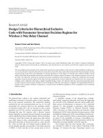
5.2. Results on the Performance Curve Modeling. In Figure 11,
the actual performance curve and the analytical model are
presented for N

i
= 100 and ρ = 0.5. In Figure 12,weprovide
the curves zoomed around N
r
= 100 for the curves given
in Figure 11. In Figures 13 and 14, results with different
parity ratios and different number of input symbols are
presented. In the figures, we provide the actual performance
curve and the analytical model for comparison. We obtain
the actual performance curve as follows. Initially, for given
N
i
and ρ,(1+ρ)N
i
output symbols are created as described
in [28]. Then, randomly N
r
output symbols are selected and
inserted to Raptor decoder and the number of undecoded
input symbols are recorded. For each value of N
r
(1 to
(1 + ρ)N
i
), this process is repeated for 200 times and the
number of undecoded symbols are averaged to obtain the
Number of input symbols: 100, parity ratio: 0.5
0
10
20

30
40
50
60
70
80
90
100
Average number of undecoded symbols
0 20 40 60 80 100 120
Number of received symbols
Actual performance
Analytical model
Figure 11: Performance curve of Raptor coding, N
i
= 100, ρ = 0.5.
Number of input symbols:100,
parity ratio: 0.5(zoomedaroundN
r
= N
i
)
0
5
10
15
20
25
30
35

Average number of undecoded symbols
96 98 100 102 104 106 108
Number of received symbols
Actual performance
Analytical model
Figure 12: Performance curve of Raptor coding (zoomed around
N
r
= N
i
), N
i
= 100, ρ = 0.5.
actual performance. We obtained the analytical model with
(5) by plotting N
u
versus N
r
for given N
i
and ρ.Asobserved
from the figures, the analytical model approximates the
performance curve of Raptor codes accurately.
6. Estimation of Transmission Distortion
In this section, our aim is to estimate the residual loss
distortion in video remaining after the Raptor decoder and
stereoscopic video decoder (D
loss
defined in Section 1). In the
8 EURASIP Journal on Advances in Signal Processing

Number of input symbols: 100, parity ratio: 1
0
10
20
30
40
50
60
70
80
90
100
Average number of undecoded symbols
0 20406080100
120
Number of received symbols
Actual performance
Analytical model
Figure 13: Performance curve of Raptor coding, N
i
= 100, ρ = 1.0.
Number of input symbols: 200, parity ratio: 0.5
0
20
40
60
80
100
120
140

160
180
200
Average number of undecoded symbols
0 50 100 150 200 250
Number of received symbols
Actual performance
Analytical model
Figure 14: Performance curve of Raptor coding, N
i
= 200, ρ = 0.5.
following sections, we explain the estimation of residual loss
distortion step by step.
6.1. Lossy Transmission. The channel of interest in our work
is PEC as mentioned previously. During the transmission
of stereoscopic video layers from PEC, NAL units are lost
with probability p
e
. In the remaining part of our work, for
simplicity, X will represent the layer denotations I, L,and
R. As explained in the system overview in Section 1,we
have three layers of video with source bit rate R
X
which are
Raptor encoded separately with inserted parity rate ρ
X
.Thus,
N
X
i

(1 + ρ
X
) output symbols are created and transmitted for
each layer. After lossy transmission, the number of received
output symbols in Raptor decoder can be calculated as
N
X
r
= N
X
i

1+ρ
X

1 − p
e

. (6)
Here, we use the average loss probability for simpli-
fied modeling purposes only. The experimental results in
Section 7.2 reflect the actual distortions over lossy channels,
where a single packet is lost with probability P
e
.
6.2. Reconstruct ion of Input Symbols in Raptor Decoder. After
receiving N
X
r
output symbols Raptor decoder operates to

solve for the input symbols. We use the model of the
performance curve of Raptor codes to obtain the average
number of undecoded input symbols using (5). The average
number of undecoded input symbols (the residual number
of lost NAL units) can be calculated as
N
X
u
= N
u

N
X
i
, N
X
r
, ρ
X

. (7)
6.3. Propagation of Lost NAL Units in Stereoscopic Video
Decoder. Due to the recursive structure of the video codec,
the distortion of an NAL unit loss not only causes distortion
in the corresponding frame, but it also propagates to
subsequent frames in the video. Initially, since each NAL
unit contains a specific number of macroblocks (MBs), we
estimate the distortion in a frame when a single MB is
lost. The distortion is calculated after error concealment
techniques, explained in Section 2, are applied for the lost

MB. Then, we calculate the average propagated distortion of
a single MB and, consequently, an NAL unit.
In [25], a model for distortion propagation is proposed,
where the propagated error energy (distortion) at frame t
after a loss at frame 0 is given as
σ
2
u
(t) =
σ
2
u0
1+γt
. (8)
Here, σ
2
u0
is the average distortion per lost unit, and γ
is the leakage factor which describes the efficiency of the
loop filtering in the decoder to remove the introduced error
(0 <γ<1). We assume γ
≈ 0 which results in worst case
propagation, where the distortion propagates equally to all
subsequent frames (σ
2
u
(t) = σ
2
u0
). In the following sections,

we calculate the propagated NAL unit loss distortion for each
layer separately, where we set MBs as the video unit.
6.3.1. NAL Unit Loss from Layer 0. The expression in (9)gives
the average distortion of spatial error concealment when
a lost MB is concealed by the average of its neighboring
MBs. In (9), S
MB
,MB
i
, S
MB,i
, N

i
,andN
I
MB
represent the
set of macroblocks, the ith macroblock, the set of ith MB’s
neighbors, the number of neighbors of ith MB, and the
number of MBs of layer 0, respectively. I
I
(x, y, 0) denotes the
pixel in position (x, y) of the intraframe of layer 0. Layer
0 consists of a single intraframe, thus only spatial error
EURASIP Journal on Advances in Signal Processing 9
I
L1
P
L2

P
L3
P
L4
σ
2
I0
σ
2
I0
σ
2
I0
σ
2
I0
σ
2
I0
σ
2
I0
σ
2
I0
σ
2
I0
P
R1

P
R2
P
R3
P
R4
···
···
Figure 15: Propagation of an MB loss from I-frame.
concealment can be used due to intracoding as described in
Section 2:
σ
2
I0
=
1
N
I
MB

k∈S
MB


x,y∈MB
k

I
I
(x, y,0)−


x

,y

∈MB

k
I
I

x

, y

,0

/N

k

2

.
(9)
In Figure 15, the propagation of an MB loss in an I-frame
is demonstrated. The black box in the frame I
L1
represents a
possible loss in the I-frame. The loss causes a distortion of σ

2
I0
as calculated in (9) for the frame I
L1
. The loss propagates to
all subsequent frames with equal distortion on the average
since both L-frames and R-frames refer initially to the I-
frame. If we denote the GOP size as T, then the average of
total propagated loss distortion when an MB is lost from layer
0 can be calculated as
D
I
MB prop
= 2Tσ
2
I0
. (10)
In order to calculate the average distortion of losing an
NAL unit from layer 0 (D
I
NAL loss
), we have to calculate the
average number of MBs in a NAL unit. Let N
I
MB
denote the
number of MBs in layer 0. Then, D
I
NAL loss
can be calculated

as
D
I
NAL loss
=

N
I
MB
N
I
i

·
D
I
MB prop
. (11)
6.3.2. NAL Unit Loss from Layer 1. The expression in (12)
gives the average distortion of temporal error concealment
when a lost NAL unit is concealed from the previous frame
of layer 1. In (12), N
L
MB
and T represent the number of MBs
of layer 1 and GOP size, respectively. I
L
(x, y, i) denotes the
pixel in position (x, y)ofith frame of layer 1. Layer 1 consists
of predicted frames of left view. In our stereoscopic codec, we

used temporal error concealment for layer 1 as described in
Section 2:
σ
2
L0
=

1/(T −1)


T−1
i
=1

x,y

I
L
(x, y, i) − I
L
(x, y, i − 1)

2
N
L
MB
.
(12)
I
L1

P
L2
P
L3
P
L4
σ
2
L0
σ
2
L0
σ
2
L0
1
2
σ
2
L0
3
4
σ
2
L0
7
8
σ
2
L0

P
R1
P
R2
P
R3
P
R4
···
···
Figure 16: Propagation of an MB loss from L-frame.
In Figure 16,thepropagationofanMBlossinanL-frame
is demonstrated. The black box in the frame P
L2
represents
a possible loss in the L-frame. The loss causes a distortion
of σ
2
L0
as calculated in (12) for the frame P
L2
. The loss
propagates to all subsequent L-frames with equal distortion
since each L-frame refers to the previous L-frame. Let m
denote the frame index of loss in a GOP, then the average
propagated loss to L-frames can be calculated as
1
T −1
T−1


m=1
(T −m)σ
2
L0
. (13)
The MB loss also propagates to R-frames. However, R-
frames not only refer to current L-frames but also previous
R-frames. Due to this fact, the distortion in P
R2
can be
calculated as σ
2
L0
/2 using the previous undistorted MB (white
box in P
R1
). In the frame P
R3
the propagated distortion can
be calculated as (σ
2
L0
/2+σ
2
L0
)/2 = (3/4)σ
2
L0
. In the subsequent
frames, the propagated distortion is calculated similarly

as shown in Figure 16. The average of total propagated
distortion in an R-frame caused by the loss of an L-frame
MB can be calculated as
1
T −1
T−1

m=1
T
−m

n=1

1 −
1
2
n

σ
2
L0

. (14)
Thus, the average of total propagated distortion when an
MB is lost from layer 1 can be calculated as
D
L
MB prop
=
1

T −1
T−2

m=0
m

n=0

2 −
1
2
n+1

σ
2
L0

. (15)
In order to calculate the average distortion of losing an
NAL unit from layer 1 (D
L
NAL loss
), we have to calculate the
average number of MBs in an NAL unit. Let N
L
MB
denote the
number of MBs in layer 1. Then, D
L
NAL loss

can be calculated
as
D
L
NAL loss
=

N
L
MB
N
L
i

·
D
L
MB prop
. (16)
6.3.3. NAL Unit Loss from Layer 2. The expression in (17)
gives the average distortion of temporal error concealment
when a lost NAL unit is concealed from the frames of layer 2
and layer 1. In (17), N
R
MB
and T represent the number of MBs
of layer 2 and GOP size, respectively. I
R
(x, y, i) denotes the
10 EURASIP Journal on Advances in Signal Processing

I
L1
P
L2
P
L3
P
L4
σ
2
R0
1
2
σ
2
R0
1
4
σ
2
R0
P
R1
P
R2
P
R3
P
R4
···

···
Figure 17: Propagation of an MB loss from R-frame.
pixel in position (x, y)ofith frame of layer 2. Layer 2 consists
of predicted frames of right view. In our stereoscopic codec,
we used temporal error concealment for layer 2, where the
frames are referred to previous layer 2 and current layer 1
frames as described in Section 2:
σ
2
R0
=

x,y

I
L
(x, y,0)−I
R
(x, y,0)

2
(T −1)N
R
MB
+

T−1
i
=1


x,y

Q −I
R
(x, y, i)

2
(T −1)N
R
MB
,
(17)
where Q
= ((I
R
(x, y, i − 1) + I
L
(x, y, i))/2).
In Figure 17, the propagation of an MB loss in an R-
frame is demonstrated. The black box in the frame P
R2
represents a possible loss in the R-frame. The loss in an R-
frame propagates only to the subsequent R-frames. A loss in
the frame P
R2
creates a distortion of σ
2
R0
as calculated in (17).
In frame P

R3
, the propagation distortion can be calculated as
σ
2
R0
/2 using the undistorted MB in the L-frame (white box
in P
L3
). In each of the following R-frames, the propagated
distortion is the half of the previous R-frame. Thus, the
average of total propagated distortion when an MB is lost
from layer 2 can be calculated as
D
R
MB prop
=
T−1

m=0
1
T
m

n=0

1
2
n
σ
2

R0

. (18)
In order to calculate the average distortion of losing an
NAL unit from layer 2 (D
R
NAL loss
), we have to calculate the
average number of MBs in an NAL unit. Let N
R
MB
denote the
number of MBs in layer 2. Then, D
R
NAL loss
can be calculated as
D
R
NAL loss
=

N
R
MB
N
R
i

·
D

R
MB prop
. (19)
6.4. Calculation of Residual Loss Distortion. In this part, we
calculate the average transmission distortion after Raptor
decoder and stereoscopic video decoder. Let D
X
loss
denote the
residual transmission distortion. In (20), we calculate D
X
loss
by multiplying the number of undecoded input symbols
with the average distortion of losing an NAL unit:
D
X
loss
(R
X
, ρ
X
, p
e
) = N
u
(N
X
i
, N
X

r
, ρ
X
)·D
X
NAL loss
. (20)
Here, we use the assumption that the NAL unit losses are
uncorrelated which is met for low number of losses after the
Raptor decoder. Thus, the accuracy of the model may reduce
forhighlossrates.
7. End-to-End Distortion Minimization and
Performance Evaluation
As the last part of our system, we minimize the total end-to-
end distortion to find the optimal encoder bit rates and UEP
rates and evaluate the performance of the system. We present
the minimization as
min
(R
I
,R
L
,R
R
,ρ
I
,ρ
L
,ρ
R

)
D
tot
s.t.

1+ρ
I

R
I
+

1+ρ
L

R
L
+

1+ρ
R

R
R
= R
C
.
(21)
The minimization aims at obtaining the optimal encoder
bit rates R

I
, R
L
,andR
R
, and optimal parity ratios ρ
I
, ρ
L
,
and ρ
R
for given p
e
and R
C
. The constraint ensures that the
final bit rate satisfies a total transmission bandwidth of R
C
including both the encoder bit rates and protection data bit
rates. In (22), we present the calculation of D
tot
where D
I
e
(·),
D
L
e
(·), and D

R
e
(·) are the encoder distortions defined in (2),
(3), and (4), and D
I
loss
(·), D
L
loss
(·), and D
R
loss
(·) are the residual
loss distortions defined in (20):
D
tot
=
1
3

D
R
e

R
R
, R
L
, R
I


+ D
R
loss

R
R
, r
r
, p
e


+
2
3

D
I
e

R
I

+ D
L
e

R
L

, R
I

+ D
I
loss

R
I
, ρ
I
, p
e

+ D
L
loss

R
L
, ρ
L
, p
e


.
(22)
Total distortion in left and right frames is weighted to
handle the objective stereoscopic video quality as stated in

[29]. The weighting parameters in [29]arefoundbyleast
squares fitting of the subjective results with the distortion
values. In [29], there are three parameters used for coding,
number of layers, quantization parameter for left view,
and temporal scaling. In our codec, we are only using
quantization parameter for adjusting the bit rates. Although
both codecs are not the same, they are both extensions of
H.264 JM and JSVM softwares. So, the distortions become
similar if we consider only the case where quantization
parameter is used to adjust the bit rates. Also, subjective
results for our codec with temporal and spatial scaling can
be found in [24],wherewehavesimilarresultsgivenin[29].
7.1. Results on the Minimization of End-to-End Distortion.
We solve the minimization in (21)byageneralpurpose
minimization tool which uses sequential quadratic program-
ing where the tool solves a quadratic programing at each
iteration as described in [30]. In our work, we obtain the
optimal encoder bit rates and parity ratios for P
e
∈{0.03,
0.05, 0.1, 0.2
} and R
C
∈{500, 750, 1000, 1500, 2000, 2500
(kbps)
} for“Rena”videoandR
C
∈{1000, 1500, 2000, 2500,
3000, 3500 (kbps)
} for “Soccer” video. Thus, we perform 24

optimizations per video using (21).
In Tables 3 and 4, the optimal encoder bit rates and
protection rates for the proposed method are given for the
“Rena” and “Soccer” stereoscopic videos for p
e
= 0.10. The
encoder bit rates of the right view are lower than that of
the left view, which is caused by the unequal weighting in
the total distortion expression in (22).Theprotectionrateof
EURASIP Journal on Advances in Signal Processing 11
Table 3: Video encoder bit rates and Raptor encoder protection rates for “Rena” video.
P
e
= 0.1
R
C
(Kbps) Encoder bit rates (Kbps) Protection rates
(optimal) Proposed (optimal) EEP Protect-L
R
I
R
L
R
R
ρ
I
ρ
L
ρ
R

ρ
I
ρ
L
ρ
R
ρ
I
ρ
L
ρ
R
500 33.5 216.6 169.8 0.489 0.177 0.147 0.190 0.190 0.190 0.320 0.320 0.000
750
51.5 337.8 250.7 0.389 0.158 0.143 0.172 0.172 0.172 0.282 0.282 0.000
1000
69.6 460.0 332.2 0.332 0.148 0.139 0.160 0.160 0.160 0.260 0.260 0.000
1500
106.0 705.6 496.0 0.270 0.138 0.133 0.147 0.147 0.147 0.237 0.237 0.000
2000
142.4 951.9 660.3 0.236 0.132 0.129 0.140 0.140 0.140 0.224 0.224 0.000
2500
178.9 1198.7 824.8 0.215 0.128 0.127 0.135 0.135 0.135 0.216 0.216 0.000
Table 4: Video encoder bit rates and Raptor encoder protection rates for “Soccer” video.
P
e
= 0.1
R
C
(Kbps) Encoder bit rates (Kbps) Protection rates

(optimal) Proposed (optimal) EEP Protect-L
R
I
R
L
R
R
ρ
I
ρ
L
ρ
R
ρ
I
ρ
L
ρ
R
ρ
I
ρ
L
ρ
R
1000 68.4 543.0 245.9 0.349 0.147 0.156 0.166 0.166 0.166 0.233 0.233 0.000
1500
96.0 833.8 373.7 0.294 0.136 0.145 0.151 0.151 0.151 0.211 0.211 0.000
2000
123.7 1125.3 501.9 0.260 0.130 0.138 0.142 0.142 0.142 0.199 0.199 0.000

2500
151.3 1417.2 630.3 0.238 0.127 0.134 0.137 0.137 0.137 0.192 0.192 0.000
3000
179.0 1709.3 758.7 0.222 0.125 0.131 0.133 0.133 0.133 0.186 0.186 0.000
3500
206.6 2001.6 887.3 0.209 0.123 0.128 0.131 0.131 0.131 0.183 0.183 0.000
I-frame is the largest due to low bit rate and high distortion
of losses.
In Tables 3 and 4, the protection rates of equal error
protection (EEP) and Protect-L cases are also given. These
protection rates are nonoptimal and will be compared with
the proposed optimal protection rates by simulations. In
order to construct the EEP case, the resulting bit rate of
proposed protection is distributed to the layers so that
each layer has the same protection ratio. Protect-L case is
constructed similarly, using the results of [31], where the
bit rate of protection is distributed to only layers of left
view (layer 1 and layer 0) so that these layers have the same
protection ratio. The encoder bit rates for EEP and Protect-L
are the same as the optimal streaming case.
7.2. Simulation Results. In this section, we evaluate the
performance of the proposed stereoscopic video streaming
system on lossy channels via simulations. We use two
stereoscopic videos “Rena” (Camera 38, 39) (640
×480, first
30 frames) and “Soccer” (720
× 480, first 30 frames) for
performance evaluation. We encode the stereoscopic videos
with the bit rates obtained by the minimization in (21)for
given p

e
and R
C
, and NAL unit size is fixed to 150 bytes. The
number of NAL units per layer can be calculated by dividing
the given encoder bit rate to NAL unit size which yields the
number of input symbols for the channel coder.
For channel protection, we use systematic Raptor codes
based on their suitability for our case as explained in
Section 4. We applied Raptor encoding to the source encoded
video data using the protection rates obtained by the mini-
mization in (21)forgivenp
e
and R
C
. The proposed optimal
streaming scheme is compared with EEP, Protect-L, no-loss,
and no-protection cases. The no-loss case represents the
quality of the video when the stereoscopic video is encoded
with all available channel bandwidth and no transmission
occurs. The no-protection case represents the transmission
of the video of no-loss case without any channel protection
and only error concealment is used at the decoder.
The simulation results give the average of 100 indepen-
dent lossy transmission simulations for each p
e
and R
C
,
whereeachpacketislostwithaprobabilityofp

e
. Simulation
results are based on the weighted PSNR measure. If we
denote the average left and right per pixel distortions in MSE
as D
left
and D
right
, then the total PSNR distortion D(dB) can
be calculated as
D (dB)
= 10·log
10

255
2
(2/3)D
left
+(1/3)D
right

. (23)
We give the simulation results of stereoscopic video
pair “Rena” in Figures 18 to 21 and those of “Soccer”
in Figures 22 to 25. The gap between the results of the
no-loss and the proposed case is caused by the reduction
of the encoder bit rates of video where the remaining
bit rate is used for channel protection. The simulation
12 EURASIP Journal on Advances in Signal Processing
p

e
= 0.03
30
32
34
36
38
40
42
PSNR (dB)
0.511.522.5
×10
6
R
C
(bits/s)
Protect-L
EEP
Proposed
No-loss
No-protection
Figure 18: Results for p
e
= 0.03 for “Rena” video.
p
e
= 0.05
30
32
34

36
38
40
42
PSNR (dB)
0.511.522.5
×10
6
R
C
(bits/s)
Protect-L
EEP
Proposed
No-loss
No-protection
Figure 19: Results for p
e
= 0.05 for “Rena” video.
results demonstrate the superiority of the proposed scheme
compared to nonoptimized schemes. For low bit rates, the
difference is not clear but for high bit rates the difference is
1dBfor p
e
= 0.10 and nearly 2 dB for p
e
= 0.20. The results
of the no-protection case clearly point out the need for FEC
utilization in stereoscopic video streaming.
8. Conclusions

In this work, we presented a rate-distortion optimized
error-resilient stereoscopic video streaming system with
Raptor codes and evaluated its performance via simulations.
p
e
= 0.1
26
28
30
32
34
36
38
40
42
PSNR (dB)
0.511.522.5
×10
6
R
C
(bits/s)
Protect-L
EEP
Proposed
No-loss
No-protection
Figure 20: Results for p
e
= 0.10 for “Rena” video.

p
e
= 0.2
26
28
30
32
34
36
38
40
42
PSNR (dB)
0.511.522.5
×10
6
R
C
(bits/s)
Protect-L
EEP
Proposed
No-loss
No-protection
Figure 21: Results for p
e
= 0.20 for “Rena” video.
We investigated all aspects of an end-to-end stereoscopic
streaming system. Initially, we defined the layers of the
stereoscopic video which have interdependencies. Then, we

obtained the analytical models for the RD curve of these
layers where we extended the model of monoscopic video for
the dependent layers of stereoscopic video. We showed that
the analytical model of the RD curve accurately approximates
the actual RD curve of the layers. Then, we obtained the
analytical model of Raptor codes, which also accurately
approximates the actual performance. Then, we estimated
the transmission distortion for each layer where we also
considered the propagation of NAL unit losses to following
EURASIP Journal on Advances in Signal Processing 13
p
e
= 0.03
31
32
33
34
35
36
37
38
39
40
41
PSNR (dB)
11.522.533.5
×10
6
R
C

(bits/s)
Protect-L
EEP
Proposed
No-loss
No-protection
Figure 22: Results for p
e
= 0.03 for “Soccer” video.
p
e
= 0.05
30
32
34
36
38
40
PSNR (dB)
11.522.533.5
×10
6
R
C
(bits/s)
Protect-L
EEP
Proposed
No-loss
No-protection

Figure 23: Results for p
e
= 0.05 for “Soccer” video.
frames. Finally, we combined the two analytical models
and the estimated transmission distortions in an end-to-end
distortion minimization to obtain optimal encoder bit rates
and UEP rates for the defined layers.
We evaluated the performance of the system via simu-
lations where we used two stereoscopic videos “Rena” and
“Soccer,” which have different video characteristics. For both
of the videos, the simulation results yielded the superiority
of the proposed system compared to nonoptimized schemes.
Also, the necessity of the utilization of FEC codes, such
as Raptor codes, for stereoscopic video streaming on lossy
transmission channels is clearly observed by examining
the quality gap between the protected and nonprotected
streaming schemes.
p
e
= 0.1
26
28
30
32
34
36
38
40
PSNR (dB)
11.522.533.5

×10
6
R
C
(bits/s)
Protect-L
EEP
Proposed
No-loss
No-protection
Figure 24: Results for p
e
= 0.10 for “Soccer” video.
p
e
= 0.2
24
26
28
30
32
34
36
38
40
PSNR (dB)
11.522.533.5
×10
6
R

C
(bits/s)
Protect-L
EEP
Proposed
No-loss
No-protection
Figure 25: Results for p
e
= 0.20 for “Soccer” video.
The proposed system can be applied to any lay-
ered stereoscopic or multiview streaming system for error
resiliency. Future research can evaluate the performance of
the proposed system for multiview video streaming, where
achieving superior results can be predicted by examining the
results of this work.
Acknowledgments
This work was supported by the EC under Contract FP6-
511568 3DTV and in part by T
¨
UB
˙
ITAK (Scientific and
Technical Research Council of Turkey) under Contract BTT-
Turkiye 105E065. The first and second authors are supported
in part by T
¨
UB
˙
ITAK.

14 EURASIP Journal on Advances in Signal Processing
References
[1] L J. Lin and A. Ortega, “Bit-rate control using piecewise
approximated rate-distortion characteristics,” IEEE Transac-
tions on Circuits and Systems for Video Technology, vol. 8, no. 4,
pp. 446–459, 1998.
[2] J. I. Ronda, M. Eckert, F. Jaureguizar, and N. Garcia, “Rate
control and bit allocation for MPEG-4,” IEEE Transactions on
Circuits and Systems for Video Technology,vol.9,no.8,pp.
1243–1258, 1999.
[3] J. Ribas-Corbera and S. Lei, “Rate control in DCT video
coding for low-delay communications,” IEEE Transactions on
Circuits and Systems for Video Technology,vol.9,no.1,pp.
172–185, 1999.
[4] Y. Sermadevi and S. S. Hemami, “Linear programming
optimization for video coding under multiple constraints,” in
Proceedings of the Data Compression Conference (DCC ’03),pp.
53–62, Snowbird, Utah, USA, March 2003.
[5] J. Chakareski, J. Apostolopoulos, and B. Girod, “Low-
complexity rate-distortion optimized video streaming,” in
Proceedings of the International Conference on Image Processing
(ICIP ’04), vol. 3, pp. 2055–2058, Singapore, October 2004.
[6] E H. Yang and X. Yu, “Rate distortion optimization for H.264
interframe coding: a general framework and algorithms,” IEEE
Transactions on Image Processing, vol. 16, no. 7, pp. 1774–1784,
2007.
[7] P. A. Chou and Z. Miao, “Rate-distortion optimized streaming
of packetized media,” IEEE Transactions on Multimedia, vol. 8,
no. 2, pp. 390–404, 2006.
[8] E. Setton and B. Girod, “Rate-distortion analysis and stream-

ing of SP and SI frames,” IEEE Transactions on Circuits and
Systems for Video Technology, vol. 16, no. 6, pp. 733–743, 2006.
[9] G. J. Conklin, G. S. Greenbaum, K. O. Lillevold, A. F. Lippman,
and Y. A. Reznik, “Video coding for streaming media delivery
on the Internet,” IEEE Transactions on Circuits and Systems for
Video Technolog y, vol. 11, no. 3, pp. 269–281, 2001.
[10] B. Girod, K. Stuhlmueller, M. Link, and U. Horn, “Packet-loss-
resilient Internet video streaming,” in Visual Communications
and Image Processing, vol. 3653 of Proceedings of SPIE, pp. 833–
844, San Jose, Calif, USA, January 1999.
[11] H. Cai, B. Zeng, G. Shen, Z. Xiong, and S. Li, “Error-resilient
unequal error protection of fine granularity scalable video
bitstreams,” EURASIP Journal on Applied Signal Processing,
vol. 2006, Article ID 45412, 11 pages, 2006.
[12] Y. Pei and J. W. Modestino, “H.263+ packet video over wireless
IP networks using rate-compatible punctured turbo (RCPT)
codes with joint source-channel coding,” in Proceedings of the
International Conference on Image Processing (ICIP ’02), vol. 1,
pp. 541–544, Rochester, NY, USA, September 2002.
[13] J. W. Byers, M. Luby, M. Mitzenmacher, and A. Rege, “A digital
fountain approach to reliable distribution of bulk data,” Com-
puter Communication Review, vol. 28, no. 4, pp. 56–67, 1998.
[14] M. Luby, “LT codes,” in Proceedings of the 43rd Annual IEEE
Symposium on Foundations of Computer Science (FOCS ’02),
pp. 271–280, Vancouver, Canada, November 2002.
[15] P. Maymounkov, “Online codes,” Tech. Rep. TR2002-833,
New York University, New York, NY, USA, November 2002.
[16] A. Shokrollahi, “Raptor codes,” IEEE Tansactions on
Information Theory, vol. 52, no. 6, pp. 2551–2567, 2006.
[17] J P. Wagner, J. Chakareski, and P. Frossard, “Streaming of

scalable video from multiple servers using rateless codes,” in
Proceedings of the IEEE International Conference on Multimedia
and Ex po (ICME ’06), pp. 1501–1504, Toronto, Canada, July
2006.
[18] M. Luby, T. Gasiba, T. Stockhammer, and M. Watson,
“Reliable multimedia download delivery in cellular broadcast
networks,” IEEE Transactions on Broadcasting,vol.53,no.1,
part 2, pp. 235–245, 2007.
[19] M. Luby, M. Watson, T. Gasiba, T. Stockhammer, and W.
Xu, “Raptor codes for reliable download delivery in wireless
broadcast systems,” in Proceedings of the 3rd IEEE Consumer
Communications and Networking Conference (CCNC ’06)
,
vol. 1, pp. 192–197, Las Vegas, Nev, USA, January 2006.
[20] P. Y. Yip, J. A. Malcolm, W. A. C. Fernando, K. K. Loo, and H.
K. Arachchi, “Joint source and channel coding for H.264 com-
pliant stereoscopic video transmission,” in Proceedings of the
Canadian Conference on Electrical and Computer Engineering
(CCECE ’05), pp. 188–191, Saskatoon, Canada, May 2005.
[21] A. Vetro, A. Pandit, H. Kimata, and A. Smolic, “Joint draft 4.0
on multiview video coding,” JVT-X209, Geneva, Switzerland,
June-July 2007.
[22] C. Bilen, A. Aksay, and G. B. Akar, “A multi-view video codec
based on H.264,” in Proceedings of the IEEE International
Conference on Image Processing (ICIP ’06), pp. 541–544,
Atlanta, Ga, USA, October 2006.
[23] V. Varsa, M. M. Hannuksela, and Y. Wang, “Non-normative
error concealment algorithms,” ITU-T VCEG-N62, September
2001.
[24] A. Aksay, C. Bilen, E. Kurutepe, et al., “Temporal and spatial

scaling for stereoscopic video compression,” in Proceedings
of the 14th IEEE European Signal Processing Conference
(EUSIPCO ’06), Florence, Italy, September 2006.
[25] K. Stuhlm
¨
uller, N. F
¨
arber, M. Link, and B. Girod, “Analysis
of video transmission over lossy channels,” IEEE Journal
on Selected Areas in Communications,vol.18,no.6,pp.
1012–1032, 2000.
[26] J. J. Mor
´
e, “The Levenberg-Marquardt algorithm:
implementation and theory,” in Numerical Analysis, vol. 630
of Lecture Notes in Mathematics, pp. 105–116, Springer, Berlin,
Germany, 1977.
[27] R. G. Gallager, L.D.P.C. Codes, MIT Press Monograph,
Cambridge, Mass, USA, 1963.
[28] M. Luby, A. Shokrollahi, M. Watson, and T. Stockhammer,
“Raptor forward error correction scheme for object delivery,”
RFC 5053, June 2007, />[29] N. Ozbek, A. M. Tekalp, and E. T. Tunali, “Rate allocation
between views in scalable stereo video coding using an
objective stereo video quality measure,” in Proceedings of the
IEEE International Conference on Acoustics, Speech and Signal
Processing (ICASSP ’07), vol. 1, pp. 1045–1048, Honolulu,
Hawaii, USA, April 2007.
[30]P.E.Gill,W.Murray,andM.H.Wright,Practical
Optimization, Academic Press, London, UK, 1981.
[31] A. S. Tan, A. Aksay, C. Bilen, G. B. Akar, and E. Arikan,

“Error resilient layered stereoscopic video streaming,” in
Proceedings of the International Conference on True Vision
Capture, Transmission and Display of 3D Video (3DTV ’07),
Kos Island, Greece, May 2007.