Báo cáo hóa học: " Research Article Saddle-Point Properties and Nash Equilibria for Channel Games" pdf

Hindawi Publishing Corporation
EURASIP Journal on Advances in Signal Processing
Volume 2009, Article ID 823513, 9 pages
doi:10.1155/2009/823513
Research Article
Saddle-Point Properti es and Nash Equilibria for Channel Games
Rudolf Mathar
1
and Anke Schmeink
2
1
Institute for Theoretical Information Technology, RWTH Aachen University, 52056 Aachen, Germany
2
UMIC Research Center, RWTH Aachen University, 52056 Aachen, Germany
Correspondence should be addressed to Rudolf Mathar,
Received 15 September 2008; Accepted 4 March 2009
Recommended by Holger Boche
In this paper, transmission over a wireless channel is interpreted as a two-person zero-sum game, where the transmitter gambles
against an unpredictable channel, controlled by nature. Mutual information is used as payoff function. Both discrete and
continuous output channels are investigated. We use the fact that mutual information is a convex function of the channel matrix
or noise distribution densities, respectively, and a concave function of the input distribution to deduce the existence of equilibrium
points for certain channel strategies. The case that nature makes the channel useless with zero capacity is discussed in detail. For
each, the discrete, continuous, and mixed discrete-continuous output channel, the capacity-achieving distribution is characterized
by help of the Karush-Kuhn-Tucker conditions. The results cover a number of interesting examples like the binary asymmetric
channel, the Z-channel, the binary asymmetric erasure channel, and the n-ary symmetric channel. In each case, explicit forms of
the optimum input distribution and the worst channel behavior are achieved. In the mixed discrete-continuous case, all convex
combinations of some noise-free and maximum-noise distributions are considered as channel strategies. Equilibrium strategies
are determined by extending the concept of entropy and mutual information to general absolutely continuous measures.
Copyright © 2009 R. Mathar and A. Schmeink. This is an open access article distributed under the Creative Commons Attribution
License, which permits unrestricted use, distribution, and reproduction in any medium, provided the original work is properly
cited.

1. Introduction
Transmission over a band-limited wireless channel is often
considered as a game where players compete for a scarce
medium, the channel capacity. Nash bargaining solutions are
determined for interference games with Gaussian additive
noise. In the works [1, 2], different fairness and allocation
criteria arise from this paradigm leading to useful access
control policies for wireless networks.
The engineering problem of transmitting messages over a
channel with varying states may also be gainfully considered
from a game-theoretic point of view, particularly if the
channel state is unpredictable. Here, two players are entering
the scene, the transmitter and the channel state selector.
The transmitter gambles against the channel state, chosen
by a malicious nature, for example. Mutual information
I(X; Y) is considered as payoff function, the transmitter
aims at maximizing, nature at minimizing I(X; Y). A simple
motivating example is the additive scalar channel with input
X and additive Gaussian noise Z subject to average power
constraints E(X
2
) ≤ P and E(Z
2
) ≤ σ
2
. By standard
arguments from information theory, it follows that
max
X:E(X
2

)≤P
min
Z:E(Z
2
)≤σ
2
I(X; X + Z)
= min
Z:E(Z
2
)≤σ
2
max
X:E(X
2
)≤P
I(X; X + Z)
=
1
2
log

1+
P
σ
2

(1)
is the capacity of the channel. Hence an equilibrium point
exists and capacity is the value of the two-person zero-

sum game. The corresponding equilibrium strategies are to
increase power and noise, respectively, to their maximum
values.
A similar game is considered in [3], where the coder
controls the input and the jammer the noise, both from
allowable sets. Saddle points, hence equilibria, and ε-optimal
strategies are determined for binary input and output
quantization under power constraints for both the coder and
the jammer. An extension of the mutual information game
(1) to vector channels with convex covariance constraints
2 EURASIP Journal on Advances in Signal Processing
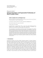
Figure 1: 4-QAM as an example of a continuous channel model.
Signaling points (black circles) and contour lines of a two-
dimensional Gaussian noise distribution with unit variances and
correlation ρ
= 0.8areshown.
1 −ε
1
−δ
0
0
XY
1
1
ε
δ
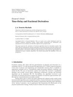
Figure 2: The binary asymmetric channel.
is considered in [4]. Jorswieck and Boche [5]investigatea
similar minimax setup for a single link in a MIMO system
with different types of interference. Further extensions to

vector channels and different kinds of games are considered
(e.g., [6, 7]).
In this paper, we choose the approach that nature
gambles against the transmitter, which aims at conveying
information across the channel in an optimal way. “Nature”
and “channel” are used synonymously to characterize the
antagonist of the transmitter. We consider two models of the
channel which yield comparable results. First, transmission
is considered purely on a symbol basis. Symbols from a
finite set are transmitted and decoded with certain error
probabilities. The model is completely discrete, and strategies
of nature are described by certain channel matrices chosen
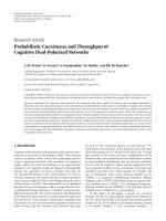
from the set of stochastic matrices. The binary asymmetric
erasure channel as shown in Figure 4 may serve as a typical
example.
On the other hand, continuous channel models are
considered. The strategies of the channel are then given by a
set of densities, each describing the conditional distribution
of received values given a transmitted symbol. The finite
input additive white Gaussian noise channel is a standard
example hereof, and also 4-QAM with correlated noise (e.g.,
as shown in Figure 1)iscoveredbythismodel.
For both models, equilibrium points are sought, where
the strategy of the transmitter consists of selecting the
optimum input distribution against the worst-case behavior
1
1
−δ
0
0

XY
1
1
δ
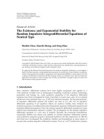
Figure 3: The Z-channel.
1 −ε
1
−δ
00
X
e
Y
1
1
ε
δ
Figure 4: The binary asymmetric erasure channel.
of the channel, vice versa, and both have the same game
value.
The contributions of this paper are as follows. In
Section 2, we demonstrate that mutual information is a
convex function of the channel matrix, or the noise den-
sities, respectively. For discrete channels, transmission is
considered as a game in Section 3. Some typical binary
and n-ary channels are covered by this theory, as shown
in Section 5. It is demonstrated that equilibrium points
exist and the according optimum strategies for both players
are determined. The entropy of mixture distributions is
considered in Section 6, which finally, in Section 7,leadsto
equilibrium points for mixed discrete-continuous channel

strategies.
2. Channel Models and
Mathematical Foundations
Denote the set of stochastic vectors of dimension m by
D
m
=

p = (p
1
, , p
m
) | p
i
≥ 0,
m

i=1
p
i
= 1

. (2)
Each p
∈ D
m
represents a discrete distribution with m
support points. The entropy H of p is defined as
H(p)
=−

m

i=1
p
i
log p
i
. (3)
If p characterizes the distribution of some discrete random
variable X,wesynonymouslywriteH(X)
= H(p). It is
well known that the entropy H is a concave function of
p, and furthermore, even Schur-concave over the set of
distributions D
m
, since it is symmetric (see [8]).
Let random variable X denote the discrete channel input
with symbol set
{x
1
, , x
m
}and distribution p. Accordingly,
random variable Y denotes the output of the channel.
EURASIP Journal on Advances in Signal Processing 3
2.1. Dis crete Output Channels. We first deal with discrete
channels. If the output set consists of n symbols
{y
1
, , y

n
},
then the behavior of the channel is completely characterized
by the (m
×n) channel matrix:
W
= (w
ij
)
1≤i≤m,1≤j≤n
,(4)
consisting of conditional probabilities w
ij
= P(Y = y
j
| X =
x
i
). Matrix W is an element of the set of stochastic (m × n)
matrices, denoted by S
m×n
. Its rows are stochastic vectors,
denoted by w
1
, , w
m
∈ D
n
. The distribution of Y is then
given by the stochastic vector q

= pW.
Mutual information for this channel model reads as
I(X; Y)
= H(Y) −H(Y | X)
= H(pW) −
m

i=1
p
i
H(w
i
)
=
m

i=1
p
i
D(w
i
pW),
(5)
where D(··) denotes the Kulback-Leibler divergence,
D(p
q) =
m

i=1
p

i
log
p
i
q
i
(6)
with p, q
∈ D
m
.
Obviously, mutual information depends on the input
distribution p, controlled by the transmitter, and channel
matrix W, controlled by nature. To emphasize this depen-
dence, we also write I(X; Y)
= I(p; W), The following result
is quoted from [9, Lemma 3.5].
Proposition 1. Mutual information I(p; W) is a concave
function of p
∈ D
m
and a convex function of W ∈ S
m×r
.
The proof relies on the representation in the third line of
(5), convexity of the Kulback-Leibler divergence D(p
q)asa
function of the pair (p, q), and concavity of the entropy H.
The problem of maximizing I(p; W)overp or minimiz-
ing I(p; W)overW subject to convex constraints hence fall

into the class of convex optimization problems.
2.2. General Output Channels. Entropy definition (3) gener-
alizes to densities f of absolutely continuous distributions
with respect to a σ-finite measure μ as
H( f )
=

f (y)log f (y) dμ(y)(7)
(see [10]). Practically relevant cases are the discrete case
(3), where μ is taken as the counting measure, densities
f , with respect to the Lebesgue measure λ
n
on the σ-field
ofBorelsetsover
R
n
, and mixtures hereof. These cases
correspond to discrete, continuous, and mixed discrete-
continuous random variables.
The approach in Section 2.1 carries over to densities of
absolutely continuous distributions with respect to μ, as used
in (7). The channel output Y is randomly distorted by noise,
for symbol i governed by μ-density f
i
. Hence, the distribution
of Y given input X
= x
i
has μ-density
f (y

| x
i
) = f
i
(y), y ∈ R
n
. (8)
The AWGN channel Y
= X + N is a special case hereof
with f
i
(y) = ϕ(y −x
i
). Here, ϕ denotes the Lebesgue density
of a Gaussian distribution N
n
(0, Σ).
Mutual information between channel input and output
as a function of p
= (p
1
, , p
m
)and(f
1
, , f
m
)maybe
written as
I(X; Y)

= I(p;(f
1
, , f
m
))
= H(Y) −H(Y | X)
= H

m

i=1
p
i
f
i

−
m

i=1
p
i
H( f
i
)
=
m

i=1
p

i
D

f
i

m

j=1
p
j
f
j

,
(9)
where D( f
g) =

f log(f/g)dμ denotes the Kullback-
Leibler divergence between μ-densities f and g.
Let F denote the set of all μ-densities. From the convexity
of t log t, t
≥ 0, it is easily concluded that
H

m

i=1
p

i
f
i

is a concave function of p ∈ D
m
. (10)
By applying the log-sum inequality (cf. [9]), we also obtain
αf
1
log
f
1
g
1
+(1− α) f
2
log
f
2
g
2
≥ (αf
1
+(1−α) f
2
)log
αf
1
+(1− α) f

2
αg
1
+(1− α)g
2
,
(11)
pointwise for any pairs of densities ( f
1
, g
1
), (f
2
, g
2
) ∈ F
2
.
Integrating both sides of the aforementioned inequality
shows that
D( f
g) is a convex function of the pair ( f , g) ∈ F
2
. (12)
Applying (10)and(12) to the third and forth lines of rep-
resentation (9), respectively, gives the following proposition.
Proposition 2. Mutual information I(p;(f
1
, , f
m

)) is a
concave function of p
∈ D
m
and a convex function of
( f
1
, , f
m
) ∈ F
m
.
Proposition 2 generalizes its discrete counterpart,
Proposition 1. The latter is obtained from the former by
identifying the rows of W as densities with respect to the
counting measure with support given by the output symbol
set.
In summary, determining the capacity of the channel for
fixed channel noise densities f
1
, , f
m
leads to a concave
optimization problem, namely,
C
= max
p∈D
m
I(p;(f
1

, , f
m
)). (13)
Further, minimizing I(p;(f
1
, , f
m
)) over a convex set of
densities f
1
, , f
m
for some fixed input distribution p ∈ D
m
yields a convex optimization problem.
4 EURASIP Journal on Advances in Signal Processing
3. Discrete Output Channel Games
In what follows, we regard transmission over a channel
as a two-person zero-sum game. A malicious nature is
gambling against the transmitter. If nature is controlling
the channel, the transmitter wants to protect itself against a
worst-case behavior of nature in the sense of maximizing the
capacity of the channel by an appropriate choice of the input
distribution. The question arises whether this type of channel
game has an equilibrium. If the transmitter moves first and
maximizes capacity under the present channel conditions,
is the same game value achieved if nature deteriorates
the channel against the chosen strategy of the transmitter?
Hence, I(X; Y) plays the role of the payoff function.
We will show that for different classes of channels equi-

libria exist. The basis is formed by the following minimax or
saddle point theorem.
Proposition 3. Let T
⊆ S
m×r
be a closed convex subset of
channel matrices. Then the according channel game has an
equilibrium point with value
max
p∈D
m
min
W∈T
I(p; W) = min
W∈T
max
p∈D
m
I(p; W). (14)
The proof is an immediate consequence of von Neu-
mann’s minimax theorem (cf. [11, page 131]). Since D
m
and T are closed and convex, the main premises are
concavity in p and convexity in W,bothpropertiesassured
by Proposition 1.
If T
= S
m×r
, the value of the game is zero. Nature will
make the channel useless by selecting

W
=
⎛
⎜
⎜
⎜
⎜
⎝
w
.
.
.
w
⎞
⎟
⎟
⎟
⎟
⎠
, (15)
with constant rows w yielding I(p; W)
= 0 independent of
the input distribution. Obviously, (15) holds if and only if
input X and output Y are stochastically independent.
We first consider the case that nature plays a singleton
strategy, hence T
={W}, a set consisting of only
one strategy. However, (14) then reduces to determining
max
p∈D

m
I(p; W), the capacity C of the channel for fixed
channel matrix W. In order to characterize nonzero capacity
channels, we use the variational distance between the ith and
jth row of W,definedas
d(w
i
, w
j
) =
r

k=1
|w
ik
−w
jk
|. (16)
The condition
max
1≤i,j≤m
d(w
i
, w
j
) = γ(W) > 0 (17)
on the channel matrix W ensures that the according channel
has nonzero capacity, as demonstrated in the following
proposition.
Proposition 4. If W satisfies (17) for some γ(W) > 0, then

C
= max
p∈D
m
I(p; W) ≥
γ
2
(W)
8ln2
> 0, (18)
where information is measured in nats.
Proof. Let the maximum in (17) be attained at indices i
0
and
j
0
. Further, set p = (1/2)(e
i
0
+ e
j
0
)wheree
i
denotes the ith
unit row vector in
R
m
. The third line in (5) then gives
I(p; W)

=
1
2
D

w
i
0

w
i
0
+ w
j
0
2

+
1
2
D

w
j
0

w
i
0
+ w

j
0
2

.
(19)
Since
D(w
i
w
j
) ≥
1
2ln2
d
2
(w
i
, w
j
) (20)
(see [9, page 58]), and
d

w
i
,
w
i
+ w

j
2

=
1
2
d(w
i
, w
j
), (21)
it follows that
I(p; W)
≥
1
8ln2
d
2
(w
i
0
, w
j
0
) =
γ
2
8ln2
> 0. (22)
In summary, some channel with transition probabilities

W has nonzero capacity if and only if γ(W) > 0. The
same condition turns out important when determining the
capacity of arbitrary discrete channels.
Proposition 5. Let channel matrix W satisfy c ondition (17).
Then C
= max
p∈D
m
I(p; W) is attained at p
∗
= (p
∗
1
, , p
∗
m
)
if and only if
D(w
i
p
∗
W) = ζ (23)
for some ζ>0 and all i with p
∗
i
> 0. Moreover, C =
I(p
∗
; W) = ζ holds.

Proof. Mutual information I(p; W) is a concave function of
p. Hence the KKT conditions (cf., e.g., [12]) are necessary
and sufficient for optimality of some input distribution p.
Using (5), some elementary algebra shows that
∂
∂p
i
I(p; W) = D(w
i
pW) − 1. (24)
The full set of KKT conditions now reads as
p
∈ D
m
,
λ
i
≥ 0, i = 1, , m,
λ
i
p
i
= 0, i = 1, , m,
D(w
i
pW)+λ
i
+ ν = 0, i = 1, , m,
(25)
which shows the assertion.

Proposition 5 has an interesting interpretation. For an
input distribution p
∗
= (p
∗
1
, , p
∗
m
)tobecapacity-
achieving, the Kulback-Leibler distance between the rows
of W and the weighted average with weights p
∗
i
has to
be the same for all i with positive p
∗
i
.Hence,capacity-
achieving distribution p
∗
places the mixture distribution
p
∗
W somehow in the middle of all rows w
∗
i
.
EURASIP Journal on Advances in Signal Processing 5
4. Elementary Channel Models

Discrete binary input channels are considered in this section.
From the according channel games capacity-achieving distri-
butions against worst-case channels are obtained.
4.1. The Binary Asymmetric Channel. As an example, we
consider the binary asymmetric channel with channel
matrix:
W
= W(ε, δ) =
⎛
⎝
1 − εε
δ 1
−δ
⎞
⎠
=
⎛
⎝
w
1
w
2
⎞
⎠
, (26)
with 0 <ε, δ<1 such that condition (17) is satisfied (see
Figure 2). By (23), the capacity-achieving input distribution
p
= (p
0

, p
1
)satisfies
D(w
1
pW) = D(w
2
pW). (27)
This is an equation in the variables p
0
, p
1
which jointly with
the condition p
0
+ p
1
= 1 has the solution
p
∗
0
=
1
1+b
, p
∗
1
=
b
1+b

, (28)
with
b
=
aε −(1 −ε)
δ − a(1 −δ)
, a
= exp

h(δ) −h(ε)
1 − ε −δ

, (29)
and h(ε)
= H(ε,1− ε), the entropy of (ε,1− ε). This result
has been derived by cumbersome methods in the early paper
[13].
Now assume that the strategy set of nature is given by
T
ε,

δ
=

W(ε, δ) | 0 ≤ ε ≤ ε,0≤ δ ≤

δ

, (30)
where 0

≤ ε,

δ<1/2 are given. Hence, error probabilities are
bounded from the worst case by
ε and

δ.
Since I(p; W) is a convex function of W, I(p; W(ε, δ))
is a convex function of the argument (ε, δ)
∈ [0, 1]
2
.The
minimum value 0 is obviously attained whenever ε + δ
= 1.
This shows that I(p; W(ε, δ)) is decreasing in ε
∈ [0, ε]for
fixed δ, and vice versa, is a decreasing function of δ
∈ [0,

δ]
with ε fixed. Accordingly, it holds that
min
W∈T
ε,

δ
I(p; W) = I(p; W(ε,

δ)) (31)
for any p

∈ D
2
. Further,
max
p∈D
2
min
W∈T
ε,

δ
I(p; W) = max
p∈D
2
I

p; W(ε,

δ)

(32)
is attained at p
∗
= (p
∗
0
, p
∗
1
)from(28) with the replacements

ε
= ε and δ =

δ.
Since T
ε,

δ
is a convex set, we obtain from Proposition 3
that a saddle point exists and the value of the game is given
by
max
p∈D
2
min
W∈T
ε,

δ
I(p; W) = min
W∈T
ε,

δ
max
p∈D
2
I(p; W)
= I


p
∗
; W(ε,

δ)

.
(33)
The so-called Z-channel with error probability ε
= 0and
δ
∈ [0, 1] (see Figure 3)isaspecialcasehereof.Wehave
max
p∈D
2
min
δ≤

δ
I(p; W(0, δ)) = max
p∈D
2
I(p; W(0,

δ))
= I(p
∗
; W(0,

δ)).

(34)
After some algebra, from (28)
p
∗
0
= 1 − p
∗
1
, p
∗
1
=
1/(1 −

δ)
1 − 2
h(

δ)/(1−

δ)
(35)
is obtained with capacity
I

p
∗
; W(0,

δ)


=
log
2

1+2
−h(

δ)/(1−

δ)

, (36)
where information is measured in bits (cf. [14, Example
9.11]).
4.2. The Binary Asymmetric Erasure Channel. The binary
asymme tric erasure channel (BEC) with bit error probabilities
ε, δ
∈ [0, 1], and channel matrix
W
= W(ε, δ) =
⎛
⎝
1 − εε 0
0 δ 1
−δ
⎞
⎠
(37)
is depicted in Figure 4.

According to Proposition 4, this channel has zero capac-
ity if and only if ε
= δ = 1. Excluding this case, by
Proposition 5, the capacity-achieving distribution p
∗
=
(p
∗
0
, p
∗
1
), p
∗
0
+ p
∗
1
= 1 is given by the solution of
(1
−ε)log
1
−ε
p
0
(1 − ε)
+ ε log
ε
p
0

ε + p
1
δ
= δ log
δ
p
0
ε + p
1
δ
+(1
−δ)log
1
−δ
p
0
(1 − δ)
.
(38)
Substituting x
= p
0
/p
1
,(38) reads equivalently as
ε logε
−δ logδ = (1 − δ)log(δ + εx) −(1 −ε)log

ε +
δ

x

.
(39)
By differentiating with respect to x, it is easy to see that the
right-hand side is monotonically increasing such that exactly
one solution p
∗
= (p
∗
1
, p
∗
2
) exists, which can be numerically
computed.
If ε
= δ, the solution is given by p
∗
0
= p
∗
1
= 1/2, as easily
verified from (38).
Resembling the arguments used for the binary asymmet-
ric channel and adopting the notation, we see that
min
W∈T
ε,


δ
I(p; W) = I

p; W(ε,

δ)

(40)
for any p
∈ D
2
. Further,
max
p∈D
2
min
W∈T
ε,

δ
I(p; W) = max
p∈D
2
I

p; W(ε,

δ)


(41)
6 EURASIP Journal on Advances in Signal Processing
is attained at p
∗
= (p
∗
0
, p
∗
1
), the solution of (38)withε
substituted by
ε and δ by

δ. Finally, the game value amounts
to
max
p∈D
2
min
W∈T
ε,

δ
I(p; W) = min
W∈T
ε,

δ
max

p∈D
2
I(p; W)
= I

p
∗
; W(ε,

δ)

.
(42)
If δ
= ε ≤ ε, the result is
I

p
∗
; W(ε,

δ)

=
1 − ε, (43)
and the equilibrium strategies are p
∗
0
= p
∗

1
= 1/2 for the
transmitter and ε
= δ = ε for nature (cf. [15, Example 8.5]).
5. The n-Ary Symmetric Channel
Consider the n-ary symmetric channel with symbol set
{0, 1, , n −1} and channel matrix
W(ε)
=
⎛
⎜
⎜
⎜
⎜
⎜
⎜
⎜
⎝
ε
0
ε
1
··· ε
n−1
ε
n−1
ε
0
··· ε
n−2

.
.
.
.
.
.
.
.
.
.
.
.
ε
1
ε
2
··· ε
0
⎞
⎟
⎟
⎟
⎟
⎟
⎟
⎟
⎠
(44)
by cyclically shifting some error vector ε
= (ε

0
, ε
1
, , ε
n−1
) ∈
D
n
.LetE ⊆ D
n
denote the set of strategies that nature can
choose the channel state from by selecting some ε
∈ E .
If E
= D
n
, the value of the game is zero. As mentioned
earlier, nature will cripple the channel by selecting
ε
= ε
u
=

1
n
, ,
1
n

, (45)

yielding I(X; Y)
= 0 independent of the input distribution.
Note that ε
u
is the unique minimum element with respect
to majorization, that is, ε
u
≺ ε for all ε ∈ D
n
.Webriefly
recall the corresponding definitions (see [8]). Let p
[i]
and
q
[i]
denote the components of p and q in decreasing order,
respectively. Distribution p
∈ S is said to be majorized by
q
∈ S,insymbolsp ≺ q,if

k
i
=1
p
[i]
≤

k
i

=1
q
[i]
for all
k
= 1, ,m.
Hence, to avoid trivial cases, the set of strategies for
nature has to be separated from this worst case.
5.1. Separation by Schur Ordering. We first investigate the set
E
ε
={ε = (ε
0
, , ε
n−1
) ∈ D
n
|

ε ≺ ε, ε
π(0)
≤···≤ε
π(n−1)
}
(46)
for some fixed
ε
/
=ε
u

and permutation π. This means that
the error probabilities are at least spread out, or separated
from uniformity as
ε, with error probabilities increasing in
the fixed order determined by π.
Since E
ε
is convex and closed, the set of corresponding
matrices
T
ε
={W(ε) | ε ∈ E
ε
} (47)
is convex and closed as well.
Proposition 3 ensures the existence of an equilibrium
point:
max
p∈D
n
min
W∈T
ε
I(p; W) = min
W∈T
ε
max
p∈D
n
I(p; W). (48)

To determine the value v of the game, we first consider
max
p∈D
n
I(p; W(ε)) for some fixed ε ∈ E
ε
.From(5), it
follows that the maximum is attained at input distribution
p
= (1/n, ,1/n)withvalue
max
p∈D
n
I(p; W(ε)) = log n −H(ε). (49)
As the entropy is Schur concave, min
ε∈E
ε
(log n − H(ε)) is
attained at
ε such that the value of the game is obtained as
min
W∈T
ε
max
p∈D
n
I(p; W) = log n −H(ε) (50)
with according equilibrium strategies p
= (1/n, ,1/n)and
the components of ε equal to those of

ε rearranged according
to π.
5.2. Directional Separation. In what follows, we consider
channel states separated from the worst-case ε
u
into the
direction of some prespecified
ε ∈ D
n
, ε
/
=ε
u
.Thissetof
strategies is formally described as
E
α,ε
={ε = (1 −α)ε
u
+ αε | α ≤ α ≤ 1} (51)
for some given α>0. It is obviously convex and closed. The
set of corresponding channel matrices
T
α,ε
={W(ε) | ε ∈ E
α,ε
} (52)
is also closed and convex such that an equilibrium exists by
Proposition 3. It remains to determine the game value.
Since I(p; W) is a convex function of W, hence decreasing

in α
∈ [α,1):
min
W∈T
α,ε
I(p; W) (53)
is attained at W(ε
α
)withε
α
= (1 − α)ε
0
+ αε.From
representation (5), it can be easily seen that
max
p∈D
n
min
W∈T
α,ε
I(p; W) (54)
is attained at p
= (1/n, ,1/n).
Vice versa, from (5), it follows that for any W
= W(ε),
max
p∈D
n
I(p; W(ε)) = log n −H(ε) (55)
is attained at p

= (1/n, ,1/n)foranyε ∈ E
α,ε
.By
monotonicity in α
∈ [α, 1), it holds that
min
W∈T
α,ε
max
p∈D
n
I(p; W) = log n −H(ε
α
), (56)
which determines the game value. The equilibrium strategies
are the uniform distribution for the transmitter and the
extreme error vector ε
α
for nature.
EURASIP Journal on Advances in Signal Processing 7
The n-ary symmetric channel with error probabilities

1 − δ,
δ
n − 1
, ,
δ
n − 1

(57)

is a special case of the aforementioned by identifying
ε =
(1, 0, ,0)andα = 1 −(n/(n − 1))δ.
The binary symmetric channel (BSC) with error proba-
bility 0 <δ<1/2 is obtained by setting n
= 2, ε = (1, 0) and
α
= 1 −2δ.
6. Entropy of Mixture Distributions
Let U be an absolutely continuous random variable with
density g(y) with respect to to the Lebesgue measure λ
n
,
and let random variable V have a discrete distribution with
discrete density h(y)
= p
i
,ify = x
i
, i = 1, , m,andh(y) =
0 otherwise, p
i
≥ 0,

m
i=1
p
i
= 1. Furthermore, assume that B
is Bernoulli distributed with parameter α,0

≤ α ≤ 1, hence
P(B
= 1) = α, P(B = 0) = 1 − α. Further, let U, V, B be
stochastically independent, then
W
= BU +(1− B)V (58)
has density
f (y)
= αg(y)+(1− α)h(y) (59)
with respect to the measure μ
= λ
n
+ χ,whereχ denotes
the counting measure with support
{x
1
, , x
m
}. According
to [10], the entropy of W is defined as
H(W) =−

f (y)log f (y) dμ(y). (60)
It easily follows (see [16]) that
H(W)
=−α

g(y)logg(y) dy −α logα
−(1 −α)
m


i=1
p
i
log p
i
−(1 −α)log(1− α)
= H(B)+αH(U)+(1−α)H(V).
(61)
The following proposition will be useful when investi-
gating equilibria of channel games with continuous noise
densities.
Proposition 6. Let p
= (p
1
, , p
m
) denote some stochastic
vector, and g
1
, , g
m
be densities with respect to some measure
μ.Itholdsthat
H

m

i=1
p

i
g
i

−
m

i=1
p
i
H(g
i
) ≤ H(p). (62)
The proof is provided by the following chain of equalities
and inequalities. The argument y of g
i
is omitted for reasons
of brevity:
−



i
p
i
g
i

log



j
p
j
g
j

dμ +

i
p
i

g
i
log g
i
dμ
=−

i
p
i

g
i

log



j
p
j
g
j

−
log g
i

dμ
=

i
p
i

g
i
log
g
i

j
p
j
g
j
dμ
≤


i
p
i

g
i
log
g
i
p
i
g
i
dμ
=−

i
p
i
log p
i
= H(p).
(63)
7. A Mixed Discrete-Continuous Channel Game
Let g
1
, , g
m
be given λ

n
-densities. Distribution p
∗
=
(p
∗
1
, , p
∗
m
) achieves capacity, that is, maximizes mutual
information if and only if I(X; Y) is maximized by p
∗
in the
set of all stochastic vectors. By representation (9), we need to
solve
maximize

−


m

i=1
p
i
g
i
(y)


log

m

i=1
p
i
g
i
(y)

dy
+
m

i=1
p
i

g
i
(y)logg
i
(y) dy

subject to p
i
≥ 0, i = 1, , m,
m


i=1
p
i
= 1.
(64)
The aforementioned is a convex problem since by
Proposition 2, the objective function is concave and the
constraint set is convex. The Lagrangian is given by
L(p, μ, ν)
=−


m

i=1
p
i
g
i
(y)

log

m

i=1
p
i
g
i

(y)

dy
−
m

i=1
p
i

g
i
(y)logg
i
(y) dy
+
m

i=1
μ
i
p
i
+ ν

m

i=1
p
i

−1

,
(65)
with the notation μ
= (μ
1
, , μ
m
). The optimality condi-
tions are (cf. [12, Chapter 5.5.3])
∂L(p, μ, ν)
∂p
i
= 0,
p
i
, μ
i
≥ 0,
μ
i
p
i
= 0,
(66)
8 EURASIP Journal on Advances in Signal Processing
for all i
= 1, ,m. Partial derivatives of the Lagrangian with
respect to p

i
are easily obtained as
∂L(p, μ, ν)
∂p
i
=−(loge) −

g
i
(y)log

m

j=1
p
j
g
j
(y)

dy
+

g
i
(y)logg
i
(y) dy + μ
i
+ ν,

(67)
for i
= 1, ,m.Hence(66) leads to the conditions p
i
= 0or

g
i
(y)

log g
i
(y) − log

m

j=1
p
j
g
j
(y)

dy = log e − ν, (68)
for all i
= 1, , m. In summary, we have demonstrated the
following result.
Proposition 7. Let g
1
, , g

m
be Lebesgue λ
n
-densities. Input
distribution p
∗
is capacity-achieving if and only if
D

g
i

m

j=1
p
∗
j
g
j

=
ζ, (69)
for some ζ>0,foralli such that p
∗
i
> 0.Furthermore,ifH(g
i
)
is independent of i, then p

∗
is capacity-achieving if and only if

g
i
(y)log

m

j=1
p
∗
j
g
j
(y)

dy = ξ (70)
for some ξ
∈ R,foralli such that p
∗
i
> 0.
Now, assume that the strategy set of the channel consists
of the densities
F
=

f
(α)

1
(y), , f
(α)
m
(y)

|
f
(α)
i
(y) = αg
i
(y)+(1− α)h
i
(y), 0 ≤ α ≤ 1

,
(71)
where g
i
are densities with respect to λ
n
and h
i
represents the
singleton distribution with support point x
i
. f
(α)
i

are hence
densities with respect to the measure λ
n
+ χ.
F represents a closed convex line segment in the
space of all densities, reaching from error distribution
(g
1
, , g
m
)atα = 1 to the error-free singleton distribution
(h
1
, , h
m
)atα = 0. The strategy set is analogous to the
m-ary discrete output case with directional separation in
Section 5.2.InFigure 5, the mixture of a standard Gaussian
and the singleton distribution in 0 is depicted for α
∈
{
0.0, 0.25, 0.5, 0.75,1.0}. Densities are with respect to the
measure λ
1
+ χ(0).
Intuitively, it seems to be clear that the channel would
choose the extreme value α
= 1 as the worst case to jam the
transmitter. A precise proof of this fact, however, is amazingly
complicated.

α
1
0.75
0.5
0.25
Figure 5: Mixture density of a standard Gaussian and a singleton
distribution in 0. Densities are with respect to the measure λ
1
+ χ.
By (61), mutual information is given as
I(X; Y)
= I

p;

f
(α)
1
, , f
(α)
m

=
H

m

i=1
p
i

f
(α)
i

−
m

i=1
p
i
H

f
(α)
i

=
H

α
m

i=1
p
i
g
i
+(1− α)
m


i=1
p
i
h
i

−
m

i=1
p
i
H(αg
i
+(1− α)h
i
)
= H(α,1− α)+αH

m

i=1
p
i
g
i

+(1−α)H(p)
−
m


i=1
p
i
(H(α,1− α)+αH(g
i
))
= α

H

m

i=1
p
i
g
i

−
m

i=1
p
i
H(g
i
) − H(p)

+ H(p).

(72)
Since by Proposition 6, the term in curly brackets in the
last line of (72) is nonpositive, for any p, the minimum of
I(p;(f
(α)
1
, , f
(α)
m
)) over α ∈ [0,1]isattainedatα = 1with
value
H

m

i=1
p
i
g
i

−
m

i=1
p
i
H(g
i
) =

m

i=1
p
i
D

g
i

m

j=1
p
j
g
j

. (73)
From Proposition 7, it follows that the right-hand side is
maximized at p
∗
∈ D
m
whenever
D

g
i
|

m

j=1
p
∗
j
g
j

=
ζ (74)
for all i with p
∗
i
> 0.
EURASIP Journal on Advances in Signal Processing 9
In summary, the channel game has an equilibrium point
max
p∈D
m
min
( f
(α)
1
, , f
(α)
m
)∈F
I


p;

f
(α)
1
, , f
(α)
m

=
min
( f
(α)
1
, , f
(α)
m
)∈F
max
p∈D
m
I

p;

f
(α)
1
, , f
(α)

m

.
(75)
The equilibrium strategy for the channel is given by α
= 1.
The optimum strategy p
∗
for the transmitter is characterized
by (74). For certain error distributions g
j
this condition can
be explicitly evaluated (see [17]).
8. Conclusions
We have investigated Nash equilibria for a two-person zero-
sum game where the channel gambles against the transmitter.
The transmitter strategy set consists of all input distributions
over a finite symbol set, while the channel strategy sets are
formed by certain convex subsets of channel matrices or
noise distributions, respectively. Mutual information is used
as payoff function.
Basically, it is assumed that a malicious nature is con-
trolling the channel such that equilibria are achieved when
the transmitter plays the capacity-achieving distribution
against worst-case attributes of the channel. In practice,
however, a wireless channel is only partially controlled by
nature, for example, by shadowing and attenuation effects,
further, diffraction and reflection. A major contribution to
the channel properties, however, is made by interference
from other users. It will be a subject of future research to

investigate how these effects may be combined in a single
strategy set of the channel. The question arises if equilibria
for the game “one transmitter against a group of others plus
random effects from nature” still exist.
Acknowledgments
Part of the material in this paper was presented at IEEE
ISIT 2008, Toronto. This work was partially supported by the
UMIC Research Center at RWTH Aachen University.
References
[1] A. Leshem and E. Zehavi, “Bargaining over the interference
channel,” in Proceedings of IEEE International Symposium on
Information Theory (ISIT ’06), pp. 2225–2229, Seattle, Wash,
USA, July 2006.
[2] S. Mathur, L. Sankaranarayanan, and N. B. Mandayam,
“Coalitional games in Gaussian interference channels,” in
Proceedings of IEEE International Symposium on Information
Theory (ISIT ’06), pp. 2210–2214, Seattle, Wash, USA, July
2006.
[3] J. M. Borden, D. M. Mason, and R. J. McEliece, “Some
information theoretic saddlepoints,” SIAM Journal on Control
and Optimization, vol. 23, no. 1, pp. 129–143, 1985.
[4] S. N. Diggavi and T. M. Cover, “The worst additive noise under
a covariance constraint,” IEEE Transactions on Information
Theory, vol. 47, no. 7, pp. 3072–3081, 2001.
[5] E. A. Jorswieck and H. Boche, “Performance analysis of
capacity of MIMO systems under multiuser interference based
on worst-case noise behavior,” EURASIP Journal on Wireless
Communications and Networking, vol. 2004, no. 2, pp. 273–
285, 2004.
[6]D.P.Palomar,J.M.Cioffi, and M. A. Lagunas, “Uni-

form power allocation in MIMO channels: a game-theoretic
approach,” IEEE Transactions on Information Theory, vol. 49,
no. 7, pp. 1707–1727, 2003.
[7] A. Feiten and R. Mathar, “Minimax problems and directional
derivatives for MIMO channels,” in Proceedings of the 63rd
IEEE Vehicular Technology Conference (VTC ’06), vol. 5, pp.
2231–2235, Melbourne, Australia, May 2006.
[8] A.W.MarshallandI.Olkin,Inequalities: Theory of Majoriza-
tion and Its Applications, Academic Press, New York, NY, USA,
1979.
[9] I. Csiszar and J. K
¨
orner, Information Theory: Coding Theorems
for Discrete Memoryless Systems, Academic Press, London, UK,
1981.
[10] M. Pinsker, Information and Information Stability of Random
Variables and Processes, Holden-Day, San Francisco, Calif,
USA, 1964.
[11] A. W. Roberts and D. E. Varberg, Convex Functions,Academic
Press, New York, NY, USA, 1973.
[12] S. Boyd and L. Vandenberghe, Convex Optimization,Cam-
bridge University Press, New York, NY, USA, 2004.
[13] R. A. Silverman, “On binary channels and their cascades,” IRE
Transactions on Information Theory, vol. 1, no. 3, pp. 19–27,
1955.
[14] D. J. C. MacKay, Information Theory, Inference, and Learning
Theory, Cambridge University Press, Cambridge, UK, 2003.
[15] R. W. Yeung, A First Course in Information Theory,Kluwer
Academic Publishers/Plenum Press, New York, NY, USA, 1st
edition, 2002.

[16] D. N. Politis, “Maximum entropy modelling of mixture
distributions,” Kybernetes, vol. 23, no. 1, pp. 49–54, 1994.
[17] A. Feiten and R. Mathar, “Capacity-achieving discrete sig-
naling over additive noise channels,” in Proceedings of IEEE
International Conference on Communications (ICC ’07),pp.
5401–5405, Glasgow, UK, June 2007.