Báo cáo hóa học: " Research Article Inference of Gene Regulatory Networks Based on a Universal Minimum Description Length" pot

Hindawi Publishing Corporation
EURASIP Journal on Bioinformatics and Systems Biology
Volume 2008, Article ID 482090, 11 pages
doi:10.1155/2008/482090
Research Article
Inference of Gene Regulatory Networks Based on
a Universal Minimum Description Length
John Dougherty, Ioan Tabus, and Jaakko Astola
Institute of Signal Processing, Tampere University of Technology, P.O. Box 553, 33101 Tampere, Finland
Correspondence should be addressed to John Dougherty, john.dougherty@tut.fi
Received 24 August 2007; Accepted 11 January 2008
Recommended by Aniruddha Datta
The Boolean network paradigm is a simple and effective way to interpret genomic systems, but discovering the structure of these
networks remains a difficult task. The minimum description length (MDL) principle has already been used for inferring genetic
regulatory networks from time-series expression data and has proven useful for recovering the directed connections in Boolean
networks. However, the existing method uses an ad hoc measure of description length that necessitates a tuning parameter for
artificially balancing the model and error costs and, as a result, directly conflicts with the MDL principle’s implied universality. In
order to surpass this difficulty, we propose a novel MDL-based method in which the description length is a theoretical measure
derived from a universal normalized maximum likelihood model. The search space is reduced by applying an implementable
analogue of Kolmogorov’s structure function. The performance of the proposed method is demonstrated on random synthetic
networks, for which it is shown to improve upon previously published network inference algorithms with respect to both speed
and accuracy. Finally, it is applied to time-series Drosophila gene expression measurements.
Copyright © 2008 John Dougherty et al. This is an open access article distributed under the Creative Commons Attribution
License, which permits unrestricted use, distribution, and reproduction in any medium, provided the original work is properly
cited.
1. Introduction
The modeling of gene regulatory networks is a major focus of
systems biology because, depending on the type of modeling,
the networks can be used to model interdependencies
between genes, to study the dynamics of the underlying
genetic regulation, and to provide a basis for the derivation

of optimal intervention strategies. In particular, Bayesian
networks [1, 2] and dynamic Bayesian networks [3, 4]
provide models to elucidate dependency relations; functional
networks, such as Boolean networks [5] and probabilistic
Boolean networks [6], provide the means to characterize
steady-state behavior. All of these models are closely related
[7].
When inferring a network from data, regardless of the
type of network being considered, we are ultimately faced
with the difficulty of finding the network configuration
that best agrees with the data in question. Inference starts
with some framework assumed to be sufficiently complex
to capture a set of desired relations and sufficiently simple
to be satisfactorily inferred from the data at hand. Many
methods have been proposed, for instance, in the design of
Bayesian networks [8] and probabilistic Boolean networks
[9]. Here we are concerned with Boolean networks, for which
a number of methods have been proposed [10–14]. Among
the first information-based design algorithms is the Reveal
algorithm, which utilizes mutual information to design
Boolean networks from time-course data [11]. Information-
theoretic design algorithms have also been proposed for non-
time-course data [15, 16].
Here we take an information-theoretic approach based
on the minimum description length (MDL) principle [17].
The MDL principle states that, given a set of data and
class of models, one should choose the model providing
the shortest encoding of the data. The coding amounts to
storing both the network parameters and any deviations
of the data from the model, a breakdown that strikes a

balance between network precision and complexity. From
the perspective of inference, the MDL principle represents
a form of complexity regularization, where the intent is
generally to measure the goodness of fit as a function of
some error and some measure of complexity so as not
2 EURASIP Journal on Bioinformatics and Systems Biology
to overfit the data, the latter being a critical issue when
inferring gene networks from limited data. Basically, in
addition to choosing an appropriate type, one wishes to
select a model most suited for the amount of data. In essence,
the MDL principle balances error (deviation from the data)
and model complexity by using a cost function consisting
of a sum of entropies, one relative to encoding the error
and the other relative to encoding the model description
[18]. The situation is analogous to that of structural risk
minimization in pattern recognition, where the cost function
for the classifier is a sum of the resubstitution error of
the empirical-error-rule classifier and a function of the VC
dimension of the model family [19]. The resubstitution error
directly measures the deviation of the model from the data
and the VC dimension term penalizes complex models. The
difficulties are that one must determine a function of the VC
dimension and that the VC dimension is often unknown, so
that some approximation, say a bound, must be used. The
MDL principle was among the first methods used for gene
expression prediction using microarray data [20].
Recently, a time-course-data algorithm, henceforth
referred to as Network MDL [10], was proposed based on the
MDL principle. The Network MDL algorithm often yields
good results, but it does so with an ad hoc coding scheme

that requires a user-specified tuning parameter. We will avoid
this drawback by achieving a codelength via a normalized
maximum likelihood model. In addition, we will improve
upon Network MDL’s efficiency by applying an analogue of
Kolmogorov’s structure function [21].
2. Background
2.1. Boolean Networks
Using notation modified from Akutsu et al. [12], a Boolean
network is a directed graph G(V, Λ, F) defined by a set
V
={v
i
}
g
i
=1
of g binary-valued nodes representing genes,
a collection of structure parameters Λ
={λ
i
}
g
i
=1
indicating
their regulatory sets (predecessor genes), and the Boolean
functions F
={f
i
}

g
i
=1
regulating their behavior. Specifically,
each structure parameter λ
i
={i
1
, , i
k
i
} is the collection of
indices i
1
<i
2
< ··· <i
k
i
associated with v
i
’s regulatory
nodes. The number k
i
of regulatory nodes for node v
i
is
referred to as the indegree of v
i
. We assume that the nodes

are observed over n + 1 equally spaced time points, and we
write y
i,t
∈ B ={0,1} to denote the values of node i for
t
= 0, 1, , n. The value of node v
i
progresses according to
y
i,t
= f
i

y
i
1
,t−1
, y
i
2
,t−1
, , y
i
k
i
,t−1

(1)
for t
= 1, , n. Such synchronous updating is perhaps

unrealistic in biological systems, but it provides a frame-
work with more easily tractable models and has proven
useful in the present context [22]. For ease of notation,
we define the inputs of f
i
as the column vector x
i,t
=
[y
i
1
,t−1
, y
i
2
,t−1
, , y
i
k
i
,t−1
]

, allowing us to rewrite (1)as
y
i,t
= f
i

x

i,t

, t = 1, , n. (2)
The fundamental question we face is the estimation of Λ
and F. Note that Λ is usually not included as a parameter
of G because it can be absorbed into F,butwechooseto
write it separately because, under the model we will specify,
Λ completely dictates F, making our interest reside primarily
in the structure parameter set Λ.
As written, (2) provides us with a completely deter-
ministic network, but this is generally considered to be an
inadequate description. Measurement error is inescapable in
virtually any experimental setting, and, even if one could
obtain noiseless data, biological systems are constantly under
the influence of external factors that might not even be
identifiable, let alone measurable [6]. Therefore, we consider
it incumbent to relocate our model of the network mecha-
nisms into a probabilistic framework. By incorporating this
philosophy and switching to matrix notation, (2)becomes
Y
i
= f
i

X
i

⊕
ε
i

∈ B
n
,(3)
where
⊕ denotes modulo 2 sum, f
i
acts independently on
each column of X
i
= [x
i,1
, , x
i,n
], and ε
i
is a vector of
independent Bernoulli random variables with P(ε
i,t
= 1) =
θ
i
∈ [0, 1]. We further assume that the errors for different
nodes are independent. We allow θ
i
to depend on i because it
can be interpreted as the probability that node i disobeys the
network rules, and we consider it natural for different nodes
to have varying propensities for misbehaving.
Returning to our overall objective, we observe that λ
i

and
f
i
can be estimated separately for each gene. This is possible
because, for each evaluation of f
i
, X
i
is regarded as fixed and
known. Even if a network was constructed so that a gene was
entirely self-regulatory, that is, λ
i
={i}, the random vector
Y
i
is observed sequentially so that any random variable Y
i,t
within it is observed and then considered as a fixed value
x
i,t+1
before being used to obtain Y
i,t+1
. Therefore, despite
the obvious dependencies that would exist for networks
containing configurations such as feedback loops and nodes
appearing in multiple predecessor sets, the given model
stipulates independence between all random variables. Thus,
we restrict ourselves to estimating the parameters for one
node and rewrite (3)as
Y

= f (X) ⊕ε,(4)
which we recognize as multivariate Boolean regression. Note
that θ
i
and k
i
now become θ and k,respectively.
We finalize the specification of our model by extending
the parameter space for the error rates by replacing θ with
Θ
={θ
l
}
2
k
−1
l
=0
,whereeachθ
l
corresponds to one of the 2
k
possible values of x
t
. This allows the degree of reliability of
the network function to vary based upon the state of a gene’s
predecessors. Note that 2
k
is only an upper bound on the
numberoferrorratesbecausewewillnotnecessarilyobserve

all 2
k
possible regressor values. This model is specified by the
predecessor genes composing X
= [x
1
, , x
n
], the function
f , and the error rates in Θ. Thus, adopting notation from
Tabus et al. [23], we refer to the collection of all possible
parameter settings as the model class M(Θ, λ, f ).
2.2. The MDL Principle
Given the model formulation, we use the MDL principle
as our metric for assessing the quality of the parameter
EURASIP Journal on Bioinformatics and Systems Biology 3
Table 1: Probability table for “OR” function with θ = 0.2.
(x
1
, x
2
) P(Y = 0) P(Y = 1)
(0, 0) 0.8 0.2
(0, 1) 0.2 0.8
(1, 0) 0.2 0.8
(1, 1) 0.2 0.8
estimates. As stated in Section 1, the MDL principle dictates
that, given a dataset and some class of possible models, one
should choose the model providing the shortest possible
encoding of the data. In our case, the MDL principle is

applied for selecting each node’s predecessors. However,
as we have noted, this technique is inherently problematic
because no unique manner of codelength evaluation is
specified by the principle. Letting e
t
= 1 when the node in
question is predicted incorrectly and 0 otherwise, basic cod-
ing theory gives us a residual codelength of
−

n
t
=1
log
2
P(ε
t
=
e
t
), but the cost of storing the model parameters has no such
standard. Thus, we can technically choose any applicable
encoding scheme we like, an allowance that inevitably gives
rise to infinitely many model codelengths and, as a result, no
unique MDL-based solution.
As an example, we refer to the encoding method used
in Network MDL, in which the network is stored via
probability tables such as Table 1 . In this procedure, the
model codelength is calculated as the cost of specifying the
two predecessor genes plus the cost of storing the probability

table. Letting d
i
and d
f
denote the number of bits needed
to encode integers and subunitary floating point numbers,
respectively, the model codelength is 2d
i
+4d
f
. Note that we
only need 4 of the probabilities since each row in the table
adds to 1. This is one of many perfectly reasonable coding
schemes, but we present another method that corresponds
to our model class and yields a shorter codelength. Also, to
demonstrate the risk of using the MDL principle with ad hoc
encodings, we compare results obtained by using these two
schemes in a short artificial example. Observe that Tabl e 1
corresponds to M(Θ, λ, f )witheachθ
l
= 0.2. First, we
encode f as the 4 bits 0111 because, providing all predecessor
combinations are lexographically sorted, those are the values
that Y will be with probability 1
− θ. Assuming we select f
to minimize the error rates, we can also assume that θ
l
∈
[0, 0.5]. Since d
f

bits are sufficient to encode any decimal less
than 1, we really only need d
f
/2bitstostoreeachθ
l
, yielding
a model cost of 2d
i
+2d
f
+4.
To show the effect of the encoding scheme we generated
one hundred 6-gene networks, each of which was observed
over 50 time points. Λ and F were fixed so that one gene
would behave according to Ta ble 1 . The MDL principle was
applied for both of the encoding schemes to determine the
predecessors of that gene. The results are displayed in Table 2 .
We find that the two encoding methods can give different
structure estimates because the shorter model codelength
allows for a greater number of predecessors. Zhao et al.
compensate for this nonuniqueness by adjusting the model
codelength with a weight parameter, but, while necessary
for ad hoc encodings such as the ones discussed so far,
Table 2: Effect of ad hoc encoding schemes on structure inference.
Results are reported as percentages. “Fair” and “Poor” indicate
missing one and both of the two predecessors, respectively.
Encoding method
Model performance Network MDL M(Θ, λ, f )
Correct 0.03 0.08
Fair 0.12 0.17

Poor 0.85 0.75
the presence of such tuning parameters is undesirable
when compared with a more theoretically based method.
Moreover, the MDL principle’s notion of “the shortest
possible codelength” implies a degree of generality that is
violated if we rely upon a user-defined value.
2.3. Normalized Maximum Likelihood
One alternative that alleviates these drawbacks is to measure
codelength based on universal models. In this approach,
we depart from two part description lengths and their ad
hoc parameters by evaluating costs using a framework that
incorporates distributions over the entire model class. The
fundamental idea for such a model is that, assuming a
specific model class, we should choose parameters that max-
imize the probability of the data [21]. Two such models are
the mixture universal model and the normalized maximum
likelihood (NML) model, the latter of which will command
our attention. For M(Θ, λ, f )withafixedλ, the NML
model is introduced by the standard likelihood optimization
problem max
Θ
log P(y; Θ, λ, f ). The solution is obtained for
Θ
=

Θ, the maximum likelihood estimate (MLE), but cannot
be used as a model because P(y;

Θ, λ, f ) does not integrate
to unity. Thus, we will use the distribution q(y) such that

its ideal codelength
−log
2
q(y) is as close as possible to the
codelength
−log
2
P(y;

Θ, λ, f ). This suggests that we should
minimize the difference between using q(y)inplaceof
P(y;

Θ, λ, f ) for the worst case y. The resulting optimization
problem,
min
q
max
y
log
2
P(y;

Θ, λ, f )
q(y)
,(5)
is solved by the NML density function, defined as P(y;

Θ, λ,
f ) divided by the normalizing constant


y∈B
n
P(y;

Θ, λ, f ).
Tabus et al. [23] provide the derivations of this NML
distribution; the following is a brief outline of the major
steps.
Given a realization y of the random variable Y,wehave
residuals
e
= y ⊕ f (X). (6)
Recall that the Bernoulli distribution is defined by
P(ε
= e) = θ
e

1 − θ

1−e
, e ∈ B. (7)
4 EURASIP Journal on Bioinformatics and Systems Biology
Letting b
l
denote the k-bit binary representation of integer l,
combine (6)and(7) to define the probability P

y
t

; f , b
l
, θ
l

as
P

Y
t
= y
t
; x
t
= b
l

=
θ
y
t
⊕f (b
l
)
l

1 − θ
l

1−y

t
⊕f (b
l
)
. (8)
This representation allows us to formally write our model
class as
M(Θ, λ, f )
=

P

y
t
; f , b
l
, θ
l

=
θ
y
t
⊕f (b
l
)
l

1 − θ
l


1−y
t
⊕f (b
l
)

.
(9)
2.3.1. NML Model for M(Θ, λ, f )
Consider any y ∈ B
n
and fixed λ.Letm
l
denote the number
of times each unique regressor vector b
l
∈ B
k
occurs in X,
and let m
l
1
count the number of times b
l
is associated with
a unitary response. As pointed out by Tabus et al. [23], the
MLE for this model is not unique. The network could have
f (b
l

) = 0, in which case

θ
l
= m
l
1
/m
l
,or f (b
l
) = 1, giving

θ
l
= 1 −m
l
1
/m
l
. Either way, the NML model is given by

P(y) =
P

y; λ,

f , X,

Θ



l:b
l
∈X
C
m
l
, (10)
where
P

y; λ,

f , X,

Θ

=

l:b
l
∈X

m
l
1
m
l


m
l
1

1 −
m
l
1
m
l

m
l
−m
l
1
, (11)
C
m
l
=
m
l

i=0

m
l
i


i
m
l

i

1 −
i
m
l

m
l
−i
. (12)
Of course, this means that our model does not explicitly
estimate f . However, considering that Θ represents error
rates, the obvious choice is to minimize each

θ
l
by taking

f (b
l
) = 0 whenever m
l
1
<m
l

− m
l
1
, and 1 otherwise. In
the event that

θ
l
= 1/2, we set

f (b
l
) = 0 if the portion of
y corresponding to b
l
is less than m
l
/2 in binary. Assuming
independent errors, this removes any bias that would result
from favoring a particular value for

f (b
l
) when

θ
l
= 1/2.
This effectively reduces the parameter space for each θ
l

from
[0, 1] to [0, 1/2] which, in turn, affects

P(y) by halving every
C
m
l
. However, we will later show that the algorithm does not
change whether or not we actually specify

f ,andweoptnot
to do so.
Also note that computing C
m
l
exactly may not be
feasible. For example, Matlab loses precision for the binomial
coefficient (
m
l
i
) when m
l
> 53. In these cases, we use
C
m
l
≈

πm

l
2
+
2
3
+

1
24


2π
m
l
, (13)
an approximation given in [24]. For the sake of efficiency,
we compute every C
m
l
prior to learning the network so that
calculating the denominator of (10) takes at most min(n,2
k
)
operations.
2.3.2. Stochastic Complexity
We take as the measure of a selected model’s total codelength
the stochastic complexity of the data, which is defined as
the negative base 2 logarithm of the NML density function
[21]. As was already the case for the residual codelength, the
stochastic complexity is a theoretical codelength and will not

necessarily be obtainable in practice, but it is precisely this
theoretical basis that frees us from any tuning parameters.
Given (10), our stochastic complexity is given by
−log

P(y) =

l:b
l
∈X

m
l
h

m
l
1
m
l

+logC
m
l

, (14)
where h(
·) denotes the binary entropy function. Note that
the previous and all future logarithms are base 2. Returning
to the issue of picking values for


f , we recall that doing
so halves each C
m
l
. This translates to a unit reduction in
stochastic complexity for each b
l
, but we observe that it also
requires 1 bit to store

f (b
l
). Regardless of whether or not we
choose to specify

f , the total codelength remains the same.
The NML model assumes a fixed λ to specify the set of
predecessor genes, so encoding the network requires that we
store this structure parameter as well. The simplest ways to
accomplish this are by using g (the total number of genes)
bits as indicators or by using log g bits to represent the
number of predecessors (assuming a uniform prior on k)
and log

g
k

bits to select one of the


g
k

possible sets of size
k. However, the indegrees of genetic networks are generally
assumed to be small [25], in light of which we prefer a
codelength that favors smaller indegrees and choose to use
an upper bound on encoding the integer k
≤ g to store k
with log(k +1)+ log(1 +lng)bits[21]. Note that we use k +1
because the given bound only applies for positive integers,
and we must accommodate any k
≥ 0. Hence, the total
codelength is
L
T
(y, λ) =−log

P(y)+L
λ
, (15)
where
L
λ
= min

g,log

g
k


+log(k + 1) + log(1 + lng)

.
(16)
2.4. Kolmogorov’s Structure Function
If we compute L
T
(y, λ) for every possible λ,wecansimply
select the one that provides the shortest total codelength,
thus satisfying the MDL principle; however, this requires
computing

g
i
=0

g
i

= 2
g
codelengths. A standard remedy for
this problem is assuming a maximum indegree K [12], but,
even with K
= 3, a 20-gene network would still result in
1351 possible predecessor sets per gene. Moreover, a fixed
K introduces bias into the method so, while we obviously
cannot afford to perform exhaustive searches, we prefer to
refrain from limiting the number of predecessors considered.

Instead, we utilize Kolmogorov’s structure function (SF)
to avoid excessive computations without sacrificing the
EURASIP Journal on Bioinformatics and Systems Biology 5
10
20
30
40
50
60
70
80
90
10 20 30 40 50 60 70
Model codelength
k
= 0
k
= 1 k = 2 k = 3
k
= 4 k = 5
Minimal total codelength
Noise codelengths
Structure function
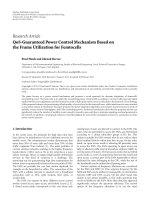
Figure 1: The SF for a single gene. The leftmost point is for k = 0,
and each subsequent vertical band corresponds to a unit increase in
k. The slope of the SF goes above
−1afterk = 2, the same indegree
for which the total codelength L
M
(y , λ, d)+L

N
(y , λ, d) is minimized.
ability to identify predecessor sets of arbitrary size. The
SF was originally developed within the algorithmic theory
of complexity and is noncomputable, so, in order to use
this theory for statistical modeling, we need a computable
alternative. The details are beyond the scope of this paper,
but obtaining a computable SF requires, for fixed λ,par-
titioning the parameter space for Θ so that the Kullback-
Leibler distance between any two adjacent partitions, each
of which represents a different model, is d/n for some d
[21]. When using an NML model class, this partitioning
yields an asymptotically uniform prior so that any model
P(y; λ, f ,X, Θ) can be encoded with length
L
M
(y, λ, d) =

l:b
l
∈X
log C
m
l
+
w
2
log
wπ
2d

+ L
λ
, (17)
where w
≤ 2
k
is the number of error estimates in

Θ [21].
Again, the inequality is necessary for data in which not all
possible regressor vectors are observed. The partitioning also
increases the noise codelength [21]to
L
N
(y, λ, d) =−log P

y; λ,

f , X,

Θ

+
d
2
. (18)
We ref er to L
M
and L
N

as the model and noise codelengths,
respectively, which together constitute a universal sufficient
statistics decomposition of the total codelength. The sum-
mation of these values is clearly different from the stochastic
complexity, but this is a result of partitioning the parameter
space.
The appropriate analogue of the SF is then defined as
h
y
(α) = min
λ,d

L
N
(y, λ, d):L
M
(y, λ, d) ≤ α

. (19)
We see that h
y
(α) is a nonincreasing function of the model
constraint α and displays the minimum possible amount of
noise in the data if we restrict the model codelength to be less
than α. Rissanen shows that this criterion is minimized for
d
= w [21], but the optimal λ cannot be solved analytically.
However, by plotting h
y
(α) we obtain a graph similar to a

rate-distortion curve (Figure 1), and by making a convex hull
we can find a near-optimal predecessor set. Simply select the
truncation point at which the magnitude of the slope of the
hull drops below 1. In other words, locate the truncation
point at which allowing an additional bit for the model yields
less than a 1-bit reduction in the noise codelength because,
once past this point, increasing the model complexity no
longer decreases the total encoding cost.
Of particular use in this scenario is the way in which the
model codelength is somewhat stable for each k, producing
the distinct bands in Figure 1. The noise codelengths are still
widely dispersed so we are required to compute all possible
codelengths up to some total number of predecessors. We
would like that number to be variable and not arbitrarily
specified in advance, but this may not be feasible for highly
connected networks. However, as mentioned earlier, the
indegrees of genetic networks are generally assumed to be
small (hence, the standard K
= 3), and, when looking for a
single gene’s predecessors in a 20-gene network, our method
only takes 70 minutes to check every possible set up to size
6. Thus, we are still constrained by a maximum indegree, but
we can now increase it well beyond the accepted number that
we expect to encounter in practice without risking extreme
computational repercussions. Additionally, choosing a K
≤
g/2makesL
λ
a nondecreasing function of k, meaning that
we can also stop searching if L

λ
ever becomes larger than
the current value of L
M
(y,

λ, d)+L
N
(y,

λ, d). The method is
summarized in Algorithm 1.
Note that we termed the resulting predecessors “near-
optimal.” It is possible to encounter genes for which adding
one predecessor does not warrant an increase in model
codelength but adding two predecessors does. Nevertheless,
these differences tend to be small for certain types of
networks. Moreover, depending on the kind of error with
which one is concerned, these near-optimal predecessor sets
can even provide a better approximation of the true network
in the sense that any differences will be in the direction of the
SF finding fewer predecessors. Thus, assuming a maximum
indegree K, the false positive rate from using the SF can never
be higher than that from checking all predecessor sets up to
size K.
3. Results
3.1. Performance on Simulated Data
A critical issue in performance analysis concerns the class
from which the random networks are to be generated. While
it might first appear that one should generate networks using

the class G
g
composed of all Boolean networks containing
g genes, this is not necessarily the case if one wishes to
achieve simulated results that reflect algorithm performance
6 EURASIP Journal on Bioinformatics and Systems Biology
(1) Initialize

λ ⇐ ∅
(2) L
N
(

λ) ⇐ nh(sum(y)/n)+1/2
(3) L
M
(

λ) ⇐ log C
n
+(1/2) log(π/2) + log(1 + lng)
(4) for k
= 1toK do
(5) compute L
λ
using (16)
(6) if L
λ
>L
M

(

λ)+L
N
(

λ) then
(7) return

λ
(8) end if
(9) H
⇐ collection of all λ’s such that |λ|=k
(10) for i
= 1to|H|do
(11) X
i
⇐ rows of X specified by H
i
(12) for l = 1to2
k
do
(13) compute m
l
and m
l
1
for X
i
(14) end for

(15) w, d
⇐ number of nonzero m
l
’s
(16) compute L
N
(H
i
)andL
M
(H
i
)
using (11), (17), and (18)
(17) end for
(18) use L
N
, L
M
, L
N
(

λ), and L
M
(

λ)toformaconvex
hull with truncation points
{(tpM

j
, tpN
j
)}
(19) idx ⇐ max
j
{(j : tpN
j
−tpN
j−1
)/
(tpM
j
−tpM
j−1
) < −1}
(20) if isempty (idx) then
(21) return

λ
(22) else
(23) update

λ, L
N
(

λ), and L
M
(


λ) using truncation
point indexed by idx
(24) end if
(25) end for
Algorithm 1: The NML MDL method for one gene.
on realistic networks. An obvious constraint is to limit the
indegree, either for biological reasons [26] or for the sake of
inference accuracy when data are limited. In this case, one
can consider the class G
κ
g
composed of all Boolean networks
with indegrees bounded by κ. Other constraints might
include realistic attractor structures [27], networks that are
neither too sensitive nor too insensitive to perturbations
[28], or networks that are neither too chaotic nor too ordered
[29].
Here we consider a constraint on the functions that is
known to prevent chaotic behavior [5, 26]. A canalizing
function is one for which there exists a gene among its
regulatory set such that if the gene takes on a certain
value, then that value determines the value of the function
irrespective of the values of the other regulatory genes. For
example, f (x
1
, x
2
, x
3

) = (x
1
and x
3
)ORx
3
is canalizing
with respect to x
3
because f (x
1
, x
2
,1) = 1 for any values
of x
1
and x
2
. There is evidence that genetic networks under
the Boolean model favor this kind of functionality [30].
Corresponding to class G
κ
g
is class C
κ
g
, in which all functions
are constrained to be canalizing.
To evaluate the performance of our model selection
method, referred to as NML MDL, on synthetic Boolean

networks, we consider sample sizes ranging from 20 to 100,
θ
∈{0.1, 0.2, 0.3},andκ ∈{1, 2,3, 4}. We test each of the
(n, θ, κ) combinations on 30 randomly generated networks
from G
κ
20
and C
κ
20
. Note that G
1
20
is equivalent to C
1
20
.
We use the Reveal and Network MDL methods as
benchmarks for comparison. As mentioned earlier, Net-
work MDL requires a tuning parameter, which we set to
0.3 since that paper uses 0.2–0.4 as the range for this
parameter in its simulations. Also, its application in [10]
limits the average indegree of the inferred network to 3
so we assume this as well. Reveal is run from a Matlab
toolbox created by Kevin Murphy, available for download at
and requires a fixed K,whichwe
also set to 3. We implement our method with and without
including the SF approach to show that the difference in
accuracy is often small, especially in light of the reduction
in computation time.

As performance metrics, we use the number of false
positives and the Hamming distance between the estimated
and true networks, both normalized over the total number
of edges in the true network. False positives are defined as
any time a proposed network includes an edge not existing
in the real network, and Hamming distance is defined as the
number of false positives plus the number of edges in the true
network not included in the estimated network.
3.1.1. Random Networks
In this section, we consider performance when the net-
work is generated from G
κ
20
. Figures 2–5 show a selection
of the performance-metric results for all four methods
and several combinations of κ and θ. The remaining
figures can be found in the supporting data, available at
/>∼jdougherty/nmlmdl.
With respect to false positives, NML MDL is uniformly
the best, and there is at most a minor difference between
the two modes. NML MDL is also the best overall method
when looking at Hamming distances. Figures 2 and 3 show
the cases for which it most definitively improves upon
Network MDL and Reveal, both of which have θ
= 0.1.
The way in which the two NML methods diverge as κ
increases is a general trend, but both remain below Network
MDL. Increasing θ to 0.2 narrows the margins between the
methods, but the relationships only change significantly for
κ

= 4. As shown in Figure 4, NML MDL with the SF loses its
edge, but NML MDL with fixed K remains the best choice.
Raising θ to 0.3 is most detrimental to Reveal, pulling its
accuracy well away from the other three methods. Figure 5
shows this for κ
= 4, but the plots for smaller values of
κ look very similar, especially in how the two NML MDL
approaches perform almost identically. We point out that this
is the worst scenario for NML MDL, but, even then, it is still
superior for small n and only worse than Network MDL for
n
= 80.
In terms of computation time, Reveal was fairly constant
for all of the simulation settings, taking an average of 6.35
seconds to find predecessors for gene using Matlab on a
Pentium IV desktop computer with 1GB of memory. NML
MDL with K
= 3 increases slightly with n in a linear fashion,
but its most noticeable increase is with κ.Forκ
= 1, this
method took an average of 0.33 to 0.48 seconds per gene as
EURASIP Journal on Bioinformatics and Systems Biology 7
0.4
0.5
0.6
0.7
0.8
0.9
1
1.1

Normalized Hamming distance
20 30 40 50 60 70 80 90 100
Sample size
NML MDL w/K
= 3
NML MDL w/SF
Network MDL
Reveal
(a)
0
0.1
0.2
0.3
0.4
0.5
Normalized false positive count
20 30 40 50 60 70 80 90 100
Sample size
NML MDL w/K
= 3
NML MDL w/SF
Network MDL
Reveal
(b)
Figure 2: (a) Hamming distances and (b) false positive counts for random networks generated from G
3
20
with θ = 0.1. Results are normalized
over the true number of connections and averaged over 30 networks.
0.4

0.5
0.6
0.7
0.8
0.9
1
1.1
Normalized Hamming distance
20 30 40 50 60 70 80 90 100
Sample size
NML MDL w/K
= 3
NML MDL w/SF
Network MDL
Reveal
(a)
0
0.05
0.1
0.15
0.2
0.25
0.3
0.35
Normalized false positive count
20 30 40 50 60 70 80 90 100
Sample size
NML MDL w/K
= 3
NML MDL w/SF

Network MDL
Reveal
(b)
Figure 3: Error rates for G
4
20
and θ = 0.1.
n goes from 20 to 100, but this range increased from 0.59
to 0.73 for κ
= 4. Alternatively, Network MDL’s runtime is
sporadic with respect to n and decreases when κ is raised,
taking an average of 2.50 seconds per gene for κ
= 1but
needing only 0.33 second per gene when κ
= 4, the only case
for which it was noticeably faster than NML MDL with fixed
K. However, NML MDL with the SF proved to be the most
efficient algorithm in almost every scenario. For θ
= 0.2and
0.3 it was uniformly the fastest, taking an average of 0.06 and
0.02 seconds per gene, respectively. The runtime begins to
increase more rapidly with n for θ
= 0.1andκ ≥ 3, but the
only observed case when it was not the fastest method was
for n
= 100 and κ = 4, and even then the needed time was
still less than 1 second per gene.
3.1.2. Canalizing Networks
Next, we impose the canalizing restriction and generate
networks from C

κ
20
. The general impact can be seen by
comparing Figures 3 and 6. There is essentially no difference
8 EURASIP Journal on Bioinformatics and Systems Biology
0.6
0.7
0.8
0.9
1
1.1
1.2
1.3
Normalized Hamming distance
20 30 40 50 60 70 80 90 100
Sample size
NML MDL w/K
= 3
NML MDL w/SF
Network MDL
Reveal
(a)
0
0.1
0.2
0.3
0.4
0.5
Normalized false positive count
20 30 40 50 60 70 80 90 100

Sample size
NML MDL w/K
= 3
NML MDL w/SF
Network MDL
Reveal
(b)
Figure 4: Error rates for G
4
20
and θ = 0.2.
0.8
0.9
1
1.1
1.2
1.3
1.4
1.5
1.6
Normalized Hamming distance
20 30 40 50 60 70 80 90 100
Sample size
NML MDL w/K
= 3
NML MDL w/SF
Network MDL
Reveal
(a)
0

0.1
0.2
0.3
0.4
0.5
0.6
0.7
Normalized false positive count
20 30 40 50 60 70 80 90 100
Sample size
NML MDL w/K
= 3
NML MDL w/SF
Network MDL
Reveal
(b)
Figure 5: Error rates for G
4
20
and θ = 0.3.
in the false positive rates (or runtimes), but the behavior of
the Hamming distances is clearly different. We observe that
NML MDL with fixed K performs better over all Boolean
functions, although invoking the SF yields error rates much
closer to the fixed K approach when we are restricted to
canalizing functions. This is expected because one canalizing
gene can provide a significant amount of predictive power,
whereas a noncanalizing function may require multiple
predecessors to achieve any amount of predictability.
For example, consider f (x

1
, x
2
) = x
1
OR x
2
.Ifx
1
is found
to be the best predecessor set of size 1, adding x
2
may not
give enough additional information to warrant the increased
model codelength, in which case NML MDL will miss one
connection. Alternatively, if f (x
1
, x
2
) = x
1
XOR x
2
, either
input tells almost nothing by itself, and the SF will probably
stop the inference too soon. However, using both inputs will
most likely result in the minimum total codelength, in which
case NML MDL with fixed K will find the correct predecessor
set.
For the same reason, we also see that Network MDL

is better suited to canalizing functions, but Reveal does
better without this constraint. Of particular interest is that,
EURASIP Journal on Bioinformatics and Systems Biology 9
0.5
0.6
0.7
0.8
0.9
1
1.1
Normalized Hamming distance
20 30 40 50 60 70 80 90 100
Sample size
NML MDL w/K
= 3
NML MDL w/SF
Network MDL
Reveal
(a)
0
0.05
0.1
0.15
0.2
0.25
0.3
0.35
Normalized false positive count
20 30 40 50 60 70 80 90 100
Sample size

NML MDL w/K
= 3
NML MDL w/SF
Network MDL
Reveal
(b)
Figure 6: Error rates for C
4
20
and θ = 0.1.
runt
Antp
grh
hkb
opa
abd-A
Te a s h i r t
Bicoid
Tinman
Tw ist
Eve
Paired
Odd
Wingless
Stat92E
Notch
Ta il le ss
tkv
dpp
Brinker

Previously verified
Follows hierarchy
Active in same area
Unconfirmed
Figure 7: Inferred gene regulatory network for Drosophila.
for these methods, the change can be so drastic that they
comparatively switch their rankings depending on which
network class we use, whereas NML MDL provides the most
accurate inference either way. Similar results can be observed
for the other cases in the supporting data. Based on these
findings, we recommend using the SF primarily for networks
composed of canalizing functions and networks too large
to run NML MDL with fixed K in a reasonable amount of
time. We also suggest using the SF when θ is large because,
as pointed out in Section 3.1.1, the performance of the two
NMLMDLvarietiesisnolongerdifferent when θ
= 0.3.
3.2. Application to Drosophila Data
In order to examine the proficiency of NML MDL on real
data, we tested it on time-series Drosophila gene expression
measurements made by Arbeitman et al. [31]. The dataset
10 EURASIP Journal on Bioinformatics and Systems Biology
in question consists of 4028 genes observed over 67 time
points, which we binarized according to the procedure
outlined in [10]. We selected 20 of these genes based on
type (gap, pair-rule, etc.) and the availability of genetically
verified directed interactions in the literature. Of the 32 edges
identified by NML MDL (Figure 7), 16 have been previously
demonstrated [32–43], and 3 more follow the standard
genetic hierarchy [44]. Observe that 3 of the 12 other edges

are simply reversals of known relationships and, therefore,
could possibly represent unknown feedback mechanisms.
Additionally, 5 of the remaining inferred relationships are
between genes that are active in the same area such as the
central nervous system (Antp/runt) and reproductive organs
(Notch/paired) (the Interactive Fly website, hosted by the
Society for Developmental Biology).
4. Concluding Remarks
Using a universal codelength when applying the MDL
principle eliminates the relativity of applying ad hoc code-
lengths and user-defined tuning parameters. In our case,
this has resulted in improved accuracy of Boolean network
esimation. Using the theoretically grounded stochastic com-
plexity instead of ad hoc encodings genuinely reflects the
intent of the MDL principle. In addition, the structure
function makes the proposed method faster than other
published methods. Computation time does not heavily rely
on bounded indegrees and increases only slightly with n.
Acknowledgments
This work was supported by the Academy of Finland
(Application no. 213462, Finnish Programme for Centres
of Excellence in Research 2006–2011), and the Tampere
Graduate School in Information Science and Engineering.
Partial support also provided by the National Cancer Insti-
tute (Grant no. CA90301).
References
[1] J. Pearl, Probabilistic Reasoning in Intelligent Systems: Networks
of Plausible Inference, Morgan Kaufmann, San Francisco, Calif,
USA, 1988.
[2] N. Friedman, M. Linial, I. Nachman, and D. Pe’er, “Using

Bayesian networks to analyze expression data,” Journal of
Computational Biology, vol. 7, no. 3-4, pp. 601–620, 2000.
[3] T. Dean and K. Kanazawa, “A model for reasoning about
persistence and causation,” Computational Intelligence, vol. 5,
no. 2, pp. 142–150, 1989.
[4] K. Murphy, “Dynamic Bayesian networks: representation,
inference and learning,” Ph.D. thesis, Computer Science
Division, UC Berkeley, Berkeley, Calif, USA, 2002.
[5] S. A. Kauffman, “Metabolic stability and epigenesis in ran-
domly constructed genetic nets,” Journal of Theoretical Biology,
vol. 22, no. 3, pp. 437–467, 1969.
[6] I. Shmulevich, E. R. Dougherty, S. Kim, and W. Zhang,
“Probabilistic Boolean networks: a rule-based uncertainty
model for gene regulatory networks,” Bioinformatics, vol. 18,
no. 2, pp. 261–274, 2002.
[7] H. L
¨
ahdesm
¨
aki, S. Hautaniemi, I. Shmulevich, and O. Yli-
Harja, “Relationships between probabilistic Boolean networks
and dynamic Bayesian networks as models of gene regulatory
networks,” Signal Processing, vol. 86, no. 4, pp. 814–834, 2006.
[8] D. Pe’er, A. Regev, G. Elidan, and N. Friedman, “Inferring sub-
networks from perturbed expression profiles,” Bioinformatics,
vol. 17, supplement 1, pp. S215–S224, 2001.
[9] X. Zhou, X. Wang, R. Pal, I. Ivanov, M. Bittner, and E.
R. Dougherty, “A Bayesian connectivity-based approach to
constructing probabilistic gene regulatory networks,” Bioinfor-
matics, vol. 20, no. 17, pp. 2918–2927, 2004.

[10] W. Zhao, E. Serpedin, and E. R. Dougherty, “Inferring gene
regulatory networks from time series data using the minimum
description length principle,” Bioinformatics, vol. 22, no. 17,
pp. 2129–2135, 2006.
[11] S. Liang, S. Fuhrman, and R. Somogyi, “Reveal, a general
reverse engineering algorithm for inference of genetic network
architectures,” Pacific Symposium on Biocomputing, vol. 3, pp.
18–29, 1998.
[12] T. Akutsu, S. Miyano, and S. Kuhara, “Identification of genetic
networks from a small number of gene expression patterns
under the Boolean network model,” Pacific Symposium on
Biocomputing, vol. 3, pp. 17–28, 1999.
[13] I. Shmulevich, A. Saarinen, O. Yli-Harja, and J. Astola, “Infer-
ence of genetic regulatory networks via best-fit extensions,”
in Computational and Statistical Approaches to Genomics,pp.
197–210, chapter 11, Kluwer Academic Publishers, New York,
NY, USA, 2002.
[14] H. L
¨
ahdesm
¨
aki, I. Shmulevich, and O. Yli-Harja, “On learning
gene regulatory networks under the Boolean network model,”
Machine Learning, vol. 52, no. 1-2, pp. 147–167, 2003.
[15] A. A. Margolin, I. Nemenman, K. Basso, et al., “ARACNE: An
algorithm for the reconstruction of gene regulatory networks
in a mammalian cellular context,” BMC Bioinformatics, vol. 7,
supplement 1, p. S7, 2006.
[16] I. Nemenman, “Information theory, multivariate dependence,
and genetic network inference,” Tech. Rep. NSF-KITP-04-54,

KITP, UCSB, Santa Barbara, Calif, USA, June 2004.
[17] J. Rissanen, “Modeling by shortest data description,” Automat-
ica, vol. 14, no. 5, pp. 465–471, 1978.
[18] J. Rissanen, “Stochastic complexity and modeling,” Annals of
Statistics, vol. 14, no. 3, pp. 1080–1100, 1986.
[19] V. Vapnik, Estimation of Dependencies Based on Empirical
Data, Springer, New York, NY, USA, 1982.
[20] I. Tabus and J. Astola, “On the use of MDL principle in gene
expression prediction,” EURASIP Journal on Applied Signal
Processing, vol. 2001, no. 4, pp. 297–303, 2001.
[21] J. Rissanen, Information and Complexity in Statistical Model-
ing, Springer, New York, NY, USA, 2007.
[22] A. Wuensche, “Genomic regulation modeled as a network
with basins of attraction,” Pacific Symposium on Biocomputing,
vol. 3, pp. 89–102, 1998.
[23] I. Tabus, J. Rissanen, and J. Astola, “Normalized maximum
likelihood models for Boolean regression with application to
prediction and classification in genomics,” in Computational
and Statistical Approaches to Genomics, pp. 173–196, chapter
10, Kluwer Academic Publishers, New York, NY, USA, 2002.
[24] W. Szpankowski, “On asymptotics of certain recurrences aris-
ing in universal coding,” Problems of Information Transmission,
vol. 34, no. 2, pp. 55–61, 1998.
[25] D. Thieffry,A.M.Huerta,E.P
´
erez-Rueda, and J. Collado-
Vides, “From specific gene regulation to genomic networks:
a global analysis of transcriptional regulation in Escherichia
coli,” BioEssays, vol. 20, no. 5, pp. 433–440, 1998.
EURASIP Journal on Bioinformatics and Systems Biology 11

[26] S. A. Kauffman, The Origins of Order, Oxford University Press,
Oxford, UK, 1993.
[27] R.Pal,I.Ivanov,A.Datta,M.L.Bittner,andE.R.Dougherty,
“Generating Boolean networks with a prescribed attractor
structure,” Bioinformatics, vol. 21, no. 21, pp. 4021–4025,
2005.
[28] I. Shmulevich and S. A. Kauffman, “Activities and sensitivities
in Boolean network models,” Physical Review Letters, vol. 93,
no. 4, Article ID 86394, 4 pages, 2004.
[29] B. Derrida and Y. Pomeau, “Random networks of automata:
a simple annealed approximation,” Europhysics Letters, vol. 1,
pp. 45–49, 1986.
[30] S. Harris, B. Sawhill, A. Wuensche, and S. A. Kauffman, “A
model of transcriptional regulatory networks based on biases
in the observed regulation rules,” Complexit y,vol.7,no.4,pp.
23–40, 2002.
[31] M. Arbeitman, E. Furlong, F. Imam, et al., “Gene expression
during the life cycle of Drosophila melanogaster,” Science,
vol. 297, no. 5590, pp. 2270–2275, 2002.
[32] J. Bhojwani, L. S. Shashidhara, and P. Sinha, “Requirement
of teashirt (tsh) function during cell fate specification in
developing head structures in Drosophila,” De velopment Genes
and Evolution, vol. 207, no. 3, pp. 137–146, 1997.
[33] D. M. Cimbora and S. Sakonju, “Drosophila midgut morpho-
genesis requires the function of the segmentation gene odd-
paired,” Developmental Biology, vol. 169, no. 2, pp. 580–595,
1995.
[34] M. Fujioka, J. Jaynes, and T. Goto, “Early even-skipped stripes
act as morphogenetic gradients at the single cell level to
establish engrailed expression,” Development, vol. 121, no. 12,

pp. 4371–4382, 1995.
[35] M. Gonz
´
alez-Gaitan and H. J
¨
ackle, “Invagination centers
within the Drosophila stomatogastric nervous system anlage
are positioned by Notch-mediated signaling which is spatially
controlled through wingless,” Development, vol. 121, no. 8, pp.
2313–2325, 1995.
[36] L. D. Mathies, S. Kerridge, and M. P. Scott, “Role of the teashirt
gene in Drosophila midgut morphogenesis: secreted proteins
mediate the action of homeotic genes,” Development, vol. 120,
no. 10, pp. 2799–2809, 1994.
[37]S.Morimura,L.Maves,Y.Chen,andF.M.Hoffmann,
“Decapentaplegic overexpression affects Drosophila
wing and
leg imaginal disc development and wingless expression,”
De velopmental Biology, vol. 177, no. 1, pp. 136–151, 1996.
[38] B. S L. Dr
´
ean, A. Nasiadka, J. Dong, and H. M. Krause,
“Dynamic changes in the functions of Odd-skipped dur-
ing early Drosophila embryogenesis,” Development, vol. 125,
no. 23, pp. 4851–4861, 1998.
[39] V. Schaeffer, D. Killian, C. Desplan, and E. A. Wimmer,
“High Bicoid levels render the terminal system dispensable for
Drosophila head development,” De velopment, vol. 127, no. 18,
pp. 3993–3999, 2000.
[40] P. Steneberg, J. Hemph

¨
al
¨
a, and C. Samakovlis, “Dpp and
Notch specify the fusion cell fate in the dorsal branches of
the Drosophila trachea,” Mechanisms of Development, vol. 87,
no. 1-2, pp. 153–163, 1999.
[41] I. S. Torres, H. L
´
opez-Schier, and D. St. Johnston, “A
Notch/Delta-dependent relay mechanism establishes anterior-
posterior polarity in Drosophila,” Developmental Cell, vol. 5,
no. 4, pp. 547–558, 2003.
[42] J. Torres-Vazquez, S. Park, R. Warrior, and K. Arora, “The
transcription factor Schnurri plays a dual role in mediating
Dpp signaling during embryogenesis,” Development, vol. 128,
no. 9, pp. 1657–1670, 2001.
[43] Z. Yin, X L. Xu, and M. Frasch, “Regulation of the twist target
gene tinman by modular cis-regulatory elements during early
mesoderm development,” Development, vol. 124, no. 24, pp.
4971–4982, 1997.
[44] M. D. Schroeder, M. Pearce, J. Fak, et al., “Transcriptional
control in the segmentation gene network of Drosophila,” PLoS
Biology, vol. 2, no. 9, p. e271, 2004.