Báo cáo hóa học: "Research Article Adaptive Kernel Canonical Correlation Analysis Algorithms for Nonparametric Identification of Wiener and Hammerstein Systems" potx

Hindawi Publishing Corporation
EURASIP Journal on Advances in Signal Processing
Volume 2008, Article ID 875351, 13 pages
doi:10.1155/2008/875351
Research Article
Adaptive Kernel Canonical Correlation Analysis
Algorithms for Nonparametric Identification of Wiener
and Hammerstein Systems
Steven Van Vaerenbergh, Javier V
´
ıa, and Ignacio Santamar
´
ıa
Department of Communications Engineering, University of Cantabria, 39005 Santander, Cantabria, Spain
Correspondence should be addressed to Steven Van Vaerenbergh,
Received 1 October 2007; Revised 4 January 2008; Accepted 12 February 2008
Recommended by Sergios Theodoridis
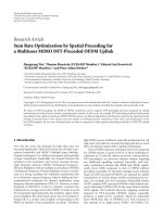
This paper treats the identification of nonlinear systems that consist of a cascade of a linear channel and a nonlinearity, such as the
well-known Wiener and Hammerstein systems. In particular, we follow a supervised identification approach that simultaneously
identifies both parts of the nonlinear system. Given the correct restrictions on the identification problem, we show how kernel
canonical correlation analysis (KCCA) emerges as the logical solution to this problem. We then extend the proposed identification
algorithm to an adaptive version allowing to deal with time-varying systems. In order to avoid overfitting problems, we discuss
and compare three possible regularization techniques for both the batch and the adaptive versions of the proposed algorithm.
Simulations are included to demonstrate the effectiveness of the presented algorithm.
Copyright © 2008 Steven Van Vaerenbergh et al. This is an open access article distributed under the Creative Commons
Attribution License, which permits unrestricted use, distribution, and reproduction in any medium, provided the original work is
properly cited.
1. INTRODUCTION
In recent years, a growing amount of research has been done
on nonlinear system identification [1, 2]. Nonlinear dynami-
cal system models generally have a high number of param-

eters although many problems can be sufficiently well ap-
proximated by simplified block-based models consisting of
a linear dynamic subsystem and a static nonlinearity. The
model consisting of a cascade of a linear dynamic system and
a memoryless nonlinearity is known as the Wiener system,
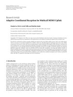
while the reversed model (a static nonlinearity followed by a
linear filter) is called the Hammerstein system. These systems
are illustrated in Figures 1 and 2, respectively. Wiener sys-
tems are frequently used in contexts such as digital satellite
communications [3], digital magnetic recording [4], chemi-
cal processes, and biomedical engineering. Hammerstein sys-
tems are, for instance, encountered in electrical drives [5]
and heat exchangers.
Thepastdecadehasseenanumberofdifferent ap-
proaches to identify these systems, which can generally be
divided into three classes. First attempts followed a black-
box approach where traditionally the problem of nonlin-
ear equalization or identification was tackled by considering
nonlinear structures such as multilayer perceptrons (MLPs)
[6], recurrent neural networks [3], or piecewise linear net-
works [7]. A second approach is the two-step method, which
exploits the system structure to consecutively or alternatingly
estimate the linear part and the static nonlinearity. Most pro-
posed two-step techniques are based on predefined test sig-
nals [8, 9]. A third method is the simultaneous estimation
of both blocks, adopted, for instance, in [10, 11], and the it-
erative method in [12]. Although all above-mentioned tech-
niques are supervised approaches (i.e., input and output sig-
nals are known during estimation), recently, there have also
been a few attempts to unsupervised identification [13, 14].

In this paper, we focus on the problem of supervised
Wiener and Hammerstein system identification, simultane-
ously estimating the linear and nonlinear parts. Following an
idea introduced in [10], we estimate one linear filter and one
memoryless nonlinearity representing the two system blocks
and obtain an estimate of the signal in between these blocks.
To minimize the estimation error, we use a different criterion
than the one in [10]: instead of constraining the norm of the
estimated filters, we fix the norm of the output signals for
each block, which, as we show, leads to an algorithm that is
more robust to noise.
2 EURASIP Journal on Advances in Signal Processing
x[n] H(z)
r[n]
f (·)
s[n]
v[n]
+
y[n]
Figure 1: A Wiener system with additive noise v[n].
The main contributions of this paper are twofold. First,
we demonstrate how the chosen constraint leads to an im-
plementation of the well-known kernel canonical correlation
analysis (KCCA or kernel CCA) algorithm. Second, we show
how the KCCA solution allows to formulate this problem as
a set of two coupled least-squares (LS) regression problems
that can be solved in an iterative manner, which is exploited
to develop an adaptive KCCA algorithm. The resulting al-
gorithm is capable of identifying systems that change over
time. To avoid the overfitting problems that are inherent to

the use of kernel methods, we discuss and compare three reg-
ularization techniques for the batch and adaptive versions of
the proposed algorithm.
Throughout this paper, the following notation will be
adopted: scalars will be denoted in lowercase as x,vectorsin
bold as x and matrices will be bold uppercase letters such as
X. Vectors will be used in column format unless otherwise
mentioned, and data matrices X are constructed by stacking
data vectors as rows of this matrix. Data points that are trans-
formed into feature space will be represented with a tilde, for
instance,
x. If all (row-wise stored) points of a data matrix
X are transformed into feature space, the resulting matrix is
denoted as

X.
The remainder of this paper is organized as follows.
Section 2 describes the identification problem and the pro-
posed identification criterion. A detailed description of the
algorithm and the options to regularize its solutions are given
in Section 3, which concludes with indications of how this
algorithm can be used to perform full Wiener and Ham-
merstein system identification and equalization. The exten-
sion to the adaptive algorithm is made in Section 4, and in
Section 5, the performance of the algorithm is illustrated by
simulation examples. Finally, Section 6 summarizes the main
conclusions of this work.
2. PROBLEM STATEMENT AND PROPOSED
IDENTIFICATION CRITERION
Wiener and Hammerstein systems are two similar low-

complexity nonlinear models. The Wiener system consists of
a series connection of a linear channel and a static nonlinear-
ity (see Figure 1). The Hammerstein system, its counterpart,
is a cascade of a static nonlinearity and a linear channel (see
Figure 2).
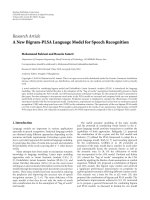
Recently, an iterative gradient identification method was
presented for Wiener systems [10] that exploits the cascade
structure by jointly identifying the linear filter and the inverse
nonlinearity. It uses a linear estimator

H(z) and a nonlinear
estimator g(
·), that, respectively, model the linear filter H(z)
and the inverse nonlinearity f
−1
(·), as depicted in Figure 3,
x[n]
f (
·)
r[n]
H(z)
s[n]
v[n]
+
y[n]
Figure 2: A Hammerstein system with additive noise.
x[n]

H(z)
r

x
[n]
−
r
y
[n]
e[n]
g(
·)
y[n]
Figure 3: The used Wiener system identification diagram.
assuming that the nonlinearity f (·) is invertible in the out-
put data range. The estimator models are adjusted by mini-
mizing the error e[n] between their outputs r
x
[n]andr
y
[n].
In the noiseless case, it is possible to find estimators whose
outputs correspond exactly to the reference signal r[n](up
to an unknown scaling factor which is inherent to this prob-
lem).
In order to avoid the zero-solution

H(z) = 0and
g(
·) = 0, which obviously minimizes e[n], a certain con-
straint should be applied to the solutions. For that purpose,
it is instructive to look at the expanded form
e

2
=


r
x
− r
y


2
=


r
x


2
+


r
y


2
− 2r
T
x

r
y
,(1)
where e, r
x,
and r
y
are vectors that contain all elements
e[n], r
x
[n], and r
y
[n], respectively, with n = 1, , N.
In [10], a linear restriction was proposed to avoid zero
solutions of (1): the first coefficient of the linear filter

H(z)
was fixed to 1, thus fixing the scaling factor and also the norm
of all filter coefficients. With the estimated filter represented
as h
= [h
1
, , h
L
], the minimization problem reads
min


r
x

− r
y


2
s.t.h
1
= 1. (2)
However, from (1), it is easy to see that any such restriction
on the filter coefficients will not necessarily prevent the terms
r
x

2
and r
y

2
from going to zero, hence possibly leading
to noise enhancement problems. For instance, if a low-pass
signal is fed into the system, the cost function (2)willnot
exclude the possibility that the estimated filter

H(z)exactly
cancels this signal, as would do a high-pass filter.
A second and more sensible restriction to minimize (1)is
to fix the energy of the output signals r
x
and r
y

while maxi-
mizing their correlation r
T
x
r
y
, which is obtained by solving
min


r
x
− r
y


2
s.t.


r
x


2
=


r
y



2
= 1. (3)
Since the norms of r
x
and r
y
are now fixed, the zero solution
is excluded per definition. To illustrate this, a direct perfor-
mance comparison between batch identification algorithms
based on filter coefficient constraints and this signal power
constraint will be given in Section 5.1.
Steven Van Vaerenbergh et al. 3
3. KERNEL CANONICAL CORRELATION ANALYSIS
FOR WIENER SYSTEM IDENTIFICATION
In this section, we will construct an identification algorithm
based on the proposed signal power constraint (3). To rep-
resent the linear and nonlinear estimated filters, different ap-
proaches can be used. We will use an FIR model for the linear
part of the system. For the nonlinear part, a number of para-
metric models can be used, including power series, Cheby-
shev polynomials, wavelets and piecewise linear (PWL) func-
tions, as well as some nonparametric methods including neu-
ral networks. Nonparametric approaches do not assume that
the nonlinearity corresponds to a given model, but rather let
the training data decide which characteristic fits them best.
We will apply a nonparametric identification approach based
on kernel methods.
3.1. Kernel methods

Kernel methods [15] are powerful machine learning tech-
niques built on the framework of reproducing kernel Hilbert
spaces (RKHS). They are based on a nonlinear transforma-
tion Φ of the data from the input space to a high-dimensional
feature space H , where it is more likely that the problem can
be solved in a linear manner [16],
Φ :
R
m
−→ H, Φ(x) = x. (4)
However, due to its high dimensionality, it is hard or even
impossible to perform calculations directly in this feature
space. Fortunately, scalar products in feature space can be
calculated without the explicit knowledge of the nonlinear
transformation Φ. This is done by applying the correspond-
ing kernel function κ(
·, ·) on pairs of data points in the input
space,
κ

x
i
, x
j

:=

x
i
, x

j

=

Φ

x
i

, Φ

x
j

. (5)
This property, which is known as the “kernel trick,” allows
to perform any scalar product-based algorithm in the fea-
ture space by solely replacing the scalar products with the
kernel function in the input space. Commonly used kernel
functions include the Gaussian kernel with width σ,
κ

x
i
, x
j

=
exp


−


x
i
− x
j


2
2σ
2

,(6)
which implies an infinite dimensional feature space [15], and
the polynomial kernel of order p,
κ

x
i
, x
j

=

x
T
i
x
j

+ c

p
,(7)
where c is a constant.
3.2. Identification algorithm
To identify the linear channel of the Wiener system, we will
estimate an FIR filter h
∈ R
L
whose output is given by
r
x
[n] = x[n]
T
h,(8)
where x[n]
= [x[n], x[n − 1], , x[n − L +1]]
T
∈ R
L
is a
time-embedded vector. For the nonlinear part, we will look
for a linear solution in the feature space, which corresponds
to a nonlinear solution in the original space. This solution is
represented as the vector

h
y
∈ R

m

, which projects the trans-
formed data point
y[n] = Φ(y[n]) onto
r
y
[n] = g(y[n]) = y[n]
T

h
y
. (9)
According to the representer theorem [17], the optimal

h
y
can be obtained as a linear combination of the N trans-
formed data patterns, that is,

h
y
=
N

i=1
α
i
y[i]. (10)
This allows to rewrite (9)as

r
y
[n] =
N

i=1
α
i
y[n]
T
y[i] =
N

i=1
α
i
κ(y[n], y[i]), (11)
where we applied the kernel trick (5) in the second equal-
ity. Hence we obtain a nonparametric representation of the
inverse nonlinearity as the kernel expansion,
g(
·) =
N

i=1
α
i
κ(·, y[i]). (12)
Thanks to the kernel trick, we only need to estimate the N
expansion coefficients α

i
instead of the m

coefficients of

h
y
,
for which usually holds that N
 m

.
To find these optimal linear and nonlinear estimators,
it is convenient to formulate (3) in terms of matrices. By
X
∈ R
N×L
, we will denote the data matrix containing x[n]
as rows. The vector containing the corresponding outputs of
the linear filter is then obtained as
r
x
= Xh. (13)
In a similar fashion, the transformed data points
y[n]canbe
stacked to form the transformed data matrix

Y ∈ R
N×m


. The
vector containing all outputs of the nonlinear estimator is
r
y
=

Y

h
y
. (14)
Using (11), this can be rewritten as
r
y
= K
y
α, (15)
where K
y
is the kernel matrix with elements K
y
(i, j) =
κ(y[i], y[j]), and α is a vector containing all coefficients α
i
.
This also allows us to write K
y
=

Y


Y
T
and

h
y
=

Y
T
α.
With the obtained data representation, the minimization
problem (3) is rewritten as minimizing
min


Xh − K
y
α


2
s.t. Xh
2
=


K
y

α


2
= 1. (16)
4 EURASIP Journal on Advances in Signal Processing
This problem is a particular case of kernel canonical correla-
tion analysis (KCCA) [18–20] in which a linear and a nonlin-
ear kernels are used. It has been proven [19] that minimizing
(16) is equivalent to maximizing
ρ
= max
r
T
x
r
y


r
x




r
y


=

max
h,α
h
T
X
T
K
y
α

h
T
X
T
Xhα
T
K
T
y
K
y
α
. (17)
If both kernels were linear, this problem would reduce to
standard linear canonical correlation analysis (CCA), which
is an established statistical technique to find linear relation-
ships between two data sets [21].
The minimization problem (16) can be solved by the
method of Lagrange multipliers, yielding the following gen-
eralized eigenvalue (GEV) problem [19, 22]:

1
2
⎡
⎣
X
T
XX
T
K
y
K
T
y
XK
T
y
K
y
⎤
⎦
⎡
⎣
h
α
⎤
⎦
=
β
⎡
⎣

X
T
X0
0K
T
y
K
y
⎤
⎦
⎡
⎣
h
α
⎤
⎦
, (18)
where β
= (ρ+1)/2 is a parameter related to a principal com-
ponent analysis (PCA) interpretation of CCA [23]. In prac-
tice, it is sufficient to solve the slightly less complex GEV
1
2
⎡
⎣
X
T
XX
T
K

y
XK
y
⎤
⎦
⎡
⎣
h
α
⎤
⎦
=
β
⎡
⎣
X
T
X0
0K
y
⎤
⎦
⎡
⎣
h
α
⎤
⎦
. (19)
As can be easily verified, the GEV problem (19)istrans-

formed into (18) by premultiplication with a block-diagonal
matrix containing the unit matrix and K
T
y
. Hence, any pair
(h, α) that solves (19) will also be a solution of (18).
The solution of the KCCA problem is given by the eigen-
vector corresponding to the largest eigenvalue of the GEV
(19). However, if K
y
is invertible, it is easy to see from (16)
that for each h satisfying
Xh
2
= 1, there exists an α =
K
−1
y
Xh that solves this minimization problem and, therefore,
also the GEV problem (19). This happens for sufficiently
“rich” kernel functions, that is, kernels that correspond to
feature spaces whose dimension m

is much higher than the
number of available data points N. For instance, in case the
Gaussian kernel is used, the feature space will have dimen-
sion m

=∞. With N unknown coefficients α
i

, the part
of (19) that corresponds to the nonlinear estimator poten-
tially suffers from an overfitting problem. In the next section,
we will discuss three different possibilities to overcome this
problem by regularizing the solutions.
3.3. Regularization techniques
Given the different options available in literature, the solu-
tions of (19) can be regularized by three basically different
approaches. First, a small constant can be added to the diag-
onal of K
y
, corresponding to simple quadratic regularization
of the problem. Second, the complexity of the matrix K
y
can
be limited directly by substituting it with a low-dimensional
approximation. Third, a smaller subset of significant points
y[n] can be used to construct a sparse approximation of K
y
,
which also yields a less complex version of this matrix. In
the following, we will discuss these three regularization ap-
proaches in detail and show how they can be used to obtain
three different versions of the proposed KCCA algorithm.
3.3.1. L
2
regularization
A common form of regularization is quadratic regularization
[24], also known as ridge regression, which is often applied in
kernel CCA [18–20]. It consists in restricting the L

2
norm of
the solution

h
y
. The second restriction in (16) then becomes
K
y
α
2
+ c

h
y

2
= 1, where c is a small constant. Introduc-
ing the regularized kernel matrix K
reg
y
= K
y
+cI,whereI is the
identity matrix, the regularized version of (17) is obtained as
ρ
= max
h,α
h
T

X
T
K
y
α

h
T
X
T
Xh

α
T
K
T
y
K
reg
y
α

, (20)
and the corresponding GEV problem now becomes [25]
1
2
⎡
⎣
X
T

XX
T
K
y
XK
y
⎤
⎦
⎡
⎣
h
α
⎤
⎦
=
β
⎡
⎣
X
T
X0
0K
reg
y
⎤
⎦
⎡
⎣
h
α

⎤
⎦
. (21)
3.3.2. Low-dimensional approximation
The complexity of the kernel matrix can be reduced by per-
forming principal component analysis (PCA) [26], which re-
sults in a kernel PCA technique [27]. This involves obtaining
the first M eigenvectors v
i
and eigenvalues s
i
of the kernel ma-
trix K
y
,fori = 1, , M, and constructing the approximated
kernel matrix
VΣV
T
≈ K
y
, (22)
where Σ is a diagonal matrix containing the M largest eigen-
values s
i
,andV contains the corresponding eigenvectors v
i
columnwise. Introducing α = V
T
α as the projection of α
onto the M-dimensional subspace spanned by the eigenvec-

tors v
i
, the GEV problem (19)reducesto
1
2
⎡
⎣
X
T
XX
T
VΣ
V
T
X Σ
⎤
⎦
⎡
⎣
h
α
⎤
⎦
=
β
⎡
⎣
X
T
X0

0 Σ
⎤
⎦
⎡
⎣
h
α
⎤
⎦
, (23)
where we have exploited the fact that V
T
V = I.
3.3.3. Sparsification of the solution
A third approach consists in finding a subset of M data points
d[i]
= y[n
i
], i = 1, , M whose images in feature space

d[i]
represent the remaining transformed points
y[n]sufficiently
well [28]. Once a “dictionary” of points d[i]isfoundaccord-
ing to a reasonable criterion, the complete set of data points

Y can be expressed in terms of the transformed dictionary as

Y ≈ A


D,whereA ∈ R
N×M
contains the coefficients of these
approximate linear combinations, and

D ∈ R
M×m

contains
the points

d[i] row-wise. This also reduces the expansion co-
efficients vector to
α = A
T
α, which now contains M ele-
ments. Introducing the reduced kernel matrix

K
y
=

D

D
T
,
Steven Van Vaerenbergh et al. 5
the following approximation can be made:
K

y
=

Y

Y
T
≈ A

K
y
A
T
. (24)
Substituting K
y
for A

K
y
A
T
in the minimization problem
(16) leads to the the GEV
1
2
⎡
⎣
X
T

XX
T
A

K
y
A
T
XA
T
A

K
y
⎤
⎦
⎡
⎣
h
α
⎤
⎦
=
β
⎡
⎣
X
T
X0
0A

T
A

K
y
⎤
⎦
⎡
⎣
h
α
⎤
⎦
.
(25)
In [28], a sparsification procedure was introduced to ob-
tain such a dictionary of significant points, albeit in an on-
line manner in the context of kernel recursive least-squares
regression (KRLS or kernel RLS). It was also shown that this
online sparsification procedure is related to kernel PCA. In
Section 4, we will adopt this online procedure to regularize
the adaptive version of the proposed KCCA algorithm.
3.4. A Unified approach to Wiener and Hammerstein
system identification and equalization
To identify the linear channel and the inverse nonlinearity
of the Wiener system, any of the regularized GEV problems
(21), (23), or (25) can be solved. Moreover, given the sym-
metric structure of the Wiener and Hammerstein systems
(see Figures 1 and 2), it should be clear that the same ap-
proach can be applied to identify the blocks of the Hammer-

stein system. To do so, the linear and nonlinear estimators
of the proposed kernel CCA algorithm need to be switched.
The resulting Hammerstein system identification algorithm
estimates the direct static nonlinearity and the inverse linear
channel, which is retrieved as an FIR filter.
Full identification of an unknown system provides an es-
timate of the system output given a certain input signal. To
fully identify the Wiener system, the presented KCCA algo-
rithm needs to be complemented with an estimate of the di-
rect nonlinearity f (
·). This nonlinearity can be obtained by
applying any nonlinear regression algorithm on the signal in
between the two blocks (whose estimate is provided by the
KCCA-based algorithm) and the given output signal y. In
particular, to stay within the scope of this paper, we propose
to obtain

f (·) as another kernel expansion as follows:

f (·) =
N

i=1
β
i
κ

·
, r
x

[i]

. (26)
Note that in practice, this nonlinear regression should use r
x
as input signal since this will be less influenced by the addi-
tive noise v on the output than r
y
, the other estimate of the
reference signal. In Section 5, the full identification process is
illustrated with some examples.
Apart from Wiener system identification, a number of al-
gorithms can be based directly on the presented KCCA al-
gorithm. In case of the Hammerstein system, KCCA already
obtains an estimate of the direct nonlinearity and the inverse
linear channel. To fully identify the Hammerstein system, the
direct linear channel needs to be estimated, which can be
done by applying standard filter inversion techniques [29].
At this point, it is interesting to note that the inversion of
the estimated linear filter can also be used in equalization
of the Wiener system [22], where the KCCA algorithm al-
ready obtained the inverse of the nonlinear block. To come
full circle, a Hammerstein system equalization algorithm can
be constructed based on the inverse linear channel estimated
by KCCA and the inverse nonlinearity that can be obtained
by performing nonlinear regression on the appropriate sig-
nals. A detailed study of these derived algorithms will be a
topic for future research.
4. ADAPTIVE SOLUTION
In a number of situations, it is desirable to have an adaptive

algorithm that can update its solution according to newly ar-
riving data. Standard scenarios include problems where the
amount of data is too high to apply a batch algorithm. An
adaptive (or online) algorithm can calculate the solution to
the entire problem by improving its solution on a sample-by-
sample basis, thereby maintaining a low computational com-
plexity. Another scenario happens when the observed prob-
lem or system is time varying. Instead of improving its so-
lution, the online algorithm must now adjust its solution to
the changing conditions. In this second case, the algorithm
must be capable of excluding the influence of less recent data,
which can be done, for instance, by introducing a forgetting
factor.
In this section, we discuss an adaptive version of kernel
CCA which can be used for online identification of Wiener
and Hammerstein systems.
4.1. Formulation of KCCA as coupled RLS problems
The special structure of the GEV problem (19)hasrecently
been exploited to obtain efficient CCA and KCCA algorithms
[22, 30, 31]. Specifically, this GEV problem can be viewed as
two coupled least-squares regression problems
βh
=

X
T
X

−1
X

T
r,
βK
y
α = r,
(27)
where
r = (r
x
+r
y
)/2 = (Xh+K
y
α)/2. This idea has been used
in [22, 32] to develop an algorithm based on the solution of
these regression problems iteratively: at each iteration t,two
LS regression problems are solved using
r(t) =
r
x
(t)+r
y
(t)
2
=
Xh(t − 1) + K
y
α(t − 1)
2
(28)

as desired output.
Furthermore, this LS regression framework was exploited
directly to develop an adaptive CCA algorithm based on the
recursive least-squares algorithm (RLS), which was shown to
converge to the CCA solution [32]. For Wiener and Ham-
merstein system identification, the adaptive solution of (27)
can be obtained by coupling one linear RLS algorithm with
one kernel RLS algorithm. Before describing the complete
adaptive algorithm in detail, we first review the different op-
tions that exist to implement kernel RLS.
6 EURASIP Journal on Advances in Signal Processing
4.2. Kernel recursive least-squares regression
As is the case with all online kernel algorithms, the design
of a kernel RLS algorithm presents some crucial difficulties
[33] that are not present in standard online settings for lin-
ear methods. Apart from the previously mentioned prob-
lems that arise from overfitting, an important bottleneck is
the complexity of the functional representation of kernel-
based estimators. The representer theorem [17] implies that
the number of kernel functions grows linearly with the num-
ber of observations. For a kernel RLS algorithm, this trans-
lates into an algorithm based on a growing kernel matrix, im-
plying a growing computational and memory complexity. To
limit the number of observations used at each time step and
to prevent overfitting at the same time, the three previously
discussed forms of regularization can be redefined in an on-
line context. For each resulting type of kernel RLS, the up-
date of the solution is discussed and a formula to obtain a
new output estimate is given, both of which are necessary for
online operation.

4.2.1. Sliding-window kernel RLS with L
2
regularization
In [25, 34], a kernel RLS algorithm was presented that per-
formed online kernel RLS regression applying standard regu-
larization of the kernel matrix. Compared to standard linear
RLS, which can be extended to include both regularization
and a forgetting factor, in kernel RLS, it is more difficult to si-
multaneously apply L
2
regularization and lower the influence
of older data points. Therefore, this algorithm uses a sliding
window to straightforwardly fix the number of observations
to take into account. This approach is able to track changes of
the observed system, and it is easy to implement. However, its
computational complexity is O(N
2
w
), where N
w
is the number
of data points in the sliding window, and hence it presents a
tradeoff between performance and computational cost.
The sliding window used in this method consists of a
buffer that retains the last N
w
input data points on one hand,
represented by y
= [y[n], , y[n−N
w

+1]]
T
, and the last N
w
desired output data samples r = [r[n], , r[n−N
w
+1]]
T
on
the other hand. The transformed data

Y is used to calculate
the regularized kernel matrix K
reg
y
=

Y

Y
T
+ cI, which leads to
the following solution to the LS regression problem:
α
=

K
reg
y


−1
r. (29)
In an online setup, a new input-output pair
{y[n], r[n]}
is received at each time step. The sliding-window approach
consists in adding this new data point to the buffers y and
r,
and discarding the oldest data point. A method to efficiently
update the inverse regularized kernel matrix is discussed in
[25]. Then, given an estimate of α, the estimated output r
y
corresponding to a new input point y can be calculated as
r
y
=
N
w

i=1
α
i
y
i
y =
N
w

i=1
α
i

κ

y
i
, y

=
k
T
y
α, (30)
where k
y
is a vector containing the elements κ(y
i
, y), and y
i
corresponds to the points in the input data buffer. This allows
to obtain the identification error of the algorithm.
When this algorithm is used as the kernel RLS algorithm
in the adaptive kernel CCA framework for Wiener system
identification, the coupled LS regression problems (27)be-
come
βh
=

X
T
X


−1
X
T
r,
βα
=

K
reg
y

−1
r.
(31)
4.2.2. Online kernel PCA-based RLS
A second possible implementation of kernel RLS is ob-
tained by using a low-dimensional approximation of the
kernel matrix, for which we will adopt the notations from
Section 3.3.2. Recently, an online implementation of the ker-
nel PCA algorithm was proposed [35], that updates the
eigenvectors V and eigenvalues s
i
of the kernel matrix K
y
as
new data points are added. It has the possibility to exclude
the influence of older observations in a sliding-window fash-
ion (with window length N
w
), which makes it suitable for

time-varying problem settings. Its computational complex-
ity is O(N
w
M
2
).
In the adaptive kernel CCA framework for Wiener system
identification, the online kernel PCA algorithm can be used
to approximate the second LS regression problem from (27),
leading to the following set of coupled problems:
βh
=

X
T
X

−1
X
T
r,
β
α = Σ
−1
V
T
r.
(32)
Furthermore, the estimated output r
y

of the nonlinear filter
corresponding to a new input point y is calculated by this
algorithm as
r
y
=
N

i=1
M

j=1
κ

y
i
, y

V
ij
α
i
= k
T
y
Vα, (33)
where V
ij
denotes the ith element of the eigenvector v
j

.
4.2.3. Kernel RLS with sequential sparsification
The kernel RLS algorithm from [28] limits the kernel ma-
trix size by means of an online sparsification procedure,
which maps the data points to a reduced-size dictionary.
At the same time, this approach avoids overfitting, as was
pointed out in Section 3.3.3. It is computationally efficient
(with O(M
2
), M being the dictionary size), but due to its lack
of any kind of “forgetting mechanism,” it is not truly adaptive
and hence is less efficient to adapt to time-varying environ-
ments. A related iterative kernel LS algorithm was recently
presented in [36].
The dictionary-based kernel RLS algorithm recursively
obtains its solution by efficiently solving
α =

A

K
y

†
r
y
=

K
−1

y

A
T
A

A
T
r
y
, (34)
where r
y
contains all input data. After plugging this kernel
RLS algorithm into (27), the coupled LS regression problems
Steven Van Vaerenbergh et al. 7
Initialize the RLS and KRLS algorithm.
for n
= 1, 2,
Obtain the new system input-output pair
{x[n], y[n]}.
Compute r
x
[n]andr
y
[n], the outputs of the RLS and KRLS algorithms, respectively.
Calculate the estimated reference signal
r[n] = (r
x
[n]+r

y
[n])/2.
Use the input-output pairs
{x[n], r[n]} and {y[n], r[n]} to update the RLS and KRLS solutions h and α.
Normalize the solutions with β
=h,thatis,h ← h/β and α ← α/β.
Algorithm 1: The adaptive kernel CCA algorithm for Wiener system identification.
become
βh
=

X
T
X

−1
X
T
r,
β
α =

K
−1
y

A
T
A


A
T
r.
(35)
Givenanestimateof
α, the estimated output r
y
correspond-
ing to a new input point y can be calculated as
r
y
=
M

i=1
α
i
κ(d[i], y) = k
T
dy
α, (36)
where k
dy
contains the kernel functions of the points in the
dictionary and the data point y.
4.3. Adaptive identification algorithm
The adaptive algorithm couples a linear and a nonlinear RLS
algorithms, as in (27). For the nonlinear RLS algorithm, any
of the three discussed regularized kernel RLS methods can be
used. The complete algorithm is summarized in Algorithm 1.

Notice the normalization step at the end of each iteration,
which fixes the scaling factor of the solution.
5. EXPERIMENTS
In this section, we experimentally test the proposed kernel
CCA-based algorithms. We begin by comparing three algo-
rithms based on different error minimization constraints,
in a batch experiment. Next, we conduct a series of online
identification tests including a static Wiener system, a time-
varying Wiener system, and a static Hammerstein system.
To compare the performance of the used algorithms, two
different MSE values can be analyzed. First, the kernel CCA
algorithms’ success can be measured directly by comparing
the estimated signal
r to the real internal signal r of the sys-
tem, resulting in the error e
r
= r − r. Second, as shown
in Section 3.4, the proposed KCCA algorithms can be ex-
tended to perform full system identification and equaliza-
tion. In that case, the identification error is obtained as the
difference between estimated system output and real system
output, e
y
= y − y.
The input signal for all experiments consisted of a Gaus-
sian with distribution N (0,1) and to the output of the
Wiener or Hammerstein system additive zero-mean white
Gaussian noise was added. Two different linear channels and
181614121086420
−0.4

−0.2
0
0.2
0.4
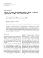
Figure 4: The 17 taps bandpass filter used as the linear channel in
the Wiener system, generated in Matlab as fir1(16,[0.25,0.75]).
two different nonlinearities were used. The exact setup is
specified in each experiment, and the length of the linear
filter is supposed to be known in all cases. In [22], it was
shown that the performance of the kernel CCA algorithm for
Wiener identification is hardly affected by overestimation of
the linear channel length. Therefore, if the exact filter length
was not known, it could be overestimated without significant
performance loss.
5.1. Batch identification
In the first experiment, we compare the performance of the
different constraints to minimize the error
r
x
− r
y

2
be-
tween the linear and nonlinear estimates in the simultaneous
identification scheme from Section 3. The identification of a
static Wiener system is treated here as a batch problem, that
is, all data points are available beforehand.
The Wiener system used for this setup consists of the
static linear channel from [10] representing an FIR bandpass

filter of 17 taps (see Figure 4) and a static nonlinearity given
by f (x)
= 0.2x +tanh(x). 500 samples are used to identify
this system.
To represent the inverse nonlinearity, a kernel expansion
is used, based on a Gaussian kernel with kernel size σ
= 0.2.
In order to avoid overfitting of the kernel matrix, L
2
regular-
ization is applied by adding a constant c
= 10
−4
to its diago-
nal.
Three different identification approaches are applied, us-
ing different constraints to minimize the error
e
2
. As dis-
cussed in Section 2, these constraints can be based on the fil-
ter coefficients or the signal energy. In a first approach, we
apply the filter coefficient norm constraint (2) (from [10]),
which fixes h
1
= 1. The corresponding optimal estimators
8 EURASIP Journal on Advances in Signal Processing
50403020100−10−20
SNR (dB)
h

1
= 1
h
2
+ α
2
= 1
r
x

2
=r
y

2
= 1
−40
−30
−20
−10
0
10
MSE (dB)
Figure 5: MSE e
r

2
on the Wiener system’s internal signal. The al-
gorithmsbasedonfiltercoefficient constraints (dotted and dashed
lines) perform worse than the proposed KCCA algorithm (solid

line), which is based on a signal power constraint.
are found by solving a simple LS problem. If, instead, we fix
the filter norm
h
2
+ α
2
= 1, we obtain the following
problem:
min


r
x
− r
y


2
s.t. h
2
+ α
2
= 1, (37)
which, after introducing the substitutions L
= [X, −K
y
]and
v
= [h

T
, α
T
]
T
,becomes
min
Lv
F
= min


v
T
L
T
Lv


s.t. v
2
= 1. (38)
The solution v of this second approach is found as the eigen-
vector corresponding to the smallest eigenvalue of the matrix
L
T
L. As a third approach, we apply the signal energy-based
constraint (3), which fixes
r
x


2
=r
y

2
= 1. The corre-
sponding solution is obtained by solving the GEV (21).
In Figure 5, the performance results are shown for the
three approaches and for different noise levels. To calculate
the error e
r
= r − r,bothr and r have been normalized
to compensate for the scaling indeterminacy of the Wiener
system. The MSE is obtained by averaging out
e
r

2
over
250 runs of the algorithms. As can be observed, the algo-
rithms based on the filter coefficient constraints perform
clearly worse than the proposed KCCA algorithm, which is
more robust to noise.
Figure 6 compares the real inverse nonlinearity to the es-
timate of this nonlinearity for the solution based on the h
1
fil-
ter coefficient constraint and to the estimate obtained by reg-
ularized KCCA. For 20 dB of output noise, the results of the

first algorithm are dominated by noise enhancement prob-
lems (Figure 6(d)). This further illustrates the advantage of
the signal power constraint over the filter coefficient con-
straint.
In the second experiment, we compare the full Wiener
system identification results for the KCCA approach to two
black box neural network methods, specifically a radial basis
function (RBF) network and a multilayer perceptron (MLP).
The Wiener system setup and used input signal are the same
as in the previous experiment.
For a fair comparison, the used solution methods should
have similar complexity. Since complexity comparison is dif-
ficult due to the significant architectural differences between
kernel and classic neural network approaches [15], we com-
pare the identification methods when simply given a similar
number of parameters. The KCCA algorithm requires 17 pa-
rameters to identify the linear channel and 500 parameters
in its kernel expansion, totalling 517. When the RBF network
and the MLP have 27 neurons in their hidden layer, they ob-
tain a comparable total of 514 parameters, considering they
use a time-delay input of length 17. For the MLP, however,
better results were obtained by lowering its number of neu-
rons, and therefore, we only assigned it 15 neurons. The RBF
network was trained with a sum-squared error goal of 10
−6
and the Gaussian function of its centers had a spread of 10.
TheMLPusedahyperbolictangenttransferfunction,and
it was trained over 50 epochs with the Levenberg-Marquardt
algorithm.
The results of the batch identification experiment can be

seen in Figure 7. The KCCA algorithm performs best due
to its knowledge of the internal structure of the system.
Note that by choosing the hyperbolic tangent function as the
transfer function, the MLP’s structure closely resembles the
used Wiener system and, therefore, also obtains good perfor-
mance.
5.2. Online identification
In a second set of simulations, we compare the identification
performance of the three adaptive kernel CCA-based identi-
fication algorithms from Section 4. In all online experiments,
the optimal parameters as well as the kernel for each of the
algorithms were determined by an exhaustive search.
5.2.1. Static Wiener system identification
The Wiener system used in this experiment contained the
same linear channel as in the previous batch example, fol-
lowed by the nonlinearity f (x)
= tanh(x). No output noise
was added in this first setup.
We applied the three proposed adaptive kernel CCA-
based algorithms with the following parameters:
(i) kernel CCA with standard regularization, c
= 10
−3
,
and a sliding window of 150 samples, using the Gaus-
sian kernel function with kernel width σ
= 0.2;
(ii) kernel CCA based on kernel PCA using 15 eigenvec-
tors calculated from a 150-sample sliding window, and
applying the polynomial kernel function of order 3;

(iii) kernel CCA with the dictionary-based sparsification
method from [28], with a polynomial kernel function
of order 3 and accuracy parameter ν
= 10
−4
.Thispa-
rameter controls the level of sparsity of the solution.
The RLS algorithm used in all three cases was a standard
exponentially weighted RLS algorithm [29] with a forgetting
factor of 0.99.
Steven Van Vaerenbergh et al. 9
0.20.10−0.1−0.2
−2
−1
0
1
2
(a) r[n] versus y[n],nonoise
210−1−2
−2
−1
0
1
2
(b) r[n] versus r[n], 20 dB SNR
0.20.10−0.1−0.2
−2
−1
0
1

2
(c) Estimate with h
1
constraint, no noise
0.20.10−0.1−0.2
−2
−1
0
1
2
(d) Estimate with h
1
constraint, 20 dB SNR
0.20.10−0.1−0.2
−2
−1
0
1
2
(e) KCCA estimate, no noise
0.20.10−0.1−0.2
−2
−1
0
1
2
(f) KCCA estimate, 20 dB SNR
Figure 6: Estimates of the nonlinearity in the static Wiener system. The top row shows the true signal r[n] versus the points y[n] representing
the system nonlinearity, for a noiseless case in (a) and a system that has 20 dB white Gaussian noise at its output in (b). The second and third
row show r

y
[n]versusy[n] obtained by applying the filter coefficient constraint h
1
= 1 and the signal power constraint (KCCA solution),
respectively.
The obtained MSE e
2
r
[n] for the three algorithms can be
seen in Figure 8. Most notable is the slow convergence of
the dictionary-based kernel CCA implementation. This is ex-
plained by the fact that the used dictionary-based kernel RLS
algorithm from [28] is lacking a forgetting mechanism and,
therefore, it takes a large number of iterations for the influ-
ence of the initially erroneous reference signal
r to decrease.
The kernel PCA-based algorithm obtains its optimal perfor-
mance for a polynomial kernel, while the L
2
regularized ker-
nel CCA algorithm performs slightly better, with the Gaus-
sian kernel.
A comparison of the results of the sliding window KCCA
algorithm for different noise levels is given in Figure 9. A dif-
ferent Wiener system was used, with linear channel H(z)
=
1+0.3668z
−1
− 0.5764z
−2

+0.2070z
−3
and nonlinearity
f (x)
= tanh(x).
10 EURASIP Journal on Advances in Signal Processing
50403020100−10−20
SNR (dB)
RBF network
MLP
KCCA
−40
−30
−20
−10
0
10
MSE (dB)
Figure 7: Full identification MSE e
y

2
of the Wiener system, using
two black box methods (RBF network and MLP) and the proposed
KCCA algorithm.
25002000150010005000
Iteration
Dictionary-based
Kernel-PCA
L

2
regularization
−40
−30
−20
−10
0
MSE (dB)
Figure 8: MSE e
2
r
[n] on the Wiener system’s internal signal r[n]
for adaptive kernel CCA-based identification of a static noiseless
Wiener system.
25002000150010005000
Iteration
SNR
= 10dB
SNR
= 20dB
SNR
= 40dB
−30
−20
−10
0
10
MSE (dB)
Figure 9: MSE e
2

r
[n] on the Wiener system’s internal signal r[n]for
various noise levels, obtained by the adaptive KCCA algorithm.
Figure 10 shows the full system identification results ob-
tained by an MLP and the proposed KCCA algorithm on this
wiener system. The used MLP has learning rate 0.01 and was
25002000150010005000
Iteration
MLP
KCCA
−25
−20
−15
−10
−5
0
5
MSE (dB)
Figure 10: MSE e
2
y
[n] for full system identification of the Wiener
system, using a black-box method (MLP) and the proposed KCCA
algorithm.
trained at each iteration step with the new data point. The
KCCA algorithm again has L
2
regularization with c = 10
−3
,

σ
= 0.2, and a sliding window of 150 samples. Both the in-
verse nonlinearity and the direct nonlinearity were estimated
with the sliding-window kernel RLS technique. Although this
algorithm converges slower, it is clear that its knowledge of
the internal structure of the Wiener system implies a consid-
erable advantage over the black-box approach.
5.2.2. Dynamic Wiener system identification
In a second experiment, the tracking capabilities of the dis-
cussed algorithms were tested. Therefore, an abrupt change
in the Wiener system was triggered (note that although only
the linear filter is changed, the proposed adaptive identifica-
tion method allows both parts of the Wiener system to be
varying in time): during the first part, the Wiener system
uses the 17-coefficient channel from the previous tests, but
after receiving the 1000th data point, its channel is changed
to H(z)
= 1+0.3668z
−1
− 0.5764z
−2
+0.2070z
−3
. The non-
linearity was f (x)
= tanh(x) in both cases. Moreover, 20 dB
of zero-mean white Gaussian noise was added to the output
of the system during the entire experiment.
The parameters of the applied identification algorithms
were chosen as follows.

(i) For Kernel CCA with standard regularization, we used
c
= 10
−3
, a sliding window of 150 samples, and the
polynomial kernel function of order 3.
(ii) The Kernel CCA algorithm based on kernel PCA was
used with 15 eigenvectors, a sliding window of 150
samples, and the polynomial kernel function of or-
der 3.
(iii) Finally, for Kernel CCA with the dictionary-based
sparsification method, we used accuracy parameter
ν
= 10
−3
and a polynomial kernel function of order 3.
The length of the estimated linear channel was fixed as 17
during this experiment, resulting in an overestimated chan-
nel estimate in the second part.
Steven Van Vaerenbergh et al. 11
25002000150010005000
Iteration
Dictionary-based
Kernel-PCA
L
2
regularization
−25
−20
−15

−10
−5
0
MSE (dB)
Figure 11: Wiener system MSE e
2
r
[n] obtained by adaptive iden-
tification of a Wiener system that exhibits an abrupt change and
contains additive noise.
The identification results can be seen in Figure 11.Asin
the case of the static Wiener system, the dictionary-based
kernel CCA algorithm obtains the worst performance, for
reasons discussed earlier. The algorithm based on standard
regularization and the one based on kernel PCA obtain very
similar performance.
5.2.3. Static Hammerstein system identification
In this setup, we considered a static Hammerstein system
consisting of the nonlinearity f (x)
= tanh(x) followed by the
linear channel H(z)
= 1 − 0.4326
−1
+0.3656z
−2
− 0.3153z
−3
.
To the output of this system, 20 dB zero-mean additive white
Gaussian noise was added. When applying the proposed ker-

nel CCA-based algorithms to identify this system, the direct
nonlinearity is estimated and an FIR estimate is made of the
inverse linear channel which corresponds to an IIR filter. To
adequately estimate this channel, the length of the direct FIR
filter estimate was considerably increased.
The adaptive kernel CCA algorithms were applied with
the following parameters:
(i) kernel CCA with standard regularization, c
= 10
−2
,
and a sliding window of 150 samples, using the Gaus-
sian kernel function with kernel width σ
= 0.2;
(ii) kernel CCA based on kernel PCA using 10 eigenvec-
tors, a 150-sample sliding window and the Gaussian
kernel function with kernel width σ
= 0.2;
(iii) kernel CCA with dictionary-based sparsification, us-
ing accuracy parameter ν
= 10
−2
and the same Gaus-
sian kernel function.
In all three algorithms, the inverse linear channel was ap-
proximated as an FIR channel of length 15.
The MSE results for the Hammerstein system identifica-
tion can be found in Figure 12. The observed MSE perfor-
mances are similar to the observations already made for the
previous examples. However, due to the different setup and

the presence of noise, the obtained results are not as good as
those of the identification of a static noiseless Wiener system
(see Figure 8). Nevertheless, with the chosen parameters, the
25002000150010005000
Iteration
Dictionary-based
Kernel-PCA
L
2
regularization
−20
−15
−10
−5
0
MSE (dB)
Figure 12: MSE e
2
r
[n] on the Hammerstein system’s internal signal
r[n] for the three adaptive kernel CCA-based algorithms.
L
2
regularization-based kernel CCA algorithm is capable of
attaining the 20 dB noise floor.
In all previous examples, the length N
w
of the sliding
windows for the L
2

regularization-based kernel CCA and
the kernel PCA-based kernel CCA was fixed as 150. Taking
into account the number of eigenvectors used by the latter,
both obtain a very similar computational complexity. The
dictionary-based algorithm, on the other hand, is computa-
tionally much more attractive with its O(M
2
) complexity, but
it is not capable of obtaining the same performance levels.
6. CONCLUSIONS AND DISCUSSION
In this paper, we have proposed a kernel-CCA-based frame-
work to simultaneously identify the two parts of a Wiener or
a Hammerstein system. Applying the correct restrictions on
the solutions, it was shown how the proposed kernel CCA
algorithm emerges as the logical solution to identify these
nonlinear systems. Three different approaches to regularize
the solutions of this kernel algorithm were discussed, result-
ing in three different implementations. In the second part of
this paper, we showed how adaptive versions of these three
algorithms could be derived, based on existing kernel RLS
implementations and the reformulation of kernel CCA as a
set of LS regression problems.
The proposed algorithms were compared in a series of
batch and online experiments. The kernel CCA algorithm
using the dictionary-based kernel RLS from [28]wasfound
not suitable for adaptive kernel CCA since it is incapable of
efficiently performing tracking. The kernel CCA algorithm
using L
2
regularization and a sliding window obtained simi-

lar performance and computational cost as the kernel-PCA-
based algorithm. These two algorithms showed to be success-
ful in identifying both static and time-varying Wiener and
Hammerstein systems.
Many directions for future research are open. The pro-
posed methods can be used directly in problems with com-
plex signals, such as communication signals, for instance, in
the identification of nonlinear power amplifiers for OFDM
systems [37]. Another possibility to explore is the application
12 EURASIP Journal on Advances in Signal Processing
of kernel CCA to more complex cascade models such as the
three-block Wiener-Hammerstein systems. And lastly, the
problem of extending the proposed algorithms to blind iden-
tification can be considered.
ACKNOWLEDGMENTS
This work was supported by MEC (Ministerio de Educaci
´
on
y Ciencia, Spain) under Grants no. TEC2004-06451-C05-02,
TEC2007-68020-C04-02 TCM, and FPU Grant no. AP2005-
5366.
REFERENCES
[1] G. Giannakis and E. Serpedin, “A bibliography on nonlin-
ear system identification,” Signal Processing,vol.81,no.3,pp.
533–580, 2001.
[2] O. Nelles, Nonlinear System Identification, Springer, Berlin,
Germany, 2000.
[3] G. Kechriotis, E. Zervas, and E. S. Manolakos, “Using recur-
rent neural networks for adaptive communication channel
equalization,” IEEE Transactions on Neural Networks, vol. 5,

no. 2, pp. 267–278, 1994.
[4] N. P. Sands and J. M. Cioffi, “Nonlinear channel models for
digital magnetic recording,” IEEE Transactions on Magnetics,
vol. 29, no. 6, pp. 3996–3998, 1993.
[5] A. Balestrino, A. Landi, M. Ould-Zmirli, and L. Sani, “Auto-
matic nonlinear auto-tuning method for Hammerstein mod-
eling of electrical drives,” IEEE Transactions on Industrial Elec-
tronics, vol. 48, no. 3, pp. 645–655, 2001.
[6] D. Erdogmus, D. Rende, J. C. Principe, and T. F. Wong,
“Nonlinear channel equalization using multilayer percep-
trons with information-theoretic criterion,” in Proceedings of
the IEEE Workshop on Neural Networks for Signal Processing
XI (NNSP ’01), pp. 443–451, North Falmouth, Mass, USA,
September 2001.
[7] T. Adali and X. Liu, “Canonical piecewise linear network for
nonlinear filtering and its application to blind equalization,”
Signal Processing, vol. 61, no. 2, pp. 145–155, 1997.
[8] M. Pawlak, Z. Hasiewicz, and P. Wachel, “On nonparametric
identification of Wiener systems,” IEEE Transactions on Signal
Processing, vol. 55, no. 2, pp. 482–492, 2007.
[9] J. Wang, A. Sano, T. Chen, and B. Huang, “Blind Hammerstein
identification for MR damper modeling,” in Proceedings of the
American Control Conference (ACC ’07), pp. 2277–2282, New
York, NY, USA, July 2007.
[10] E. Aschbacher and M. Rupp, “Robustness analysis of a gra-
dient identification method for a nonlinear wiener system,” in
Proceedings of the 13th IEEE Workshop on Statistical Signal Pro-
cessing (SSP ’05), vol. 2005, pp. 103–108, Bordeaux, France,
July 2005.
[11] D. T. Westwick and R. E. Kearney, “Identification of a Ham-

merstein model of the stretch reflex EMG using separable least
squares,” in Proceedings of the 22nd Annual International Con-
ference of the IEEE Engineering in Medicine and Biology Soci-
ety (IEMBS ’00), vol. 3, pp. 1901–1904, Chicago, Ill, USA, July
2000.
[12] J. E. Cousseau, J. L. Figueroa, S. Werner, and T. I. Laakso, “Effi-
cient nonlinear Wiener model identification using a complex-
valued simplicial canonical piecewise linear filter,” IEEE Trans-
actions on Signal Processing, vol. 55, no. 5, pp. 1780–1792,
2007.
[13] A. Taleb, J. Sole, and C. Jutten, “Quasi-nonparametric blind
inversion of Wiener systems,” IEEE Transactions on Signal Pro-
cessing, vol. 49, no. 5, pp. 917–924, 2001.
[14] J. C. Gomez and E. Baeyens, “Subspace-based blind identifi-
cation of IIR Wiener systems,” in Proceedings of 15th European
Signal Processing Conference (EUSIPCO ’07),Pozna
´
n, Poland,
September 2007.
[15] B. Sch
¨
olkopf and A. J. Smola, Learning with Kernels, MIT Press,
Cambridge, Mass, USA, 2002.
[16] S. Haykin, Neural Networks: A Comprehensive Foundation,
Prentice-Hall, Englewood Cliffs, NJ, USA, 2nd edition, 1999.
[17] G. S. Kimeldorf and G. Wahba, “Some results on Tchebychef-
fian spline functions,” Journal of Mathematical Analysis and
Applications, vol. 33, no. 1, pp. 82–95, 1971.
[18] F. R. Bach and M. I. Jordan, “Kernel independent component
analysis,” Journal of Machine Learning Research, vol. 3, pp. 1–

48, 2003.
[19] D. R. Hardoon, S. Szedmak, and J. Shawe-Taylor, “Canonical
correlation analysis: an overview with application to learning
methods,” Tech. Rep. CSD-TR-03-02, Royal Holloway, Univer-
sity of London, Egham, Surrey, UK, 2003.
[20] P. L. Lai and C. Fyfe, “Kernel and nonlinear canonical correla-
tion analysis,” International Journal of Neural Systems, vol. 10,
no. 5, pp. 365–377, 2000.
[21] H. Hotelling, “Relations between two sets of variates,”
Biometrika, vol. 28, pp. 321–377, 1936.
[22] S. Van Vaerenbergh, J. V
´
ıa, and I. Santamar
´
ıa, “Online kernel
canonical correlation analysis for supervised equalization of
Wiener systems,” in Proceedings of the International Joint Con-
ference on Neural Networks (IJCNN ’06), pp. 1198–1204, Van-
couver, BC, Canada, July 2006.
[23] J. V
´
ıa, I. Santamar
´
ıa, and J. P
´
erez, “Canonical correlation anal-
ysis (CCA) algorithms for multiple data sets: application to
blind SIMO equalization,” in Proceedings of the 13th European
Signal Processing Conference (EUSIPCO ’05), Antalya, Turky,
September 2005.

[24] A. Tikhonov, “Solution of incorrectly formulated problems
and the regularization method,” Soviet Mathematics Doklady,
vol. 4, pp. 1035–1038, 1963.
[25] S. Van Vaerenbergh, J. V
´
ıa, and I. Santamar
´
ıa, “A sliding-
window kernel RLS algorithm and its application to nonlinear
channel identification,” in Proceedings of the IEEE International
Conference on Acoustics, Speech and Signal Processing (ICASSP
’06), vol. 5, pp. V789–V792, Toulouse, France, May 2006.
[26] K. I. Diamantaras and S. Y. Kung, Principal Component Neural
Networks: Theory and Applications, John Wiley & Sons, New
York, NY, USA, 1996.
[27] B. Sch
¨
olkopf, A. Smola, and K R. M
¨
uller, “Nonlinear compo-
nent analysis as a kernel eigenvalue problem,” Neural Compu-
tation, vol. 10, no. 5, pp. 1299–1319, 1998.
[28] Y. Engel, S. Mannor, and R. Meir, “The kernel recursive least
squares algorithm,” IEEE Transactions on Signal Processing,
vol. 52, no. 8, pp. 2275–2285, 2004.
[29] S. Haykin, Adaptive Filter Theory, Prentice-Hall, Englewood
Cliffs, NJ, USA, 4th edition, 2001.
[30] J. V
´
ıa, I. Santamar

´
ıa, and J. P
´
erez, “A learning algorithm for
adaptive canonical correlation analysis of several data sets,”
Neural Networks, vol. 20, no. 1, pp. 139–152, 2007.
[31] A. Pezeshki, L. L. Scharf, M. R. Azimi-Sadjadi, and Y. Hua,
“Two-channel constrained least squares problems: solutions
using power methods and connections with canonical coor-
dinates,” IEEE Transactions on Signal Processing, vol. 53, no. 1,
pp. 121–135, 2005.
Steven Van Vaerenbergh et al. 13
[32] J. V
´
ıa, I. Santamar
´
ıa, and J. P
´
erez, “A robust RLS algorithm for
adaptive canonical correlation analysis,” in Proceedings of the
IEEE International Conference on Acoustics, Speech and Signal
Processing (ICASSP ’05), vol. 4, pp. 365–368, Philadelphia, Pa,
USA, March 2005.
[33] J. Kivinen, A. J. Smola, and R. C. Williamson, “Online learning
with kernels,” IEEE Transactions on Signal Processing, vol. 52,
no. 8, pp. 2165–2176, 2004.
[34] S. Van Vaerenbergh, J. V
´
ıa, and I. Santamar
´

ıa, “Nonlinear sys-
tem identification using a new sliding-window kernel RLS al-
gorithm,” Journal of Communications, vol. 2, no. 3, pp. 1–8,
2007.
[35] L. Hoegaerts, L. De Lathauwer, I. Goethals, J. A. K. Suykens, J.
Vandewalle, and B. De Moor, “Efficiently updating and track-
ing the dominant kernel principal components,” Neural Net-
works, vol. 20, no. 2, pp. 220–229, 2007.
[36] E. Andeli
´
c, M. Schaff
¨
oner, M. Katz, S. E. Kr
¨
uger, and A. Wen-
demuth, “Kernel least-squares models using updates of the
pseudoinverse,” Neural Computation, vol. 18, no. 12, pp. 2928–
2935, 2006.
[37] I. Santamar
´
ıa, J. Ib
´
a
˜
nez, M. L
´
azaro, C. Pantale
´
on, and L.
Vielva, “Modeling nonlinear power amplifiers in OFDM sys-

tems form subsampled data: a comparative study using real
measurements,” EURASIP Journal on Applied Signal Process-
ing, vol. 2003, no. 12, pp. 1219–1228, 2003.