Báo cáo hóa học: " Research Article Joint Throughput Maximization and Fair Uplink Transmission Scheduling in CDMA Systems" potx

Hindawi Publishing Corporation
EURASIP Journal on Wireless Communications and Networking
Volume 2009, Article ID 564692, 15 pages
doi:10.1155/2009/564692

Research Article
Joint Throughput Maximization and Fair Uplink Transmission
Scheduling in CDMA Systems
Symeon Papavassiliou1, 2 and Chengzhou Li3
1 Network

Management and Optimal Design Laboratory (NETMODE), Institute of Communications and Computer Systems (ICCS),
9 Iroon Polytechniou Street, Zografou 157 73, Athens, Greece
2 School of Electrical and Computer Engineering, National Technical University of Athens (NTUA), 9 Iroon Polytechniou Street,
Zografou 157 73, Athens, Greece
3 LSI Corporation, 1110 American Parkway NE, Allentown, PA 18109, USA
Correspondence should be addressed to Symeon Papavassiliou,
Received 9 July 2008; Revised 10 December 2008; Accepted 20 February 2009
Recommended by Alagan Anpalagan
We study the fundamental problem of optimal transmission scheduling in a code-division multiple-access wireless system in order
to maximize the uplink system throughput, while satisfying the users quality-of-service (QoS) requirements and maintaining
fairness among them. The corresponding problem is expressed as a weighted throughput maximization problem, under certain
power and QoS constraints, where the weights are the control parameters reflecting the fairness constraints. With the introduction
of the power index capacity, it is shown that this optimization problem can be converted into a binary knapsack problem, where all
the corresponding constraints are replaced by the power index capacities at some certain system power index. A two-step approach
is followed to obtain the optimal solution. First, a simple method is proposed to find the optimal set of users to receive service for
a given fixed target system load, and then the optimal solution is obtained as a global search within a certain range. Furthermore, a
stochastic approximation method is presented to effectively identify the required control parameters. The performance evaluation
reveals the advantages of our proposed policy over other existing ones and confirms that it achieves very high throughput while
maintains fairness among the users, under different channel conditions and requirements.
Copyright © 2009 S. Papavassiliou and C. Li. This is an open access article distributed under the Creative Commons Attribution

License, which permits unrestricted use, distribution, and reproduction in any medium, provided the original work is properly
cited.

1. Introduction
The continuous growth in traffic volume and the emergence
of new services have begun to change the structure and
requirements of wireless networks. Future mobile communication systems will be characterized by high throughput,
integration of services, and flexibility [1–5]. With the
demand for high data rate and support of multiple quality of
service (QoS), the transmission scheduling plays a key role in
the efficient resource allocation process in wireless systems.
The transmission scheduling determines the time instances
that a mobile user may receive service, as well as the resources
that should be allocated to support the requested service, in
order to make the resource distribution fair and efficient.
The fundamental problem of scheduling the users transmission and allocating the available resources in a realistic uplink code-division multiple-access (CDMA) wireless

system that supports multirate multimedia services, with
efficiency and fairness, is investigated and analyzed in this
paper. A transmission scheduling method which achieves
the maximum system throughput under the constraints
of satisfying certain users QoS requirements and maintaining throughput fairness among them is provided and
evaluated.
1.1. Related Work and Motivation. A class of scheduling
schemes, namely, the opportunistic scheduling schemes,
has been proven to be an effective approach to improve
the system throughput by utilizing the multiuser diversity
effect [6, 7] in wireless communications. Specifically, for
a system with many users that have independent varying
channels, with high probability there is a user with channel

much stronger than its average SNR requirement. Therefore,
the system throughput may be maximized by choosing


2

EURASIP Journal on Wireless Communications and Networking

the user with “relatively best” channel for transmission at
a given slot. However, some fairness constraints must be
imposed on the scheduling policies to ensure the fair resource
allocation.
It has been shown in [8] that scheduling users one-byone can result in higher system throughput for high data
rate traffic in the CDMA downlink. However, this work
does not exploit the time-varying channel conditions. In
[7, 9], a high-speed data rate scheme (HDR) is introduced,
where the base station schedules the downlink transmission
of a single user at a given time slot with the data rates
and slot lengths varying according to the specific channel
condition. In [10–12], a transmission scheduling scheme for
multiple users, which considers both the channel condition
and queueing delay/length, is proposed and shown to be
throughput optimal if it is feasible. However, the fairness
issue is not explicitly addressed in that work. In [13–15],
a framework for opportunistic scheduling that maximizes
the system performance by exploiting the time-varying
channel conditions of wireless networks is presented. Three
categories of scheduling problems—the temporal fairness,
utilitarian fairness, and minimum-performance guarantee
scheduling—are studied and optimal solutions are given.

Although the downlink transmission assignment is
important for several applications, the efficient uplink
transmission scheduling plays an important role as well,
especially with the prevailing of multimedia communications and applications. It has been argued that the downlink
scheduling method is not suitable to be applied to the uplink
transmission scheduling, where simultaneous transmissions
may result in higher throughput [16, 17]. The uplink
transmission scheduling problem is more complicated and
requires further consideration of additional elements to
make the corresponding scheduling policies feasible [18].
The achievable throughput in such a case depends not only
on the service access time, but also on the transmission powers and the corresponding users interference. In addition,
multiple users can be scheduled simultaneously to transmit
in the same time slot, which is a major difference from
the wireline and TDMA-like scheduling schemes, making
the respective scheduling processes either inapplicable or
inefficient in the CDMA environment. The simple temporal
fairness scheduling, where the main resource to be shared is
the time, fails to provide rational fairness in this case. As a
result, the throughput optimal and fair uplink transmission
scheduling problem needs to jointly consider multiple factors
such as access time, transmission power, channel conditions,
and number of users to be scheduled at the same time.
Heuristic approaches to address the problem of short-term
fairness and demonstrate the tradeoff between fairness and
throughput under some special cases have been introduced
in [19–21].
Furthermore, how to maximize the throughput of uplink
CDMA system was first analyzed in [16]. The sole purpose
of uplink throughput maximization can be achieved by

choosing the “best” K users in terms of their received power,
when they transmit at their maximum power. However, such
throughput maximization does not consider fairness, that is,
the equal opportunity for all users to receiving service despite

their channel conditions. Therefore, among the objectives
of our approach in this paper is to identify the actual
“best” users that should transmit in order to maximize the
throughput, when the fairness constraints are introduced
and respected.
In [22], several scenarios of scheduling uplink CDMA
transmission with voice and data services are analyzed.
With the number of voice users and their corresponding
transmission rates fixed, that work attempted to maximize
the throughput of data service. It was shown that when the
synchronization overhead is reasonable, a smaller number
of simultaneous transmission users achieve higher system
throughput and at the same time lower the average transmission power. However, in this case the achievable throughput
is affected by the “weakest link.” Therefore, this approach
can be regarded only as a static analysis that considers the
relationship between the performance and the number of
users chosen for transmission. The problem of identifying
the actual set of users to transmit based on their channel
conditions, which may reduce the impact of the “weakest
link”, has not yet been investigated and is one of the main
objectives of our paper.
In addition, the problem of uplink CDMA scheduling is
further complicated by the fact that the conventional concept
of capacity used in the wireline networks, for example, total
bandwidth of the physical media, is not directly applicable in

the CDMA systems. In this case, the actual system capacity
is not fixed and known in advance, since it is a function of
several parameters such as the number of users, the channel
conditions, and the transmission powers.
Therefore, in summary the main contributions of this
paper are as follows. (1) Jointly consider the factors of
channel capacity, number of users and their interference,
transmit power, and fairness requirements. (2) Formulate an
optimization problem that stresses the fairness requirement
under time-varying wireless environment and proves the
existence of an optimal solution based on all constraints. (3)
Exploit the power index concept and power index capacity,
as a novel and effective way, to treat the fairness issue in
the transmission scheduling policy under the considered
uncertain and dynamic environment. (4) Devise a scheduling
policy that achieves throughput fairness among the users and
optimal system throughput under certain constraints.
1.2. Paper Outline. The rest of the paper is organized
as follows. In Section 2, the system model that is used
throughout our analysis is described, and the problem
of the uplink scheduling in CDMA systems is rigorously
formulated as a multiconstraint optimization problem. It
is demonstrated that this problem can be expressed as a
weighted throughput maximization problem, under certain
power and QoS constraints, where the weights are the
control parameters that reflect fairness constraints. Based
on the concept of power index capacity, this optimization
problem is converted into a simpler linear knapsack problem
in Section 3.1, where all the corresponding constraints are
replaced by the users power index capacities at some

certain system power index. The optimal solution of the
latter problem is identified in Sections 3.2 and 3.3, while


EURASIP Journal on Wireless Communications and Networking
in Section 3.4, a stochastic approximation method is presented in order to effectively identify the required control
parameters. Section 4 contains the performance evaluation
of the proposed method, along with some numerical
results and discussion, and finally Section 5 concludes the
paper.

3

subject to specific SINR, maximum transmit power, and
fairness constraints as follows:
h i p i Gi
B(k)
j =1, j = i
/

rj
ri
=
φi
φj

In this paper, we consider a single cell DS-CDMA system
with B(k) backlogged users at time slot k. The users
channel conditions are assumed to change according to some
stationary stochastic process, while the uplink transmission

rate is assumed to be adjustable with the variable spreading
gain technique [23]. Each user i is associated with some
preassigned weight φi according to its QoS requirement. In
the following for simplicity in the presentation, we omit
the notation of the specific slot k from the notations and
definitions we introduce. Let us denote by ri the transmission
rate of user i in the slot under consideration. We assume
that the chip rate W for all mobiles is fixed, and hence the
spreading gain Gi of user i is defined as Gi = W/ri . Let
us also denote by γi the required signal-to-interference and
noise ratio (SINR) level of user i, by hi the corresponding
channel gain, and by pi the user i transmission power at a
given slot, which, however, is limited by the maximum power
value pimax . Therefore, the received SINR γi for a user i is
given by

α

+ Wη0

= γi ,

i = 1, 2, . . . , B(k),

(1)

≥ γi ,

for i = 1, 2, . . . , B(k),

pi ≤ pimax , for i = 1, 2, . . . , B(k),

2. System Model and Problem Formulation

h i p i Gi
B(k)
j =1, j = i h j p j
/

h j p j + Wη0

(3)

for 1 ≤ i, j ≤ B(k),

where r i = E(ri ) denotes the mean throughput of user i in
the corresponding backlogged period. It has been shown in
[15, 24] that the above-constrained optimization problem
can be considered as equivalent to the following problem
(4), where Z is the minimal value among all r i /φi , that is,
Z = mini {r i /φi }. In (4), we transform the objective function
(2) into finding the optimal transmit powers and rates that
maximize the minimal normalized average rate Z. Therefore,
max Z,
ri
s.t. Z ≤ , 1 ≤ i ≤ B(k),
φi
hi pi W/ri
≥ γi i = 1, 2, . . . , B(k),
B(k)

j =1, j = i h j p j + Wη0
/
pi ≤ pimax ,

(4)

1 ≤ i ≤ B(k).

Apparently, the solution of the above problem will finally
make Z = r i /φi for 1 ≤ i ≤ B(k) since one can always
reduce its throughput for the benefit of other users in order
to maximize Z. With the constraint Z = r i /φi , the objective
function then is generalized to
B(k)

where η0 is the one-sided power spectral density of additive
white Gaussian noise (AWGN), and α determines the
proportion of the interference from other users received
power. Without loss of generality in the following, we assume
α = 1. Obviously, to meet the SINR requirement, the received
SINR γi has to be larger than the corresponding threshold
γi , that is, γi ≥ γi . In the following, we assume perfect
power control in the system under consideration, while
users are scheduled to transmit at the beginning of every
fixed-length slot. The objective of the optimal scheduling
policy Q∗ is to find the optimal number of allowable
users and their transmission rates, which achieves the
maximum system throughput while maintaining the fairness
property.
B(k)

2.1. Problem Formulation. Let R(k) =
i=1 ri (k) denote
the total throughput in slot k. Our objective function is to
maximize the expectation of R(k) by selecting the optimal
transmit power vector (p1 , p2 , . . . , pB(k) ) and transmit rate
vector (r1 , r2 , . . . , rB(k) ), that is,

B(k)

max E

ri
i=1

(2)

wi r i ,

max

(5)

i=1

where wi is an arbitrary positive number. Here the crucial
observation [24] is that the optimal scheduling policy will be
the one that maximizes the sum of weighted throughputs and
equalizes the normalized throughput. The maximization of
mean-weighted rate in (5) is obtained by the maximization
of the weighted rate in every slot, that is, max iB(k) wi ri

=1
for every slot k. In conclusion, to obtain the optimal
uplink throughput while keeping fairness, we must solve the
following problem:
B(k)

wi ri ,

max

(6)

i=1

s.t.

hi pi W/ri
B(k)
j =1, j = i h j p j + Wη0
/
pi ≤ pimax ,

≥ γi ,

i = 1, 2, . . . , B(k),

1 ≤ i ≤ B(k).

(7)
(8)

The fairness constraint, that is, r i /φi = r j /φ j , is
represented by the choice of wi . By adjusting the value of
wi , the user will get more or less opportunities to transmit
data, and hence the corresponding normalized throughput is
balanced. As we discuss later in this paper, the value of wi can


4

EURASIP Journal on Wireless Communications and Networking

be approximated by a stochastic approximation algorithm,
which has already found its application in [14, 15] under
similar situations. Note that since we assume perfect power
control in the CDMA system under consideration, only the
equality case of (7) is considered here.
The following Proposition 1 states that the optimal
solution is achieved when a user either transmits at full power
or does not transmit at all.
Proposition 1. The optimal solution that maximizes the
weighted throughput of problem (6) is such that
pi (k) ∈ 0, pimax ,

for i = 1, 2, . . . , B(k).

(9)

Proof. In order to minimize the multiple access interference,
users transmit with the minimum required power to meet

the required threshold γi . Therefore, we consider the equality
case of constraint (7). To maintain exactly the threshold γi for
user i, the achievable transmit rate is represented as
ri (k) =

γi

hi p i W
B(k)
j =1, j = i h j p j
/

+ Wη0

.

(10)

The objective function then becomes
B(k)

Z=

B(k)

wi ri =
i=1

wi hi W
γi

i=1

pi
B(k)
j =1, j = i
/

h j p j + Wη0

.

(11)

Differentiating twice with respect to the transmit power
of a user m, we obtain
B(k)

∂2 Z
wi hi W
=2
2
∂pm
γi
i=1,i = m
/

p i h2
m
B(k)
j =1, j = i

/

h j p j + Wη0

3.

In Section 3, the corresponding optimization problem
is transformed to an equivalent problem of a simpler
form, which facilitates the identification of the optimal
solution. However, in the following we first introduce
the concept of power index capacity which is used to
represent the corresponding constraints, under the problem
transformation.
2.2. Power Index Capacity. It has been shown in [25] that by
solving the constraints (7) and (8), the following inequality
must be satisfied if there exists a feasible power assignment
p = [p1 , p2 , . . . , pB(k) ] that meets the QoS requirements:
gi ≤ 1 −
i=1

η0 W
min1≤i≤B(k) pimax hi Gi /γi + 1

η0 W
=1−
,
min1≤i≤B(k) pimax hi /gi

gi =

γi
γ i + Gi

(14)

is defined as the power index of user i [26]. Relation
(13) is the necessary and sufficient condition such that a
power and rate solution is feasible under constraints (7) and
(8) [25].
Let us regard i gi as the actual system load, which is the
sum of power indices assigned to all backlogged users, while
we assume that there is a target system load ψ. It should be
noted that ψ here is not fixed but has value 0 ≤ ψ < 1.
The meaning and motivation for the definition of the target
system load ψ are that the system will attempt to provide the
appropriate scheduling in order to make the actual system
load gi reach the target load (however, it serves as an upper
bound and cannot be exceeded). For an arbitrarily selected
ψ in the range of 0 < ψ < 1, there exist two possible cases
concerning the relationship between the actual system load
gi and the target system load. When considering small
values for the target system load ψ, the system can easily
make the actual system load gi reach the target load under
consideration, that is, gi = ψ. On the other hand, when
ψ is large, especially when it approaches to 1, it may be
impossible for the actual achievable system load gi to reach
ψ due to the limitation imposed by (13). Let us assume that
in time slot k the maximum system load this system can
achieve based on all users channel states and all possible
user schedulings is ψ ∗ = max( gi ). We will now consider

the two cases mentioned above, that is, 0 < ψ ≤ ψ ∗ and
ψ > ψ ∗.

(12)

Since wi is positive number, obviously (12) is nonnegative,
while the objective function is a convex function of pm .
Hence, the optimal solution of this problem is that the
transmit power obtains the value of its boundary, that is,
either 0 or pimax .

B(k)

where

(13)

2.2.1. Target Load Is Less than or Equal to Maximum System
Load. If we assume 0 < ψ ≤ ψ ∗ , then the system load can
achieve the target load, i gi = ψ. Therefore, (13) can be
rewritten as follows:
min

1≤i≤B(k)

pimax hi
gi

≥

η0 W
,
1−ψ

gi ≤ ψ,
(15)

η0 W
pmax hi
therefore i
≥
gi
1−ψ

∀i, 1 ≤ i ≤ B(k).

For each individual user, there is a limitation on the
maximum power index that it can reach, given by (15)
gi ≤ (1 − ψ)

pimax hi
,
η0 W

gi ≤ ψ.

(16)

2.2.2. Target Load Is Larger than Maximum System Load. If
the target load is larger than the maximum system load, that

is, ψ > ψ ∗ , it means there will be no feasible transmission
power solution in (7) and (8) to achieve this target load and
therefore the relationship in (15) does not hold any more.
In this case, we simply apply the power index restriction of
(16) to each user. The consequence is that the final achieved
system load becomes i gi < ψ ∗ < ψ since gi ≤ (1 −
ψ)pimax hi /η0 W < (1 − ψ ∗ )pimax hi /η0 W.


EURASIP Journal on Wireless Communications and Networking
In fact, unless all possible transmission user sets are
searched, it is unknown in advance whether or not the actual
system load gi can reach the chosen ψ. Therefore, applying
(16) to the case ψ > ψ ∗ unifies the definition of the power
index range, within which a user can be assigned a feasible
power index without knowing the value of ψ ∗ . One key
principle and rule regarding the algorithm proposed in this
paper is to assign to an individual user a power index that is
less than or equal to its power index capacity. In the power
index assignment algorithm described in Section 3.2, the
situation where gi < ψ may occur. However, it should be
noted here that as proven by Theorem 1 later in the paper, the
global optimal solution must be the one satisfying gi = ψ.
The target load range where ψ > ψ ∗ is then not possible
to be the optimal solution. The intentionally introduced
restriction of (16) in the case of ψ > ψ ∗ allows the algorithm
to rule out such values of ψ due to the fact that gi < ψ in
this case.

5

3. Problem Transformation and
Optimal Solution
3.1. Problem Transformation. The corresponding constraints
in terms of the power index can be represented as follows:
B(k)

max Z =

w i f r gi , γ i ,

B(k)

gi ≤ ψ,

Definition 1. In a CDMA system with B(k) backlogged users
at time slot k, given the target system power index ψ, the
maximum power index that does not violate (13) for a single
user whose channel gain is hi is defined as the power index
capacity (PIC) πi (hi , ψ) of this user.
From (15), it can be easily found that the PIC of user i is

πi hi , ψ = min (1 − ψ)

pimax hi
,ψ .
η0 W

(17)

Note that in (17) the power index capacity is limited by the
target system power index. This is reasonable since a power
index capacity that is greater than ψ will have no practical
meaning and application. Furthermore, since our focus in
this paper is to find an optimal scheduling policy as well
as the optimal system load ψ, the value of ψ in (17) is not
determined in advance.
Intuitively, the power index represents the relationship
between the transmission power and the corresponding
interference that is caused to other users. If we considered
that the total system power index is fixed to ψ, larger
power index gi for user i indicates that it has relatively
higher signal-to-interference ratio compared to the other
users with smaller power index, while at the same time it
causes more interference to them. Accordingly, users with
high-power indices may lower their transmission power to
reduce the interference they may cause, which in turn means
that they will have smaller power index to limit the intracell
interference of the system, and therefore satisfy (13) that
guarantees the existence of a feasible transmission power
solution.

(19)

i=1

gi ≤ πi (hi , ψ),

1 ≤ i ≤ B(k),

0 ≤ ψ < 1.

(20)
(21)

Note that in the objective function we represent the rate
ri = fr (gi , γi ) as a function of power index gi , where
f r gi , γ i =

2.2.3. Definition of Power Index Capacity. Hence, given the
system load ψ the maximum possible power index gi a user
can accept in (15) is determined by the maximum transmit
power pimax and the channel gain hi .

(18)

i=1

gi

W
,
1 − gi γ i

(22)

which converts the power index into transmission rate and
can be easily derived from (14) by replacing Gi with W/ri .
In the following, let V = {v1 , v2 , . . . , vi , . . .} denote
the set that contains all the power and rate vectors that satisfy constraints (7) and (8) and vi =

{ p1,i , p2,i , . . . , pB(k),i , r1,i, r2,i , . . . , rB(k),i }. The elements p j,i and
r j,i represent the transmit power and rate of the jth user in
the ith vector. Similarly, we define another set V containing
the power and rate vectors vi that satisfy constraints (19),
(20), and (21). By definition, it is obvious that any power and
rate vector vi ∈ V is feasible. However, since in constraint
(21), ψ may take a value, that is, close to 1 , the required
transmit power could also accordingly become larger than
maximum allowable transmit power pimax if we simply look
at the result from (15). The following proposition states that
if perfect power control is assumed, for any rate (or power
index) vector that satisfies constraints (19), (20), and (21),
there always exists a feasible transmit power vector.
Proposition 2. If the power index assignment for all B(k)
backlogged users satisfies constraints (19), (20), and (21), there
always exists a feasible transmit power assignment, that is,
pi < pimax for 1 ≤ i ≤ B(k).
Proof. Let vector g = {g1 , g2 , . . . , gB(k) } be the power index
vector that satisfies constraints (19), (20), and (21). Denote
B(k)
ψ =
i=1 gi the sum of all power indices in vector g.
From the definition of power index capacity, the power index
capacity of each user is πi (hi , ψ) and gi ≤ πi (hi , ψ). Based on
Definition 1 and (17), we have the following relation:
ψ ≤1−

η0 W · πi hi , ψ
η0 W · gi
≤ 1 − max .

pimax hi
p i hi

(23)

Hence, for any user i, the transmit rate may be chosen within
range
pimax

gi
≤ pi ≤ pimax ,
πi hi , ψ

(24)


6

EURASIP Journal on Wireless Communications and Networking

which still satisfies the above inequality and proves this
proposition. The power control of the CDMA system will
choose the minimal transmit power, that meets the required
SINR.
The following proposition proves that the two sets V
and V contain the same elements, which means that (19),
(20), (21) and (7), (8) impose the same constraints over our
problem.
Proposition 3. Any vector vi ∈ V is also included in set V ,
while any vector vi ∈ V is also included in set V.

Proof. Suppose that vi ∈ V, and therefore it satisfies
constraints (7), (8). It is apparent that p j,i ≤ pmax . Since, as
j
shown earlier, constraints (7), and (8) can also be represented
by (13) [25], vi also satisfies (13). Using function (22),
we can convert the rate vector {r1,i, r2,i , . . . , rB(k),i } into the
corresponding power index vector {g1,i , g2,i , . . . , gB(k),i }. Let
ψ = B(k) g j,i . For a feasible power and rate vector, with
j =1
known ψ (0 ≤ ψ < 1 [25]), we can find each user power
index capacity π j (h j , ψ). Since vi satisfies (13), based on
Proposition 2 and the definition of power index capacity, we
conclude that g j,i ≤ π j (h j , ψ). That means that the assigned
powers and rates in vi also satisfy the constraints (19), (20),
and (21). Therefore, vi ∈ V .
Let us consider vector vi = { p1,i , p2,i , . . . , pB(k),i , r1,i, r2,i ,
. . . , rB(k),i } ∈ V . As before, the rate vector part can
be converted to corresponding power index vector
B(k)
{g1,i , g2,i , . . . , gB(k),i }. Let ψ =
j =1 g j,i and hence g j,i ≤
π j (h j , ψ) due to constraints (19), (20), and (21). Note that
B(k)
j =1 g j,i ,

for the case where ψ >
π j (h j , ψ) ≥ π j (h j , ψ ).
Based on the previous discussion, we can easily conclude
that the power vector is feasible. Therefore,
ψ ≤1−

η0 W · g j,i
,
p j,i h j

(25)

which satisfies (13), for user j, 1 ≤ j ≤ B(k). Therefore,
vi ∈ V.
The above proposition shows that the optimal solution
can also be obtained with the new constraints since they
define the same solution set. Please note that, as mentioned
before, the fairness constraints in the original problem are
replaced by parameters wi s. The choice of the proper values
of wi s that maintain fairness is discussed in detail later in this
paper.
Among the new constraints, the right-hand sides of
inequalities (19) and (20) are not fixed values, but are
functions of the selected target system load ψ. Hence,
whether or not the final solution is feasible also depends
on the choice of ψ. For any value of ψ ∈ [0, 1), there could
be many feasible solutions among which one will be the
optimal. Moreover, there must exist an optimal system load
ψ ∗ that can achieve the overall best solution. It is natural
to regard the objective Z as the function of system load ψ,
Z = F(ψ), and thus Z is the local optimal result at some
specific ψ. The maximum Z is achieved when ψ = ψ ∗ . The

ultimate objective of the proposed method is to find this
optimal ψ ∗ and the optimal power index assignment vector

under it.
In Sections 3.2 and 3.3, we propose a two-step approach
to solve the optimization problem (17)–(20). More specifically, in the first step (Section 3.2), we assume a fixed ψ
and then given that fixed parameter ψ we propose a simple
method (greedy algorithm) trying to find the optimal set
of users to receive service. However, this optimality is not a
global optimality. In general, as mentioned before, ψ could
get any value within the interval [0, 1). The global optimal
solution can be obtained when parameter ψ is chosen to be
the optimal one ψ ∗ . The actual objective of the second step
of our approach (Section 3.3) is to find this optimal ψ ∗ , by
which the global optimal set of users that will be scheduled
to receive service can be identified.
3.2. Greedy Algorithm for a Given System Load. Before
obtaining the best system load, we first discuss how to find
the local best solution. Assuming that the value of ψ ∈ [0, 1)
is known, the right-hand sides of (19) and (20) can be
determined. Combining the two constraints together, we can
express the optimization problem (18) by replacing gi with
πi (hi , ψ)xi , 0 ≤ xi ≤ 1 as follows:
B(k)

max Z =

wi fr πi hi , ψ xi , γi ,
i=1

B(k)

(26)

πi hi , ψ xi ≤ ψ, 0 ≤ xi ≤ 1.

s.t.
i=1

Note that (26) is a nonlinear continuous knapsack
problem with the xi taking continuous values between 0 and
1. In general, solving this type of problem is proven to be
difficult or even impossible in some cases [27]. However,
Proposition 1 limits the transmit power of a user i, to
either pimax or 0 for the optimal solution. This condition
provides a possible method to solve the above nonlinear
knapsack problem. Without loss of generality, we suppose
that the optimal solution is when the first K users transmit
at their maximum power, pi = pimax , 1 ≤ i ≤ K.
The optimal system load is ψ ∗ = K 1 gi . The following
i=
theorem states that the power index of an individual user
is equal to its power index capacity under ψ ∗ , that is,
gi = π(hi , ψ ∗ ).
Theorem 1. Let the optimal solution allow K users to transmit
at their maximum power and the system achieves the system
load ψ ∗ . The power index that an individual user received
in this case is equal to its power index capacity, that is, gi =
π(hi , ψ ∗ ).
Proof. For those users whose transmit powers are zero,
the corresponding power index capacities are also zero.
Therefore, their power indices are zero as well. Without loss
of generality, we assume that the K users under consideration

are identified as follows: 1 ≤ i ≤ K. Based on Proposition 1,


EURASIP Journal on Wireless Communications and Networking
we have

and continuous knapsack problems, respectively. It has been
proven that Za ≤ Z ≤ Zc [28]. Furthermore, let

hi pimax Gi

= γi ,

B(k)

for 1 ≤ i ≤ K.

(27)

/

Performing some manipulations in these K equations, we
have
K
hi pimax
1 − gi = Wη0 ,
gi
i=1
K
i=1 gi ,

for 1 ≤ i ≤ K.

(28)

gi =

1−ψ
Wη0

xi = 1,
(29)

From the definition of power index capacity, we find that gi =
π(hi , ψ ∗ ).

(33)

for i < s,

x j = 0,

∗

.

,

which is a constant value for an individual user. Let us further
suppose that all backlogged users are sorted in descending

order according to wi (k)αi , that is, wi (k)αi ≥ w j (k)α j , for
i < j. If it is not the case, these values can be sorted in
O(nlogn) time through an efficient procedure. Thus, the
optimal continuous solution of problem (30) is given by

we obtain gi as
hi pimax

W
γi 1 − πi hi , ψ

αi

h p + Wη0
j =1, j = i j j

Letting ψ ∗ =

7

for j > s,

xs =

ψ−

(34)

i.

πs hs , ψ

With reference to the optimal solution of problem (26),
we can prove the following theorem.

An algorithm that finds the critical point s within O(n)
time in a system with n users is provided in [28]. Based
on solution (34), the greedy algorithm (GA) obtains the
approximate solution U as follows:

Theorem 2. The optimal solution of the constrained optimization problem (26) can be obtained by solving the following
linear 0-1 knapsack problem:

U = max U1 , U2 ,

B(k)

W πi hi , ψ
wi
xi ,
max Z =
γi 1 − πi hi , ψ
i=1
B(k)

(30)

πi hi , ψ xi ≤ ψ, xi = {0, 1}.

s.t.

i=1

where

⎧
⎨xi = 1,
U1 = ⎩
x = 0,

for i < s,

⎧
⎨xi = 1,
U2 = ⎩
x = 0,

for i = s,

j

j

Proof. Since fr (x, γi ) = (W/γi )(x/(1 − x)) for user i, we
present the objective function of (26) as follows:
B(k)

max Z =

wi
i=1

W πi hi , ψ
xi .
γi 1 − πi hi , ψ xi

(31)

Based on Proposition 1, we know that the optimal
solution is achieved when the transmit power of a user i is
either pimax or 0. According to Theorem 1, in terms of power
index that means that users are assigned either their power
index capacity or 0 for the chosen system load ψ. In the above
relation (31), the solution for xi is either 1 or 0. Therefore,
we can modify (31) as follows without changing the final
optimal solution:
B(k)

max Z =

wi
i=1

W πi hi , ψ
xi ,
γi 1 − πi hi , ψ

(32)

where xi = {0, 1}.
Instead of solving for the optimal solution of the above

integer knapsack problem (30), which is in principle NPhard, we utilize a greedy algorithm (GA) in order to obtain
an approximate solution. Let Za denote the result achieved
by the approximate solution, while Z and Zc denote the
corresponding results of the optimal solutions for the integer

(35)

for j ≥ s,
(36)
for i = s.
/

It has been shown in [28] that in worst case Za /Z = 1/2.
Let Z represent the result that corresponds to the integer
solution of (32) when ψ is assigned a value from [0, 1),
and Z ∗ be the result when ψ = ψ ∗ . From the definition
of ψ ∗ , we know that Z ∗ is the maximum value among all
Z, that is, Z ∗ = maxψ {Z }. Based on Proposition 1 and
the analysis in the previous subsection, it is easy to find
∗
that ψ ∗ =
i πi (hi , ψ )xi , xi = {0, 1}. Therefore, when
the optimal system power index ψ ∗ is chosen, Za = Z =
Zc = Z ∗ . Since Za ≤ Z ≤ Z ∗ and the equality Za = Z ∗
holds only when ψ = ψ ∗ , and the optimal solution can be
obtained.
3.3. Optimal System Load. As we discussed in the last
subsection the optimal solution of problem (26) depends
on the selected system load ψ. Relation (17) shows that the
power index capacity increases as ψ decreases. At the first

point when πi = ψ, the power index capacity reaches its
largest value and then it decreases linearly following the value
of ψ. Although a smaller value of ψ may increase the single
user power index capacity at some range, the finally achieved
objective function could be low due to the small system load
ψ. On the other hand, setting large ψ reduces the individual
user power index capacity as (17) indicates. The consequence
of smaller power index capacity is that more users are
required to share ψ, and probably a small objective function


8

EURASIP Journal on Wireless Communications and Networking

should be used due to the concavity of function fr (x, γi ) that
converts the power index to throughput. Therefore, whether
or not the objective function reaches its maximum value
depends not only on the value of the system load ψ, but also
on how it is shared among the candidate users. There must
exist an optimal value of system load ψ ∗ that can achieve the
maximum weighted rate.
Let the power index vector g denote the optimal solution,
which can be found through the method described in the
previous section for a given specific value of ψ. Apparently,
g is a function of ψ. The objective function (18) is the sum
of individual weighted rates that are obtained from g using
function fr (x, γi ). Therefore, Z can also be regarded as a
function of ψ. Let FZ(ψ) be the function that gives the
maximum value of the sum of weighted rates at ψ. Then the

original optimization problem can be rewritten as follows:
max Z = FZ(ψ),

(37)

s.t. 0 ≤ ψ < 1.

The optimal solution ψ ∗ of the above problem and its
corresponding power index assignment by (34) with ψ = ψ ∗
provides the final optimal solution of (18).
Problem (37) is a simple unconstrained maximization
problem that searches for the maximum Z within the interval
[0, 1). The disadvantage of (37) is that it does not have an
explicit expression. Hence, algorithms that rely on the firstor second-order derivatives will not be applicable in this case.
Therefore, the searching process depends on the result of
(34). Note that every time when a new value of ψ is chosen,
the order of wi (k)αi may be different from that of previous
ψ.
The time of calculating the best result for a newly chosen
ψ, including the time of reordering the users (if needed),
is easily obtained as O(n log n) + O(n) = O(n log n) if n
is assumed to be large enough. Moreover, there are many
possible local maximum points within the range 0 ≤ ψ < 1.
The final optimal ψ must be a global best value. Although
in [29] many searching algorithms on how to locate the
minimum/maximum solution within a range are described,
to make these algorithms effective there must be only one
extreme point in the specified range. However, in general
it is not possible to know the range which contains only
the global optimal value. Thus, an exhaustive search within

[0, 1) would be needed. However, the following proposition
provides a lower bound ψ 0 with respect to the searching
range instead of 0 in order to restrict the corresponding
feasible searching range.
Proposition 4. The lower bound of the feasible searching range
is given by
ψ 0 = min

1≤i≤B(k)

ζi
,
1 + ζi

where ζi

pimax

hi
W.
η0

(38)

Proof. With the decrease of the target system load ψ,
the individual power index, provided by (14), will keep
increasing till ψ reaches the point ψi for user i, that is (1 −
ψi )σi = ψi . With respect to user i, if ψ ≤ ψi its power index

πi (hi , ψ) = ψ. ψi is given by ψi = σi /(1 + σi ), which varies

with different users since their σi are not likely the same.
Let ψ 0 be the minimum among all ψi ’s. Once ψ < ψ 0 all
backlogged users will have the same power index capacities
πi (hi , ψ) = ψ. Define a small increment Δψ and let ψ =
ψ +Δψ < ψ 0 . Apparently, for all users their power indices will
all have small increment Δψ such that πi (hi , ψ ) = ψ + Δψ.
Maintaining the previous power index assignment and giving
Δψ to any backlogged user will help increase the objective
function (18). We hence can keep adding Δψ to ψ till it
reaches ψ 0 = Δψ + ψ, which proves this proposition.
Since the optimal ψ can reside between ψ 0 and 1, we need
to calculate a series of sample values after every interval Δψ.
Apparently, the smaller the Δψ, the more samples we get and
thereby the more accurate is the obtained result. On the other
hand, it also increases the required computational time and
power.
Therefore, in practice we only use reasonably small Δψ in
order to reduce the corresponding computational power and
complexity, while still obtain a good approximation of the
optimal solution. It should be noted though that in theory
when Δψ becomes infinitely small the above methodology
can be used to find the optimal solution. Specifically, there
exists an algorithm with complexity of O(n4 log n) that guarantees the finding of the optimal solution, however its high
complexity limits its applicability for real-time computations
and can be used only for benchmarking purposes. Let us
assume that the order in (34) is known and fixed. Under this
condition, there are only B(k) possible results satisfying the
optimal condition in Proposition 1, that is, try the maximum
transmission power in the fixed order with number of users
from 1 to B(k). The maximum result is the optimal one.

For any two users in the possible system load range from
(0, 1), their order of wi (k)αi will change at most three times.
Therefore, there are totally 1.5B(k)(B(k) − 1) order changes
for B(k) users. Every order change requires first the sorting
operation and then the comparison operation that have
complexity of O(n log n) and O(n), respectively, which makes
the overall complexity of this method O(n4 log n).
The optimal algorithm is described as follows.
(1) Find the m points of target system load, x1 < x2 <
· · · < xm , between [0, 1), where the users change their orders
in wi (k)αi . Such points represent actually any point that for
any two users i and j, wi (k)αi = w j (k)α j , which is,
w j (k) 1 − πi hi , ψ

= wi (k) 1 − π j h j , ψ

.

(39)

Based on the definition of power index capacity in (17),
the above equation will have at most three solutions.
(2) Once the order is fixed, sort all B(k) users by wi (k)αi
in descending order. The value αi can be calculated using any
number between [xl , xl+1 ) since the order will be the same
within this range.
(3) Perform B(k) rounds of calculation of objective
function (6). In round i, let the largest i users transmit with
their largest transmit powers.
(4) Compare the result of round (i + 1) to that of round

i. If the result in round (i + 1) is less than round i, then stop


EURASIP Journal on Wireless Communications and Networking
the calculation. In that case, the result of round i is the best
result in this order between xl and xl+1 .
(5) The largest result obtained in step (4) is the global
optimal solution.
Once the order is fixed in the range [xl , xl+1 ) at step (2),
the method provided in Section 3.2 that finds the best local
solution can be applied here, which will provide the largest n,
1 ≤ n ≤ B(k), users with this fixed order. The only difference
is that the target system load is not provided directly by a
specific known value ψ, but lies within a specific range. Based
on Proposition 1, according to which the users allowed to
transmit will use their maximum transmission power, we
perform B(k) rounds of calculation in step (3) and compare
the results to find the optimal n users.
3.4. Fairness Conditions. As mentioned before, fairness is
controlled by the vector w = {w1 , w2 , . . . , wB(k) }. When
changing the values of wi , we are actually pursuing a set of
∗
∗
∗
optimal fixed values w∗ = {w1 , w2 , . . . , wB(k) } that balance
the rate of users with varying channel conditions and hence
keep fairness. Since we do not know in advance the exact
distribution of the channel conditions, and the number of
users may also change, it is difficult to obtain vector w∗ in
advance. Therefore, a real-time algorithm is required that is

capable of converging wi toward wi∗ , while maintaining the
asymptotic fairness. Stochastic approximation algorithm has
been proven to be effective in estimating such parameters.
Note that this algorithm has been implemented in [14, 15]
in order to solve similar problems. Generally, the stochastic
approximation algorithm is a recursive procedure for finding
the root of a real-value function f (x). In many practical
cases, the form of function f (x) is unknown. Therefore,
the result with the input variable x cannot be obtained
directly. Instead, the observations of the results, sometimes
with noise, will be taken. It has been proven that the root of
f (x) can be estimated with the observation Yn = f (xn ) by
the following procedure:
xn+1 = xn − εn Yn ,

(40)

where εn > 0, εn → 0. We can simply let εn = 1/n. In most
situations, the value of f (xn ) may not be directly available,
but instead the f (xn ) + en , where en is the observation noise.
In this case, the above approximation approach still applies,
with the observed value replaced by Yn = f (xn ) + en . The
convergence of xn to the root requires E(en ) = 0.
Here, we define our function f (w) = { f (w1 ), f (w2 ), . . . ,
f (wB(k) )} as follows:
f wi =

E ri (n)
E

j r j (n)

−

φi
,
jφj

(41)

whose root wi∗ will make f (wi ) = 0 which satisfies the
fairness condition (3). The noise observation Yn in our case
is:
Yn =

ri (n)
E

j r j (n)

−

φi
.
jφj

(42)

9

It is easy to prove that the mean of noise E[en ] =
E[ f (wi ) − Yn ] = 0. Therefore, the value of wi∗ is then
recursively obtained by
wi (n + 1) = wi (n) −

Yn
.
n

(43)

However, Yn need to know the mean of total system
throughput E[ j r j (n)]. We use a smoothed value R(n) to
approximate E[ j r j (n)] and update R(n) as follows:
R(n) = R(n − 1)β + (1 − β)

r j (n − 1),

(44)

j

where β is the smooth factor which determines how the
estimated R(n) follows the change of actual achieved system
throughput. In the remaining of the paper, throughout the
performance evaluation of our approach, the value β = 0.999
is chosen. The numerical results presented in Sections 4.2.2
and 4.2.3, with respect to the convergence of wi ’s and the
achievable fairness, demonstrate that such a method is very
effective in approximating the optimal values of wi∗ and

therefore controlling and maintaining fairness.

4. Performance Evaluation
In this section, we evaluate the performance of the proposed
method in terms of the achievable fairness and throughput, via modeling and simulation. Furthermore, to better
understand the performance of the proposed scheduling
algorithm-in the following we refer to as throughput maximization and fair scheduling (MAX-FAIR)—we compare it
with the maximum throughput (MAX) scheme [16], which
achieves the maximum total uplink throughput by allowing
only the best k users in terms of their received power to transmit, and with the HDR algorithm [7, 9], which is a single
user scheduling algorithm. The principles and operation of
HDR basically refer to a proportional fair scheduling scheme,
which can be used in the uplink scheduling to demonstrate
the one-at-a-time proportional fair scheduling. Following
the HDR principles the transmission of a single user at a
given time slot is scheduled, with the data rates and slot
lengths varying according to the specific channel condition.
In the MAX scheme parameter, k is determined by iteratively
comparing the throughput of best i users, 1 ≤ i ≤ N, where
N is the total number of users. The throughput achieved by
MAX scheme is regarded as the upper bound throughput
in the uplink CDMA scheduling. On the other hand, since
HDR achieves temporal fairness, we consider it here to
mainly observe the difference between temporal fairness and
throughput fairness and their corresponding advantages in
specific cases.
4.1. Model and Assumptions. Throughout our numerical
study, we consider a single cell DS-CDMA multirate system
with multiple active users. All active users are continuously
backlogged during the simulation and generate packets with

average size of 320 bytes. The maximum transmission power
is assumed the same for all users, that is, pimax = 2 Watts,


EURASIP Journal on Wireless Communications and Networking

while the system chip rate is W = 1.2288 × 106 chip/s as
defined in IS-95 and the required SINR is γi = 8 dB for
data service, the same for all users. The transmission time
is divided into 1 millisecond equal length slots, which is the
algorithm scheduling interval, while the simulation lasts for
1.7 × 105 slots.
To study the impact of the channel condition variations
on the system throughput and fairness performance, we
model the channels through an 8-state Markov-Rayleigh
fading channel model [30]. According to this model, the
channel has equal steady-state probabilities of being in any
of the eight states. We also assume that the coherent time is
much larger than the length of a time-slot, hence the channel
state is assumed to be constant within a time slot. At the
beginning of each time slot, the channel model decides to
transit to a new state, which can only be itself or one of its
neighbor states, that is, from state s to s, s + 1, or s − 1. Table 1
summarizes the state transition probabilities for all the eight
states.
Furthermore, four different cases with respect to the
ranges of the average SNRs that are assigned to the various
users are considered. Specifically, Table 2 presents the corresponding ranges and lists the assignment of the average SNRs
for each user for a seven-user scenario, under all these cases.
The four different cases represent four different scenarios

with respect to the SNR as follows (from top to bottom):
large SNR range with low SNR users, low SNR, middle
SNR, and high SNR. In the next subsection, we evaluate the
performance of MAX-FAIR, MAX, and HDR methods under
all four cases and compare their corresponding achieved
throughput and fairness.
In most of the numerical results presented in the next
subsection, unless otherwise is explicitly indicated, all users
are assumed to have the same weight. Such a scenario
allows us to better understand and compare the achievable
performances of the various scheduling schemes, when users
have different channel conditions. However, the operation
and effectiveness of the proposed MAX-FAIR policy is
also demonstrated in an environment, where users present
different weights.
4.2. Numerical Results and Discussion. The numerical results
presented in Sections 4.2.1 and 4.2.2 refer mainly to the
impact of some of the parameters associated with the proposed MAX-FAIR algorithm on its operation and achievable
performance and allow us to obtain a better understanding
of its operational characteristics and properties. Then in
Sections 4.2.3 and 4.2.4, comparative results about the
achievable throughput and fairness of the MAX-FAIR, MAX
and HDR algorithms are presented.
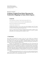
4.2.1. Finite System Power Index Samples. Figure 1 shows the
sensitivity of the weighted throughput achieved by the MAXFAIR algorithm as a function of the number of samples used
to obtain these values. The last point in the horizontal axis
corresponds to the optimal value. It should be noted that
in the vertical axis, the depicted weighted throughputs are
normalized over the optimal value. Moreover, the different

1
Normalised weighted throughput

10

0.95
0.9
0.85
0.8
0.75
0.7
10

20
50
100
200
Optimal
Number of system power index samples between (0,1)
5: [0, 1] dB
10: [0, 1] dB
20: [0, 1] dB
40: [0, 1] dB

5: [−3, 3] dB
10: [−3, 3] dB
20: [−3, 3] dB
40: [−3, 3] dB

Figure 1: The impact of number of samples on the weighted

throughput (MAX-FAIR).

curves provided in this figure correspond to different
combinations of the SNR ranges and the number of active
users. As can be seen, the more samples we choose, the
closer is the obtained maximum value to the optimal value,
which clearly presents the tradeoff between the accuracy
and the required computational power, as discussed before
in Section 3.3. For instance, we observe that in the cases
with small SNR range (e.g., [0,1] dB), even 20 samples are
sufficient to get satisfactory results, while for the cases with
larger SNR range (e.g., [−3,3] dB), more samples may be
required.
Furthermore, as it can be observed from this figure, for
the case of [0,1] dB, the larger the number of active users
in the system, the less sensitive is the achievable maximum
result to the number of samples (i.e., the slope of the
corresponding curve becomes smoother as the number of
active users increases). On the other hand, when there are
users with high SNR values (e.g., [−3,3] dB), the increasing
number of active users makes the achieved throughput drop
slightly for small number of samples. This difference in the
system behavior is closely related to a different number of
simultaneously served users, under different SNR ranges and
channel conditions, as depicted by the different observed
service patterns in Figure 2.
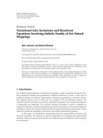
Specifically, in Figure 2, we present the probabilities of
the number of simultaneously served users in each scheduling cycle. For this experiment, we consider 40 backlogged
users in the system and perform 200 trials. In each trial,
users are randomly assigned the SNRs in the designated

SNR range, following the 8-state model [30] described in
Section 4.1. We observe that when there are users having
high SNR values, for example, in the cases of [−3,3] dB and
[2,4] dB, only a small number of users (at most 2 in this
experiment), are served concurrently. However, in the case


EURASIP Journal on Wireless Communications and Networking

11

Table 1: Channel state transition probability.

ps,s
ps,s−1
ps,s+1

s=1
0.9304
0
0.0696

s=2
0.8419
0.069
0.0891

s=3
0.8170
0.0879

0.0951

s=4
0.8216
0.0894
0.089

s=5
0.8349
0.0876
0.0775

3
−3
−4
0
2

4
0
−3
1
3

5
0
−3
1
3

6
0
−3
1
3

7
3
−2
1
4

that all users have small SNR values, for example, in the case
of [−4,−2] dB, the number of simultaneously served users
increases significantly (it is distributed between 4 and 17 in
our case as can be seen by Figure 2). Such user distribution
indicates that in the case that a single user cannot consume all
the system resources (e.g., the case where users have low SNR
values), more users will be scheduled simultaneously in order
to achieve a more efficient resource utilization and as a result
increase the total system throughput. This also demonstrates
the advantage of our proposed scheduling algorithm over the
one-by-one scheduling algorithms that have been proposed
in literature. As a result, with respect to Figure 1, for the
case of [0,1] dB, multiple users are scheduled to reach the
maximal throughput. Increasing the number of active users
enables the system to schedule more available candidates
to achieve higher throughput, and therefore the achievable
result is less sensitive to the number of samples. However, for
the case [−3,3] dB at most only 1 or 2 users are scheduled

for simultaneous transmission. In the following experiments
and numerical results, we adopt the accuracy of 100 samples,
which is sufficient to reach 95% of the optimal-weighted
throughput.
4.2.2. Parameter Convergence by Stochastic Approximation.
As described in Sections 2.1 and 3.4, parameters wi ’s are
used to represent the fairness constraints in our optimization
problem formulation. Figure 3 shows the dynamic change
of parameters wi ’s as the system and time evolve , for two
different cases that correspond to two different SNR ranges.
A seven-user scenario is considered, while for demonstration
purposes for each case the corresponding values of only
two representative users are presented—one user with strong
channel and one user with weak channel. As mentioned
before, all the users are assigned the same weight in order
to more clearly demonstrate the influence of the channel
conditions on wi ’s. It can be seen by this figure that the
converged values of wi ’s have the effect of compensating users
with the weak channels and reducing the priority of users
with strong channels in the scheduling policy. In fact, the
converged values of wi ’s will make both users (weak and
strong) to gain proper system resources and therefore achieve
fair throughput. Please note that it is the relative values of wi ’s

s=8
0.9616
0.0384
0

0.9

0.8
0.7
Probability

Case: [−3, 3]
Case: [−4, −2]
Case: [0, 1]
Case: [2, 4]

2
−3
−4
0
2

s=7
0.8945
0.0637
0.0418

1

Table 2: Simulation cases with different SNR(dB) distribution.
1
−3
−4
0
2

s=6

0.8590
0.0777
0.0633

0.6
0.5
0.4
0.3
0.2
0.1
0

0

2

4
6
8
10
12
14
Number of simultaneously served users

[−4, −2] dB
[0, 1] dB

16

18

[−3, 3] dB
[2, 4] dB

Figure 2: The service pattern under different channel conditions
(i.e., SNRs) (MAX-FAIR).

that control the priority of accessing the system resources,
and not their absolute values. Furthermore, it should be
noted that the lower the average SNR of a weak user, the
larger the gap between the weak user and a strong user, which
has negative impact on the achievable system throughput, as
we will see in the following subsection.
4.2.3. Throughput and Fairness Performance. Figure 4 shows
the average throughputs of all the users under the MAXFAIR, MAX, and HDR methods, for a seven-user scenario
where the average SNR range is [−3,3] dB and the corresponding average SNR assignments to the seven users
are as shown in Table 2. In order to better demonstrate
the tradeoff between the computational complexity and the
achievable throughput of MAX-FAIR approach, we obtained
the corresponding results under two different cases with
respect to the number of power index samples (i.e., 20
and 100 samples). As observed in this figure the MAXFAIR with 100 power index samples achieves slightly higher
throughput, however it requires five times the computational
power of the MAX-FAIR with 20 power index samples.
When compared to other two scheduling schemes, MAXFAIR presents the best throughput-fairness performance
(balances the achievable throughput of all users) despite
the variable channel conditions of the different users,
which indicates that the fairness is well maintained under
the proposed scheduling algorithm. As mentioned before
in the paper, the main objective of HDR is to achieve

12

EURASIP Journal on Wireless Communications and Networking
×104

9

7
8
−3 dB

6

6

Standard deviation

Control weight

7

0 dB
5
4
3

1 dB
3 dB

2
1

5
4
3
2
1

0

40

60

80

100

120

140

160

180

200

Time (s)
Case: [0, 1] dB
Case: [−3, 3] dB

Figure 3: The convergence of wi ’s for different users and different
SNR ranges (MAX-FAIR).

0
[−3, 3]

[−4, −2]
[0, 1]
SNR range (dB)

[2, 4]

MAX-FAIR
HDR
MAX

Figure 5: Standard deviation of achievable average throughputs.

×105

2

Average throughput (bits/s)

1.8
1.6

1.4
1.2
1
0.8
0.6
0.4
0.2
0

1

2

3

4
5
User ID

MAX-FAIR (20 samples)
MAX-FAIR (100 samples)

6

7

HDR
MAX

Figure 4: Average throughput for the [−3,3] dB case.

temporal fairness. Therefore, under HDR scheduling each
user throughput is closely related to its channel conditions.
That is why in Figure 4 we observe that users 1, 2, and 3 have
smaller throughput than users 4, 5, and 6, while user 7 has the
largest throughput under the HDR scheme. Under the MAX
algorithm, user 7 consumes most of the system resources
and achieves much higher throughput than the rest of the
users due to the fact that the objective of MAX algorithm
is to achieve the highest possible total system throughput,
without however considering the fairness issue. In Figure 5,
we further measure and evaluate the fairness performance by
the standard deviation of the average throughput under all

the four different SNR cases. Among the three algorithms,
MAX-FAIR algorithm has the smallest deviation for all the
different cases under consideration, while the corresponding
values change only slightly from case to case. We also find
that in general the standard deviation increases as the SNRs
become higher. This happens because small fluctuation of
wi results in larger throughput change, if all the users have
higher SNR levels.
Figure 6 compares the corresponding average system
throughputs of the three algorithms under evaluation, for
the different SNR ranges (cases). As we expected, MAX-FAIR
outperforms HDR in most cases due to the simultaneous
scheduling of multiple users, as has been demonstrated
in Figure 2, and consequently results in higher resource
utilization. However, in the case of SNR range of [−3,3] dB,
MAX-FAIR achieves slightly lower throughput than the

HDR. The reason of that resides in the different fairness
criteria considered and satisfied in these two algorithms,
namely, the throughput fairness and temporal fairness. If
we examine again Figure 3, we notice that users that have
low average SNR (−3 dB) (e.g., users 1, 2, and 3) finally
converge to a high wi , which enables them to have equal
opportunity to transmit under the MAX-FAIR scheduling
policy. Due to their weak channel conditions, their average throughputs will be low and hence the total system
throughput will become lower because of the satisfaction of
the throughput fairness constraint. However, as explained
before since access time is not the only resource to be
shared among the users in these systems, considering
throughput fairness instead of temporal fairness is more
meaningful in these systems and environments, despite
the slightly lower total throughput that can be achieved
in some cases under this consideration. One possible
alternative solution is to relax the fairness constraint if
the QoS permits it. Our experiments have demonstrated


EURASIP Journal on Wireless Communications and Networking

13

×105

450

6

Total throughput (KBits/s)

Total system throughput (bits/s)

400
5
4
3
2

350
300
250
200

1
150
0

[−3, 3]

[−4, −2]
[0, 1]
SNR range (dB)

0

5

10

[2, 4]

15
20
25
Number of users

30

35

40

MAX-FAIR
MAX

MAX-FAIR
HDR
MAX

Figure 8: System throughput as a function of the number of
backlogged users.

Figure 6: Achieved system throughput under different SNR ranges.

×104

5

15

4

13.33

3.5

11.66
10

3
2.5

8.33

2

wi

Average throughput (bits/s)

4.5

6.66
5

1.5
1

3.33

0.5

schedules the transmissions and distributes the resources
so that the various users achieve throughput according to
their corresponding assigned weights. Specifically users with
weights 2 and 4 obtain, respectively, two times and four
times the throughput achieved by users with weight 1. In this
figure, we also present (on the right-hand side vertical axis)
the converged values of parameters wi ’s. Here, the different
values of wi ’s reflect both the channel condition variations
and the weight differences. Please note that the relationship
between wi and weight is not linear due to the nonlinearity
between the allocated resources and throughput.

1.66

0

1

2

3

4
5
User ID

6

7

0

Throughput
wi

Figure 7: Average throughput under different QoS requirements
(weights) by MAX-FAIR.

that after relaxing fairness to 85% of its original requirement, the MAX-FAIR catches up and outperforms the
HDR.
In order to obtain a more in-depth understanding of
the MAX-FAIR fairness operation, in Figure 7, we present
the achieved average throughputs for all the seven users
under MAX-FAIR scheme, for a scenario where the SNR
range is assumed to be [−3,3] dB, and the users are
assigned different weights. The different weights can be
considered as the mapping of different QoS requirements.
In this scenario, users 1 and 4 have weight 1, users 2
and 5 have weight 2, while users 3, 6, and 7 have weight
4. Figure 7 demonstrates that the MAX-FAIR successfully

4.2.4. Number of Users. Figure 8 shows the achieved total
system throughput under MAX and MAX-FAIR algorithms
as a function of the number of backlogged users, for the
case where the users SNRs are located within [0,1] dB
range. Please note that as mentioned before MAX algorithm

provides the maximum uplink transmission throughput
without considering the fairness property, and therefore
is assumed to provide the upper bound throughput in
uplink scheduling. From this figure, we can clearly observe
the great advantage of the proposed MAX-FAIR approach
and its ability to achieve very high throughput, while still
maintaining fairness. When the number of backlogged users
reaches a certain level, for example, 35 in this experiment,
the throughput becomes flat for both MAX-FAIR and MAX,
which means that the chances of improving the throughput
by opportunistic scheduling with multiple users have been
fully utilized.

5. Conclusions
In this paper, the CDMA uplink throughput maximization
problem, while maintaining throughput fairness among the


14

EURASIP Journal on Wireless Communications and Networking

various users, was considered. It was shown that such a problem can be expressed as a weighted throughput maximization
problem, under certain power and QoS requirements, where
the weights are the control parameters that reflect the
fairness constraints. A stochastic approximation method
was presented in order to effectively identify the required
control parameters. The numerical results presented in
the paper, with respect to the convergence of the control
parameters and the achievable fairness, demonstrated that

this method is very effective in approximating the optimal
values and therefore controlling and maintaining fairness.
Furthermore, the concept of power index capacity was used
to represent all the corresponding constraints by the users
power index capacities at some certain system power index.
Based on this, the optimization problem under consideration
was converted into a binary knapsack problem, where the
optimal solution can be obtained through a global search
within a specific range.
The performance of the proposed policy in terms of
the achievable fairness and throughput was obtained via
modeling and simulation and was compared with the performances of other scheduling algorithms. The corresponding
results revealed the advantages of the proposed policy over
other existing scheduling schemes and demonstrated that
it achieves very high throughput, while satisfies the QoS
requirements and maintains fairness among the users, under
different channel conditions and requirements.

[9]

[10]

[11]

[12]

[13]

[14]

[15]

Acknowledgment
This work has been partially supported by EC EFIPSANS
Project (INFSO-ICT-215549).

References
[1] F. Adachi, M. Sawahashi, and H. Suda, “Wideband DS-CDMA
for next-generation mobile communications systems,” IEEE
Communications Magazine, vol. 36, no. 9, pp. 56–69, 1998.
[2] K. D. Wong and V. K. Varma, “Supporting real-time IP multimedia services in UMTS,” IEEE Communications Magazine,
vol. 41, no. 11, pp. 148–155, 2003.
[3] R. Berezdivin, R. Breinig, and R. Topp, “Next generation
wireless communications concepts and technologies,” IEEE
Communications Magazine, vol. 40, no. 3, pp. 108–116, 2002.
[4] N. R. Sollenberger, N. Seshadri, and R. Cox, “The evolution
of IS-136 TDMA for third-generation wireless services,” IEEE
Personal Communications, vol. 6, no. 3, pp. 8–18, 1999.
[5] J. Ramis, L. Carrasco, G. Femenias, and F. Riera-Palou,
“Scheduling algorithms for 4G wireless networks,” IFIP International Federation for Information Processing, vol. 245, pp.
264–276, 2007.
[6] P. Viswanath, D. N. C. Tse, and R. Laroia, “Opportunistic
beamforming using dumb antennas,” IEEE Transactions on
Information Theory, vol. 48, no. 6, pp. 1277–1294, 2002.
[7] P. Bender, P. Black, M. Grob, R. Padovani, N. Sindhushayana,
and A. Viterbi, “CDMA/HDR: a bandwidth-efficient highspeed wireless data service for nomadic users,” IEEE Communications Magazine, vol. 38, no. 7, pp. 70–77, 2000.
[8] F. Berggren, S.-L. Kim, R. Jă ntti, and J. Zander, “Joint power
a
control and intracell scheduling of DS-CDMA nonreal time

[16]

[17]

[18]

[19]

[20]

[21]

[22]

[23]

data,” IEEE Journal on Selected Areas in Communications, vol.
19, no. 10, pp. 1860–1870, 2001.
A. Jalali, R. Padovani, and R. Pankaj, “Data throughput
of CDMA-HDR a high efficiency-high data rate personal
communication wireless system,” in Proceedings of the 51st
IEEE Vehicular Technology Conference (VTC ’00), vol. 3, pp.
1854–1858, Tokyo, Japan, May 2000.
M. Andrews, K. Kumaran, K. Ramanan, A. Stolyar, P. Whiting,
and R. Vijayakumar, “CDMA data QoS scheduling on the
forward link with variable channel conditions,” Bell Labs
Technical Memorandum 10009626-000404-05TM, Bell Labs,
Paris, France, April 2000.
M. Andrews, K. Kumaran, K. Ramanan, A. Stolyar, P. Whiting,
and R. Vijayakumar, “Providing quality of service over a

shared wireless link,” IEEE Communications Magazine, vol. 39,
no. 2, pp. 150–154, 2001.
S. Shakkottai and A. Stolyar, “Scheduling for multiple flows
sharing a time-varying channel: the exponential rule,” Tech.
Rep., Bell Labs, Paris, France, 2000.
X. Liu, E. K. P. Chong, and N. B. Shroff, “Transmission
scheduling for efficient wireless utilization,” in Proceedings of
the 20th Annual Joint Conference of the IEEE Computer and
Communications Societies (INFOCOM ’01), vol. 2, pp. 776–
785, Anchorage, Alaska, USA, April 2001.
X. Liu, E. K. P. Chong, and N. B. Shroff, “A framework
for opportunistic scheduling in wireless networks,” Computer
Networks, vol. 41, no. 4, pp. 451–474, 2003.
Y. Liu and E. Knightly, “Opportunistic fair scheduling over
multiple wireless channels,” in Proceedings of the 22nd Annual
Joint Conference on the IEEE Computer and Communications
Societies (INFOCOM ’03), vol. 2, pp. 1106–1115, San Francisco, Calif, USA, March 2003.
S. A. Jafar and A. Goldsmith, “Adaptive multirate CDMA
for uplink throughput maximization,” IEEE Transactions on
Wireless Communications, vol. 2, no. 2, pp. 218–228, 2003.
L. Xu, X. Shen, and J. W. Mark, “Dynamic bandwidth
allocation with fair scheduling for WCDMA systems,” IEEE
Wireless Communications, vol. 9, no. 2, pp. 26–32, 2002.
C. Li and S. Papavassiliou, “Fair channel-adaptive rate
scheduling in wireless networks with multirate multimedia
services,” IEEE Journal on Selected Areas in Communications,
vol. 21, no. 10, pp. 1604–1614, 2003.
J. Cho and D. Hong, “Tradeoff analysis of throughput and
fairness on CDMA packet downlinks with location-dependent
QoS,” IEEE Transactions on Vehicular Technology, vol. 54, no.

1, pp. 259–271, 2005.
S. S. Kulkarni and C. Rosenberg, “Opportunistic scheduling
policies for wireless systems with short term fairness constraints,” in Proceedings of IEEE Global Telecommunications
Conference (GLOBECOM ’03), vol. 1, pp. 533–537, San
Francisco, Calif, USA, December 2003.
C. Li and S. Papavassiliou, “Opportunistic scheduling with
short term fairness in wireless communication systems,” in
Proceedings of the Conference on Information Sciences and
Systems (CISS ’04), pp. 167–172, Princeton, NJ, USA, March
2004.
S. Ramakrishna and J. M. Holtzman, “A scheme for throughput maximization in a dual-class CDMA system,” IEEE Journal
on Selected Areas in Communications, vol. 16, no. 6, pp. 830–
844, 1998.
T. Ottosson and A. Svensson, “On schemes for multirate
support in DS-CDMA systems,” Wireless Personal Communications, vol. 6, no. 3, pp. 265–287, 1998.


EURASIP Journal on Wireless Communications and Networking
[24] S. Borst and P. Whiting, “Dynamic rate control algorithms
for HDR throughput optimization,” in Proceedings of the
20th Annual Joint Conference of the IEEE Computer and
Communications Societies (INFOCOM ’01), vol. 2, pp. 976–
985, Anchorage, Alaska, USA, April 2001.
[25] A. Sampath, P. S. Kumar, and J. M. Holtzman, “Power control
and resource management for a multimedia CDMA wireless
system,” in Proceedings of the 6th IEEE International Symposium on Personal, Indoor and Mobile Radio Communications
(PIMRC ’95), vol. 1, pp. 21–25, Toronto, Canada, September
1995.
[26] C. Li and S. Papavassiliou, “Joint throughput maximization
and fair scheduling in uplink DS-CDMA systems,” in Proceedings of IEEE/Sarnoff Symposium on Advances in Wired and

Wireless Communication, pp. 193–196, Princeton, NJ, USA,
April 2004.
[27] D. S. Hochbaum, “A nonlinear Knapsack problem,” Operations
Research Letters, vol. 17, no. 3, pp. 103–110, 1995.
[28] S. Martello and P. Toth, Knapsack Problems: Algorithms and
Computer Implementations, John Wiley & Sons, New York, NY,
USA, 1990.
[29] R. Miller, Optimization: Foundations and Applications., John
Wiley & Sons, New York, NY, USA, 2000.
[30] H. Wang and N. Moayeri, “Finite-state Markov channel—
a useful model for radio communication channels,” IEEE
Transactions on Vehicular Technology, vol. 44, no. 1, pp. 163–
171, 1995.

15