Báo cáo hóa học: "Research Article Spatial and Temporal Fairness in Heterogeneous HSDPA-Enabled UMTS Networks" docx

Hindawi Publishing Corporation
EURASIP Journal on Wireless Communications and Networking
Volume 2009, Article ID 682368, 12 pages
doi:10.1155/2009/682368
Research Article
Spatial and Temporal Fair ness in Heterogeneous HSDPA-Enabled
UMTS Networks
Andreas M
¨
ader
1
and Dirk Staehle
2
1
Department of Distributed Systems, University of Wuerzburg, Sanderring 2, 97070 W
¨
urzburg, Germany
2
NEC Laboratories Europe, Kurfuersten-Anlage 36, 69115 Heidelberg, Germany
Correspondence should be addressed to Andreas M
¨
ader,
Received 15 July 2008; Revised 27 November 2008; Accepted 29 December 2008
Recommended by Ekram Hossain
The system performance of an integrated UMTS network with both High-Speed Downlink Packet Access users and Release ’99 QoS
users depends on many factors like user location, number of users, interference, multipath propagation profile, and radio resource
sharing schemes. Additionally, the user behavior is an important factor; users of Internet best-effort applications tend to follow a
volume-based behavior, meaning they stay in the system until the requested data is completely transmitted. In conjunction with
the opportunistic transmission scheme implemented in HSDPA, this has implications to the spatial distribution of active users as
well as to the time-average user and cell throughput. We investigate the relation between throughput, volume-based user behavior
and traffic dynamics with a simulation framework which allows the efficient modeling of large UMTS networks with both HSDPA

and Release ’99 users. The framework comprises an HSDPA MAC/physical layer abstraction model and takes network aspects like
radio resource sharing and other-cell interference into account.
Copyright © 2009 A. M
¨
ader and D. Staehle. This is an open access article distributed under the Creative Commons Attribution
License, which permits unrestricted use, distribution, and reproduction in any medium, provided the original work is properly
cited.
1. Introduction
Mobile network operators continue to deploy the High-
Speed Downlink Packet Access (HSDPA) service in their
existing Universal Mobile Telecommunication System
(UMTS) networks. From the users perspective, the HSDPA
promises high data rates (up to 14.4 Mbps with Release
5) and low latency. From the perspective of an operator,
HSDPA is hoped to play a key role for the much longed for
breakthrough of high-quality mobile data services. From a
technical perspective, HSDPA introduces a new paradigm
to UMTS; instead of adapting the transmit power to the
radio channel condition in order to ensure constant link
quality, HSDPA adapts the link quality to the radio channel
conditions. This enables a more efficient use of scarce
resources like transmit power, channelization codes, and also
hardware components.
The basic principle of the HSDPA is to adapt the
link to the instantaneous radio channel condition using
adaptive modulation and coding (AMC). HSDPA employs a
shared channel, the High-Speed Downlink Shared channel
(HS-DSCH), which is used by all HSDPA users. With a
shared channel, radio resources are occupied only if a
transmission occurs, which enables a more efficient transport

of bursty traffic. In each transport time interval (TTI), the
scheduler located in the NodeB decides about the users
to be scheduled and about their data rate. The scheduling
decision can be either on behalf of channel quality indicator
(CQI) reports from the user equipments (UE) to enable
opportunistic scheduling schemes which use the air interface
more efficiently, or simple nonopportunistic schemes like
round-robin can be used which shares the resources time fair
among the users.
An important aspect of HSDPA systems is the perceived
fairness of the connection metrics between the users. This
is in contrast to pure UMTS Release ’99, where the circuit-
switched design of the radio bearers guarantees equal
QualityofService(QoS)propertiesofallusersofthesame
service class [1]. However, since in HSDPA the theoretically
achievable data rate depends on the channel condition,
the actual achieved data rates depend on user location,
number of users, interference, scheduling discipline, and in
2 EURASIP Journal on Wireless Communications and Networking
integrated networks also on the number of dedicated channel
(DCH) connections. In this work, we distinguish between
two fairness aspects. Spatial fairness refers to the spatial
distribution of the perceived data rates within a cell or sector.
Temporal fairness refers to the long-term time-average user
throughput [2].
Our contribution is twofold: first, we propose a flow-
level simulation framework which takes on the one hand
physical layer aspects, scheduling disciplines, interference,
and radio resource management schemes into account, but
also allows for simulation of large networks due to its

analytical approach. Second, we investigate the impact of
three well-known scheduling disciplines, namely round-
robin, proportional fair, and Max C/I on the spatial user
distribution and on the system and user performance. One
of our main findings is that Max C/I scheduling, although
providing sum-rate optimal rate allocations in static system
scenarios, performs worse than proportional fair scheduling
if traffic dynamics are considered.
The remaining of this article is organized as follows:
in the next section, we motivate our work and give an
overview of the current literature. In Section 3,wegivea
brief overview of the HSDPA. In Section 4, we explain radio
resource sharing between DCH and HSDPA connections and
formulate a model for the calculation of NodeB transmit
powers. In Section 6, a physical layer abstraction model for
the HSDPA is proposed which enables the calculation of
the average throughputs per flow for different scheduling
disciplines. Simulation scenarios and numerical results are
presented in Section 7, followed by a conclusion in Section 8.
2. Motivation and Related Work
The focus of this work is the impact of elastic flows on the
system performance. We have to distinguish between QoS
flows which require a fixed bandwidth, as for voice calls over
DCH transport channels, and “best-effort” or elastic flows
which adapt their bandwidth requirements to the currently
available bandwidth. Such a flow may be an FTP transfer or
the combined elements of a web page including inline objects
such as embedded videos, that may be transmitted in parallel
TCP connections. A flow can be loosely defined as a coherent
stream of data packets with the same destination address [3].

An important distinction between the two types of flows is
that QoS flows typically follow a time-based trafficmodel,
which means that the user wants to keep the connection for a
certain time span. In contrast, elastic flows are volume-based,
that is, the user is satisfied as soon as a certain data volume is
transmitted. An effect in this context which is that of spatial
inhomogeneity, which has been mentioned in [4] for systems
without AMC, and has been further investigated in [5, 6]
for pure single-cell HSDPA systems. Users with bad radio
conditions experience lower data rates than users with better
radio conditions, leading to a spatial unfairness, which we
define as the discrepancy between location-dependent user
arrival probabilities and the observed residence probabilities
in steady state. We investigate this effect in Section 7.1 for
different scheduling disciplines in a multicell scenario, that
is, with consideration of other-cell interference, and with
location-dependent arrival rates.
A related point is the system performance and fairness
of the perceived data rates under different scheduling
regimes. In the literature, a large number of fundamental
works investigate the tradeoff between fairness and system
capacity in a wireless systems with opportunistic scheduling.
Examples can be found in [2, 7–10], where in [7] the
concept of multiuser diversity (MUD) in downlink direction
has been investigated, motivated by the findings in [11]
for the uplink direction. For HSDPA systems, research
mainly concentrated on variations of the proportional fair
scheduler developed for the 1xEV-DO system [12]. Different
approaches exist to include QoS constraints on delay or
data rate into the scheduling decision [13–17]. The fairness

of different schedulers in HSDPA systems is investigated in
[18, 19]. Both works conclude that Max C/I provides the
highest system throughput. We compare user and system
throughput for round-robin, Max C/I, and proportional
fair scheduling. The results show that on the one hand, as
expected the two channel-aware schemes clearly outperform
round-robin scheduling, but on the other hand, proportional
fair scheduling leads to a higher time-average throughput
than Max C/I scheduling. We discuss this result in detail in
Section 7.2.
Statistically valid results for integrated UMTS networks
require long simulation runs or analytical approaches. An
intuitive example is the DCH blocking probability; a DCH
user which is located far from the antenna is subject to strong
interference from surrounding NodeBs, he may therefore
require a very high transmit power. If this user additionally
has a long call time, the influence on the blocking probability
is significant. Since such events occur not very often with
reasonable loads, long simulation runs are required. The
results in this work are therefore generated with a simulation
framework based on [20, 21], that uses analytic methods
to approximate the effects of the physical layer and the
scheduling discipline on flow level. This allows for accurate
and time-efficient simulations of large UMTS networks.
3. System Description
We consider a UMTS network where HSDPA and DCH
connections share the same radio resources, namely transmit
power and channelization codes. The core of the HSDPA is
the HS-DSCH, which uses up to 15 codes with spreading
factor (SF) 16 in parallel. The HS-DSCH enables two types

of multiplexing; time multiplex by scheduling the subframes
to different users, and code multiplex by assigning each user
a nonoverlapping subset of the available codes. The latter
requires the configuration of additional High-Speed Shared
Control Channels (HS-SCCHs). Throughout this work we
assume that only one HS-SCCH is present, hence consider
time multiplex only.
In contrast to dedicated channels, where the transmit
power is adapted to the propagation loss with fast power
control and thus enabling a more or less constant bit rate,
the HS-DSCH adapts the channel to the propagation loss
EURASIP Journal on Wireless Communications and Networking 3
Scheduling
decisions
CQI reporting
2ms
TTI
SF 16 codes
UE 1
UE 2
UE 3
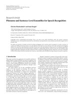
Figure 1: Schematic view of the HSDPA transport channel.
with AMC. The UE sends CQI values to the NodeB. The
CQI is a discretization of the received signal-to-interference
ratio (SIR) at the UE and ranges from 0 (no transmission
possible) to 30 (best quality). The scheduler in the NodeB
then chooses a transport format combination (TFC) such
thatapredefinedtargetBLER,whichisoftenchosenas10%,
is fullfilled if possible. The TFC contains information about
the modulation (QPSK or 16QAM), the number of used

codes (from 1 to 15), and the coding rate resulting in a certain
transport block size (TBS) that defines the information bits
transmitted during a TTI. A number of tables in [22]define
a unique mapping between CQI and TFC. This means that
with an increasing CQI, the demand on code resources is also
increasing. This leads to cases where a high CQI is reported
to the NodeB, but the scheduler has to select a lower TBS due
to lacking code resources. A schematic view of the HSDPA
functionality is shown in Figure 1.
4. Sharing Code and Power Resources between
HSDPA and DCH
A key issue of the radio resource management in HSDPA
enhanced UMTS networks is the sharing of code and power
resources between DCHs, signaling channels, common chan-
nels, and finally channels required for the HSDPA, namely,
the HS-DSCH and the HS-SCCH. The signaling channels
and common channels mostly require a fixed channelization
code and a fixed power as for the pilot channel (CPICH)
or the forward access channel (FACH). The DCHs are
subject to fast power control which means that their power
consumption depends on the cell or system load that
determines the interference at the UE. The general level of
power consumption depends on the processing gain and the
required target bit-energy-to-noise ratio (E
b
/N
0
) of the radio
access bearer (RAB).
The HSDPA requires code and power resources. Codes

are the channelization codes that are generated according to
the orthogonal variable spreading factor (OVSF) code tree.
The number of codes that is available for a certain spreading
factor (SF) is equal to the spreading factor itself. A 384 kbps
DCH occupies an SF 8 channelization code. Accordingly,
the maximum number of parallel 384 kbps users per sector
is theoretically 8. In practice, only 7 parallel 384 kbps users
are possible since the signaling and common channels also
require some code resources. Let us introduce an SF 512 code
as the basic code unit. Then, a DCH i with SF k occupies
c
i
= 512/k code resources. An HSDPA code with SF 16
requires c
HS
= 32 code resources. Let C
DCH
be the total
code resources occupied by all DCHs, C
CCH
be the resources
occupied by signaling and common channels, and, C
HS
=
n
HS
· c
HS
be the total number of code resources used by the
HSDPA where n

HS
is the number of SF 16 codes allocated
to the HS-DSCH. The total number of code resources is
equal to C
tot
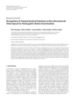
= 512. We consider adaptive code allocation
[23, 24], which is illustrated in a simplified view (pilot and
control channels are omitted) in Figure 2 for both transmit
power and channelization codes. We further assume that the
codes are always optimally arranged in the code tree, and
that no code tree fragmentation occurs. The number of codes
available for the HSDPA is then
n
HS
=

C
tot
−C
CCH
−C
DCH
c
HS

. (1)
Accordingly, the transmit power T
x,tot
consists of a
constant part T

CCH
for common and signaling channels, a
part T
DCH
for DCHs, and a part T
HS
for the HS-DSCH. Let
T
∗
be the target transmit power at the NodeB. Then, the HS-
DSCH power with adaptive power allocation is
T
HS
= T
∗
−T
CCH
−T
DCH
,(2)
where T
∗
HS
is the power reserved for the HS-DSCH, and T
DCH
is the total DCH power averaged over some period of time.
5. Calculation of Downlink Transmit Powers
We define a UMTS network as a set L of NodeBs with
associated UEs, M
x

. A DCH connection k corresponds to a
radio bearer at NodeB x
∈ L with data rate R
k
and code
resource requirements c
k
. Since the power consumed by the
DCH connection is subject to power control, the received
E
b
/N
0
ε
k
fluctuates around a target-E
b
/N
0
value ε
∗
k
,which
is adjusted by the outer-loop power control such that the
negotiated QoS parameters like frame error rate are fulfilled.
A common approximation for the average E
b
/N
0
value is

ε
k
=
W
R
k
·
T
k,x
·d
k,x
W ·N
0
+ I
k,oc
+ α
i
·T
x,tot
·d
k,x
,(3)
where the orthogonality α
k
describes the impact of the
multipath profile for DCH k, d
k,x
is the average path gain
between NodeB x and UE k, W is the system chip rate, and
N

0
is the thermal noise density. We assume perfect power
control, that is, the mean E
b
/N
0
value meets exactly the
target-E
b
/N
0
such that ε
k
= ε
∗
k
. The mean transmit power
requirement of a DCH connection follows then as
T
k,x
=
ε
∗
k
·R
k
W
·

W ·N

0
+ I
k,oc
d
k,x
+ α
k
·T
x,tot

. (4)
4 EURASIP Journal on Wireless Communications and Networking
Time Time
Tr an sm i t po we r
Channelization codes
T
HSDPA
T
non-HSDPA
T
max
C
max
C
HSDPA
C
non-HSDPA
Adaptive radio resource allocation
Figure 2: Adaptive radio resource management scheme.
The average other-cell interference comprises the

received powers of surrounding NodeBs such that
I
k,oc
=

y∈L\x
T
y,tot
· d
k,y
. The total NodeB transmit
powers can be calculated with an equation system over all
NodeBs. For that reason, we follow [25] and define the load
of NodeB x with respect to NodeB y as
η
x,y
=

k∈M
x
ω
k,y
,
with ω
k,y
=
ε
∗
k
·R

k
W
·
⎧
⎪
⎨
⎪
⎩
α,ifL(k) = y,
d
k,y
d
L(k)
, k
,ifL(k)
/
= y.
(5)
After some algebraic modifications, this allows us to formu-
late the total DCH transmit power in a compact form as
T
x,DCH
=

y∈L
η
x,y
·T
y,tot
. (6)

In this equation, we neglect the thermal noise since in a
reasonable designed network its impact on the transmit
power requirements is minimal. Note also that the equation
includes the case y
= x for the own-cell interference. For the
total transmit power we introduce the boolean variable δ
y,HS
indicating whether at least one HSDPA flow is active in cell
x. The total transmit power at NodeB x is then
T
x,tot
= δ
x,HS
·T
∗
x
+

1 − δ
x,HS

·

T
x,CCH
+

y∈L
η
x,y

·T
y,tot

.
(7)
This equation states that if the HS-DSCH is active, the total
transmit power is equal to the target power. Otherwise, it
consist only of the DCH transmit power and the transmit
power for common channels. Introducing the vectors
V[x]
= δ
x,HS
·T
∗
x
+

1 − δ
x,HS

·T
x,CCH
,(8)
and matrix
M[x, y]
=

1 − δ
x,HS


·
η
x,y
(9)
leads to the matrix equation
T
= V + M ·T ⇐⇒ T = (I − M)
−1
·V, (10)
which provides the transmit powers of all NodeBs in the
system. The matrix I is the identity matrix, and T is the
vector of NodeB transmit powers T
x
. The DCH and HSDPA
transmit powers are then calculated with (6)and(2).
6. HSDPA Physical Layer Model
Consider an HS-DSCH with power T
HS
= Δ
HS
·T
tot
and n
HS
parallel codes allocated to the HS-DSCH. Accordingly, the
SIR at UE i for a RAKE receiver with perfect maximum ratio
combining is equal to
γ
i
= Δ

HS
·

p∈P
T
tot
·d
i,p,x
W ·N
0
+ I
oc,i
+

r∈P \p
T
x,tot
·d
i,r,x
,
(11)
where d
i,p,x
is the instantaneous propagation gain of signal
path p
∈ P . The UE measures the SIR and maps it to the
maximum CQI with a transmission format that achieves a
frame error rate of 10%. In [26] the following relation of SIR
and CQI q is given:
q

= max

0, min

30,

SIR[dB]
1.02
+16.62

. (12)
The CQI-value q defines the maximum possible TBS
v(q), that can be transmitted in one TTI. It also defines the
number of required parallel codes n
HS
(q). If the number of
available codes n
HS
is less than n
HS
(q), the scheduler selects
the maximum possible TBS value according to n
HS
. This
means that an optimal usage of resources is only possible
if the transmission format according to the reported CQI
utilizes all available codes. If too few code resources are
available, power resources are wasted, and if too few power
resources are available, the CQI is too small to utilize all
available codes. The reported CQI value depends essentially

on the multipath profile, the users’ location, the available
HS-DSCH power, and the other-cell power. The number of
codes required for a certain CQI value depends on the CQI
category.
Above equations give the CQI and TBS for a concrete
instance of the propagation gains in particular of the
multipath component power. For a simplified simulation
and evaluation of the HSDPA performance, an approximate
model for the HSDPA bandwidth similar to the orthogo-
nality factor model for DCH is required. The orthogonality
factor [27] is used to determine the signal-to-interference
ratio for a DCH i as
γ
i
=
W
R
i
·
T
x
·d
x,i
I
i,other
+ α · I
i,own
, (13)
where W/R
k

is the processing gain, I
i,other
is the other-
cell interference, and I
i,own
= T
x,tot
· d
x,i
is the own-cell
EURASIP Journal on Wireless Communications and Networking 5
interference. The orthogonality factor α specifies the part of
the power received from the own cell that contributes to the
interference due to multipath propagation. It captures the
impact of the multipath profile in a single value between 0.05
and 0.4 depending on the multipath profile. For a deeper
discussion of the orthogonality factor model please refer to
[28–30] and the references therein.
Actually, the values γ
k
, I
own
,andI
other
are mean values
averaged over the short-term fading. More precisely, we
should write (13)as
E[γ
i
] =

W
R
i
·
T
x,i
·d
x,i
E

I
i,other

+ α · E

I
i,own

=
W
R
i
·
T
x,i
T
x,tot
·
1
E


I
i,other

/E

I
i,own

+ α
.
(14)
The orthogonality factor model is not applicable to the
HSDPA since it only yields the mean SIR. However, for the
evaluation of the average HSDPA data rate of a UE at a
certain location, the distribution of the reported CQI values
is required. The essential assumption of the orthogonality
factor model is that the mean normalized SIR, that is, the last
fraction in (14), is a function of the ratio Σ of average other-
cell received power and average own-cell received power (or
short other-to-own-cell power ratio)
Σ
i
=
E

I
i,other

E


I
i,own

=

y
/
=x
T
y,tot
·d
y,i
T
x,tot
·d
x,i
. (15)
In [20], the orthogonality factor model is enhanced to
yield not only the mean but also the standard deviation of
the SIR in decibel scale as a function of Σ
i
. Assuming that
the distribution of the SIR follows a normal distribution that
is entirely characterized by its mean and standard deviation,
the distribution of the reported CQI values, p
CQI
(q), is
obtained from the cumulative density function (CDF) of
the distribution of the SIR. Truncating the CQI distribution

according to the available codes for the HS-DSCH yields the
distribution of the TBS as
p
TBS
(v) =
⎧
⎪
⎪
⎨
⎪
⎪
⎩
p
CQI
(v(q)), if v(q) <v
∗
,
30

q=v
∗
p
CQI
(q), else,
(16)
where v
∗
is the maximum allowed TBS according to the
available code resources. Accordingly, we denote the CDF of
the CQI and TBS values with P

CQI
(q)andP
TBS
(v).
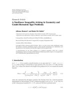
The physical layer abstraction model gives also insights
into the impact of system parameters like multipath channel
profile, number of available codes and, UE category. Figure 3
shows the gross data rate, that is, the throughput a single UE
would achieve, depending on the other-to-own-interference
ratio for the ITU Vehicular A, Pedestrian A, and Vehicular
B multipath propagation models. A profile with a strong
dominating path, like in Pedestrian A, enables indeed very
high data rates up to 13 Mbps. In contrast, profiles with a
relatively strong second path, like Vehicular A and Vehicular
B, lead to significantly lower data rates due to a higher
14
12
10
8
6
4
2
0
Mean TBS (kbit)
−30 −20 −10 0
Other-to-own cell power ratio Σ (dB)
ITU Pedestrian A
ITU Vehicular A
ITU Pedestrian B
Figure 3: Gross data rate for different channel profiles.

14
12
10
8
6
4
2
0
Mean TBS (kbit)
−30 −20 −10 0
Other-to-own cell power ratio Σ (dB)
UE cat. 10, Ped. A
UE cat. 9, Ped. A
UE cat. 7-8, Ped. A
UE cat. 1–6, Ped. A
UE cat. 1–10, Ped. B
UE cat. 11-12, Ped. B
UE cat. 11-12, Ped. A
Figure 4: Gross data rates for different UE categories.
intersymbol interference. In fact, with these two models,
it is sufficient to provide five SF 16 codes for the HS-
DSCH. Figure 4 shows the gross data rates for different UE
categories, which reflect the capability for 16QAM, number
of parallel codes and, interscheduling time. Interesting is
that UEs without QAM 16 support (categories 11 and 12)
have significantly lower data rates than UEs with QAM 16,
although the transport block sizes are identically (categories
1–6).
6.1. Scheduling. The scheduler in the NodeB has a large
influence on the user-level and system-level performance of

6 EURASIP Journal on Wireless Communications and Networking
the HSDPA. Several proposals exist for HSDPA scheduling,
from which we considered three of the most common
schemes. The channel-blind round-robin scheme selects
users consecutively for transmission. The MaxTBS-scheduler
chooses always the user with the currently best possible
TBS, including restrictions due to code resources. Finally,
the proportional fair scheduler selects the user which
has the proportionally best TBS in relation to its past
throughput.
Channel-aware schedulers like MaxTBS and propor-
tional fair benefit from multiuser diversity [7]. With an
increasing number of users in a cell, the probability to
see at least one user with good radio conditions also
increases. If “strong” users are favored by the scheduler,
the aggregated cell throughput increases. Exploitation of
multiuser diversity is therefore in the end beneficial for the
overall system capacity, also because reduced transmission
times for volume-based users leads to longer time periods
where the HS-DSCH is switched off—which in turn reduces
interference.
6.1.1. Round-Robin Scheduling. The round-robin scheduler
selects the users consecutively for transmission. In a suf-
ficiently long time interval, the probability that a user k
is selected is therefore approximately 1/
|M|. Round-robin
is a channel-blind scheduling discipline, which means that
the average throughput of each mobile depends only on
its channel condition and the number of users in the
cell, but not on the channel conditions of other users.

Consequently, the cell throughput does not benefit from
multiuser diversity. However, round-robin is robust and does
not suffer from any convergence issues like proportional fair
scheduling in some cases [31], and it is easy to implement
due to its simple principle. Round-robin is an allocation-
fair scheduling discipline in the sense that, to every user, the
same amount of radio resources in terms of codes and power
are allocated. This approach is often sufficient to prevent
starvation of users at the cell edge.
6.1.2. MaxTBS Scheduling. With MaxTBS (or Max C/I)
scheduling, the user with the currently best TBS is scheduled.
This scheduling discipline maximizes the sum-rate capacity
(in our context the cell throughput) given the saturated case,
that is, all users have at least one packet to transmit [32, 33].
If two or more users have the maximum possible TBS, a
random user out of this set is selected with equal probability.
In contrast to round-robin scheduling, the throughput of
a user depends not only on its own location, but also
on the location of the other users. In [6], this scheduling
discipline is modeled as a priority queue, where locations
closer to the NodeB have higher priority than locations
farther away. However, it is also possible to calculate the
average throughput directly from the TBS distributions of
the users. In this work we use the formulation we developed
in [21]. MaxTBS strongly favors the user with the best
channel quality. This implicates that users with weak radio
conditions are penalized and perceive on average very low
data rates, leading to unfair rate allocations. We show in the
next section how this behavior negatively affects the average
throughput if traffic dynamics are considered.

6.1.3. Proportional Fair Scheduling. Proportional fair (PF)
scheduling is a scheduling discipline which has been devel-
oped for the 1xEv-DO-system in the downlink [12]. The
basic principle is to allocate each user proportional to its link
quality and its past throughput. This is achieved by selecting
the user that has the best instantaneous relative throughput
over its past throughput, which is often calculated with
a sliding window approach. However, different versions of
PF scheduling exist. The most fundamental difference is
the way how the past throughput is calculated. The first
variant updates the past throughput every scheduling period
regardless whether the user has been scheduled or not, the
second variant updates the past throughput only if the user is
indeed chosen for transmission. The difference between both
versions is that in the first case the mean throughput of a user
is proportional to its channel quality only, while in the second
case it is also related to the generated traffic. In [31, 34]
it is argued that both variants approximately lead to the
same results in case of statistically identical fades and infinite
backlogs. The second assumption is reasonable during the
interevent time, while the first assumption is contradicted by
the fact that the shape of the CQI distribution depends on the
level of received other-cell interference. A direct formulation
of the flow-average throughput and a comparison between
both variants can be found in [21].
7. Flow-Level Performance Results
UMTS networks are dynamic systems because of the mutual
dependency among the transmit powers of different cells.
This means that a well-designed performance evaluation
has to consider networks with a reasonable size in order

to capture these effects and their impact on flow-level
performance properly. We consider two different types of
networks: a 19-NodeB hexagonal layout with a NodeB
distance of 1.2 km, and an irregular layout with 22 NodeBs
which is generated from a Voronoi tessellation. The network
areas are partitioned into area elements with an edge length
of 25 m. Figure 5 shows the irregular network with antenna
locations (dots) and arrival cluster centers (stars). In the
hexagonal layout, user arrive according to a homogeneous
Poisson process such that arrival rates are equal for all area
elements. In the irregular network, users arrive according to
a clustered Poisson process as described in [25] and shown in
Figure 6; the total arrival rate λ
f
in an area element f results
from the superposition of circular clusters with constant
arrival rates. In the irregular network therefore not only the
layout but also the arrival process is heterogeneous.
Results are generated with a time-dynamic simulation
which considers the HSDPA data trafficofauserasaflow
with a certain data volume. The network area is discretized
into a set of area elements with an edge length of 25 m.
The time axis is divided in interevent times. We assume that
between two events the users stay roughly within an area
element.
EURASIP Journal on Wireless Communications and Networking 7
1
2
3
4

5
6
7
8
9
10
11
12
13
14
15
16
17
18
19
20
21
22
7
6
5
4
3
2
1
(km)
1234567
(km)
Figure 5: Irregular network layout. Dots indicate NodeB (antenna)
locations, stars mark cluster centers.

7
6
5
4
3
2
1
(km)
1234567
(km)
Figure 6: Inhomogeneous arrival densities. Darker colors indicate
higher probability of arrival.
We consider two types of events: arrival events, that is,
the arrival of a new user into the system, and departure
events, which may occur if an HSDPA user has received
all its data or if the call time of DCH user is reached.
On arrival of a new user, admission control for DCH and
HSDPA is performed. The admission control for DCH
connections is threshold-based. An incoming connection
is blocked if the total transmit power including the new
connection exceeds the target transmit power, or if the
available code resources are not sufficient. For this purpose,
the required transmit power is calculated at the serving
NodeB under the worst-case assumption that all NodeBs
transmit with the target power in order to prevent possible
outage. For the HSDPA, we assume a count-based admission
control which restricts the maximum number of concurrent
connections to a fixed value. If the incoming connection is
admitted into the system, the call time or the data volume,
depending on the user type, is calculated according to the

respective distribution parameters. We assume exponentially
distributed call times with mean E[T]
= 120 s for DCH users
and exponentially distributed flow sizes with mean volume
E[V]
= 100 KB for HSDPA users. The arrival rate of the
DCH users is determined from the offered DCH code load
defined as
ρ
c
=

s∈S
λ
s
μ
s
·
c
s
C
tot
, (17)
where μ
s
= 1/E[T
s
], and the index s denotes the service class
of the radio bearer.
On each event, the system variables are recalculated

if necessary. If the event is generated by a DCH arrival
or departure, HSDPA code resources in the relevant cells
are decreased or increased according to the DCH code
requirements. Additionally, the total transmit powers are
updated for all NodeBs in order to capture the new inter-
ference situation. Transmit power recalculation is also done
if the HS-DSCH is switched on or off because of HSDPA
user arrivals or departures. In all cases, the data volume
transmitted by HSDPA users within the past interevent
time is subtracted from their remaining data volumes. New
HSDPA data rates are calculated, taking the new radio
resource and interference situation into account. Finally, the
expected departure times of the HSDPA users are updated
according to the remaining data volumes and data rates.
7.1. Volume-Based Traffic Model and Spatial Fairness. As
mentioned before, an important distinction between QoS
and elastic flows is that QoS flows typically follow a time-
based traffic model, which means that the user wants to
keep the connection a certain time span, for example, for the
time of a conversation. In contrast, elastic flows are volume-
based, that is, the user leaves the system as soon as a certain
data volume is transmitted. In reality, the user behavior is
a mixture between both models, depending on factors like
user satisfaction, pricing models, type of content. However,
the two models can be seen as the extremes of the actual user
behavior.
Atime-basedtraffic model implicates that the number of
currently active users is independent of the perceived data
rates. Moreover, the spatial distribut ion of the number of
users is corresponding to the spatial arrival process;ifusers

arrive with arrival rate λ, the number of concurrently active
users in steady-state follows according to Little as λ/μ,ifno
blocking occurs.
Avolume-basedtraffic model means that users stay
in the system until their service demands are fullfilled.
Therefore, the number of active users depends on the
assigned data rates. In HSDPA systems, the data rate depends
8 EURASIP Journal on Wireless Communications and Networking
on the channel quality, which means that users with low
average channel qualities stay longer in the system than
those with good channel qualities. Since the average channel
quality is dominated by the other-cell interference, users
at the cell edges stay longer in the system than users in
the center of the cell. This implies that the spatial arrival
process and the spatial steady state distribution are not
directly related anymore, a fact that complicates planning
of HSPDA networks significantly. One reason is that Monte
Carlo methods [35] now have to estimate the spatial user
population for every snapshot, which is difficult without
knowledge of the the currently ongoing flows. With round-
robin scheduling, a direct formulation of the mean transfer
time was found in [5, 24], since in that case the data rates
of the users only depend on the number of users and their
position, but are otherwise independent of each other.
We now clarify the effect of spatial heterogeneity with
some example scenarios. Figure 7 shows the arrival proba-
bility and the residency probability versus the distance to
the antenna for cell number 2 from the irregular scenario.
The arrival probability describes the probability that a user
arrives in this cell at a certain point, while the residence

probability reflects the spatial distribution of the users in the
cell in steady state. The spiky shape of the curves is due to the
discretization of the cell area into area elements. It is obvious
that arrival and residence probabilities are not equal, and that
the magnitude of the deviation depends on the scheduling
discipline. MaxTBS scheduling shows the highest deviation,
since users close to the antenna leave the system much earlier
than users farther away. An interesting result is that residence
probabilities with proportional fair scheduling fir slightly
better to the arrival probabilities if compared to round-robin
scheduling. We will see later that this effect comes from the
fact that the proportional fair scheduler favors users on the
cell edges.
Figure 8 shows the corresponding ratio between arrival
and residence probability in the same cell. With time-based
users, the ratio would be equal to one at all distances. With
volume-based users and MaxTBS-scheduling, the probability
to meet a user at the cell edge is four times higher than the
arrival probability at the same location.
The deviation of arrival and residence probabilities is
the result of spatial unfairness regarding the data rate
allocation. This is demonstrated in Figure 9, which shows
the average user throughput depending on the distance
to the antenna. MaxTBS-scheduling favors strongly user
in the cell center, and thus shows the highest degree of
unfairness. Proportional fair and round-robin scheduling
lead to more balanced results. The difference between round-
robin and proportional fair reflects the scheduling gain due
to multiuser diversity. Note that the gain of the proportional
fair scheduler over the round-robin scheduler is nearly

independent of the distance.
Finally, in Figure 10, the same statistic for the center cell
of the homogeneous scenario is shown, but in a scenario with
a higher DCH load of ρ
c
= 0.6. Here, the lack of resources
leads to low throughputs, such that the aforementioned
favoring of user at the cell edge with proportional fair
scheduling is clearly visible. This is caused by the higher
0.05
0.04
0.03
0.02
0.01
0
Probability
0 200 400 600 800 1000 1200
Distance to antenna (m)
Proportional-Fair
MaxTBS
Round-Robin
Arrival probability
Figure 7: Arrival and residence probabilities for cell 2 in the
irregular network with inhomogeneous user arrivals and DCH
offered load ρ
c
= 0.4. The black line with diamond markers
indicates the user arrival probability.
5
4

3
2
1
0
Ratio arrival/residence probability
0 200 400 600 800 1000 1200
Distance to antenna (m)
Proportional-Fair
MaxTBS
Round-Robin
Figure 8: Ratio between arrival and residence probabilities.
MaxTBS-scheduling leads to the highest inhomogeneity.
variance of the TBS distribution of users which experience
more other-cell interference than users close to the antenna,
see also [36] for a discussion of this effect.
7.2. Impact of Scheduling Disciplines. We now i nve st iga te
the impact of different scheduling disciplines on the overall
performance of the network. We consider the homogeneous
scenario with hexagonal cell layout and increase the offered
DCH load from 0.1to0.8.
EURASIP Journal on Wireless Communications and Networking 9
2000
1500
1000
500
0
Mean data rate (kbps)
0 200 400 600 800 1000 1200
Distance to antenna (m)
Proportional-Fair

MaxTBS
Round-Robin
Figure 9: Mean throughput versus distance to antenna with offered
DCH load ρ
c
= 0.4 for cell 2 of the irregular scenario.
600
500
400
300
200
100
Mean data rate (kbps)
0 100 200 300 400 500 600
Distance to antenna (m)
Proportional-Fair
MaxTBS
Round-Robin
Figure 10: Mean throughput versus distance to antenna for the
center cell of the hexagonal scenario with offered DCH load
ρ
c
= 0.6.
Figure 11 shows the resulting time-average cell and user
throughput versus the offered DCH load. As expected, the
channel-aware scheduling disciplines lead to better results
than the channel-blind round-robin discipline, regardless
of the DCH load. However, with higher DCH load,
the difference between the scheduling disciplines becomes
smaller, since the lack of code resources prevents an efficient

exploitation of multiuser diversity. An interesting result is
that proportional-fair scheduling leads to higher throughput
2500
2000
1500
1000
500
0
Time-average throughput (kbps)
00.10.20.30.40.50.60.70.8
Offered DCH code load ρ
c
Cell throughput
User throughput
Proportional-Fair
MaxTBS
Round-Robin
Figure 11: Time-average user and cell throughput versus offered
DCH load for different scheduling disciplines.
curves than MaxTBS-scheduling, which is at a first glance
counter intuitive. MaxTBS-scheduling maximizes cumulated
data rates (the sum-rate) for a static scenario, that is, for a
fixed number of ongoing flows and consequently also during
any interevent time [32]. This also means that MaxTBS-
scheduling always leads to a higher cell throughput than
proportional-fair scheduling if we consider the same snap-
shot for both schedulers, reflecting the well known tradeoff
between system capacity (defined as cell throughput) and
fairness of data rate allocation (see, e.g., [10]).
However, this unfairness means that in cases where

the differences between the average channel conditions are
large, the MaxTBS scheduler has a strong tendency to
overproportionally favor the best user, such that the data
rates of the remaining UEs are very low. These users stay
very long in the system which is then reflected in the
time-average cell and user throughput. With proportional-
fair scheduling the data rate of users with good channel
conditions is lower, however this is compensated with lower
sojourn times of users with bad channel conditions. Note
that in principle this also holds for round-robin scheduling,
but channel-blindness overweights this effect such that the
average throughput is indeed lower.
In the literature, some numerical results seem to con-
tradict the results presented here. In [37, 38], the system
throughput for round-robin, proportional fair and Max C/I
(i.e., MaxTBS) is shown, and it is concluded that Max C/I
scheduling provides the highest average cell throughput.
However, the results apply to static scenarios with persistent
data flows for a fixed number of users. In such a scenario,
MaxTBS scheduling is optimal, but it is not comparable with
the flow-level throughput in system with trafficdynamics.
In [19], users arrive according to a Poisson process and
request 100 KB of data, which is incidentally the same
10 EURASIP Journal on Wireless Communications and Networking
average amount of data as in our scenario. However, users
are dropped from the system if they stay longer than 12.5
seconds in the system, such that the time-average user
sojourn time is reduced. So, in fact this study employs
a mixture between time-and volume-based trafficmodel.
Consequently, the results show a small performance gain

for Max C/I scheduling. Similarly, in [18]usersaredropped
from the system if their throughput is lower than 9.6kbps.
It is not clear over which time span the throughput is
measured, but the dropping of low-bandwidth users skews
the time-average throughput to the benefit of the Max C/I
scheduler.
Figure 12 shows the CDF of the user and cell throughputs
for an offered DCH load of ρ
c
= 0.4. The CDF of the MaxTBS
scheduler confirms the time-average throughput curves; a
large portion of the probability weight is on very low data
rates, but in the same time the higher quantiles, for example,
for 0.8, are higher than for proportional fair and round-robin
scheduling. In terms of fairness, it is remarkable that the
shape of the curves for Round-robin and proportional-fair
are similar with exception of a small peak for low data rates
for the proportional fair scheduler. Also note the stair-like
shape of cell-throughput CDF for low data rates, which is
caused by preemption from DCH connections.
Figure 13 exemplarily demonstrates the behavior of the
three schedulers for scenario with three users which have
fixed data volumes and Σ-values of
−20 dB, −10 dB, and
0 dB. The figure shows the remaining total data volume
versus time. Figure 14 shows the corresponding data rates.
With MaxTBS scheduling, the first and second users leave
the system faster than with the other disciplines (indicated
by the vertical dashed lines), but the remaining data volume
of the “worst” user with Σ

= 0 dB is so large that in total, the
proportional-fair scheduler needs less time to transport the
whole data volume. Note that it depends on channel profile
and cell layout how large the advantage of the proportional-
fair scheduler is and whether it exists at all.
8. Conclusion and Outlook
We investigated spatial and temporal fairness aspects of
integrated HSDPA-enhanced UMTS networks on flow level.
Results have been generated with a flow-level simulation
which considers the network-wide interference situation
and its impact on DCH transmit powers and HSDPA data
rates. The latter are calculated with a physical layer abstrac-
tion model which considers code resources, multipath-
propagation, HS-DSCH transmit power, and different
scheduling disciplines.
The numerical results have been generated within two-
network scenarios: a homogeneous scenario with hexagonal
cells and equal arrival rates over the whole space, and an
inhomogeneous scenario with irregular-shaped cells and
location-dependent arrival densities. An expected result is
that the shared-bandwidth approach of the HSDPA transport
channel leads to spatial user residence probabilities which
are different to the corresponding arrival probabilities. The
degree of unfairness depends on the employed scheduling
1
0.9
0.8
0.7
0.6
0.5

0.4
0.3
0.2
0.1
0
CDF of throughput
0 500 1000 1500 2000 2500 3000 3500 4000
Throughput (kbps)
Cell throughput
User throughput
Proportional-Fair
MaxTBS
Round-Robin
Figure 12: CDF of user and cell throughput for an offered DCH
load of ρ
c
= 0.4.
25
20
15
10
5
0
To t a l v o l u m e ( k b i t )
0 2 4 6 8 10 12 14
Time (s)
MaxTBS
Proportional-Fair
Round-Robin
Figure 13: Total remaining data volume versus time for a three-

user scenario with fixed data volume. Vertical dashed lines indicate
departures.
discipline; “greedy” scheduling disciplines like MaxTBS
lead to a high unfairness, while channel-blind round-robin
scheduling and proportional fair scheduling show similar
results. However, proportional-fair scheduling has a nearly
constant relative gain in terms of throughput over round-
robin scheduling independent of the distance to the antenna
and of the arrival densities.
A further objective of this paper is to understand the
flow-level performance of different scheduling disciplines.
EURASIP Journal on Wireless Communications and Networking 11
3500
3000
2500
2000
1500
1000
500
0
Total cell bitrate (kbps)
0 2 4 6 8 10 12 14
Time (s)
MaxTBS
Proportional-Fair
Round-Robin
Figure 14: Corresponding cell throughput versus time.
The comparison between round-robin, proportional fair,
and MaxTBS scheduling showed that, remarkably, propor-
tional fair scheduling has a slight performance gain in

terms of average cell and user throughput. The reason is
that although MaxTBS-scheduling maximizes the sum rate
within a static scenario, traffic dynamics, and the high
unfairness of the data rate allocation with MaxTBS favors
in the end proportional fair scheduling. This shows that the
consideration of traffic dynamics is a crucial point of the
performance evaluation of shared bandwidth systems, and
it encourages further investigations of the relation between
physical layer parameters and flow-level performance.
References
[1] “Quality of service (QoS) concept and architecture,” Tech.
Rep. TS 23.107 V6.1.0, 3GPP, Valbonne, France, March 2004.
[2] X.Liu,E.K.P.Chong,andN.B.Shroff, “Optimal opportunis-
tic scheduling in wireless networks,” in Proceedings of the 58th
IEEE Vehicular Technology Conference (VTC ’03), vol. 3, pp.
1417–1421, Orlando, Fla, USA, October 2003.
[3] J. W. Roberts, “A survey on statistical bandwidth sharing,”
Computer Networks, vol. 45, no. 3, pp. 319–332, 2004.
[4] S. Lu, V. Bharghavan, and R. Srikant, “Fair scheduling in wire-
less packet networks,” IEEE/ACM Transactions on Networking,
vol. 7, no. 4, pp. 473–489, 1999.
[5] R. Litjens, J. van den Berg, and M. Fleuren, “Spatial traffic
heterogeneity in HSDPA networks and its impact on network
planning,” in Proceedings of the 19th International Teletraffic
Congress (ITC ’05), pp. 653–666, Bejing, China, August-
September 2005.
[6] H. van den Berg, R. Litjens, and J. Laverman, “HSDPA
flow level performance: the impact of key system and
trafficaspects,”inProceedings of the 7th ACM International
Symposium on Modeling, Analysis and Simulation of Wireless

and Mobile Systems (MSWiM ’04), pp. 283–292, Venice, Italy,
October 2004.
[7] P. Viswanath, D. N. C. Tse, and R. Laroia, “Opportunistic
beamforming using dumb antennas,” IEEE Transactions on
Information Theory, vol. 48, no. 6, pp. 1277–1294, 2002.
[8]X.Liu,E.K.P.Chong,andN.B.Shroff,“Aframework
for opportunistic scheduling in wireless networks,” Computer
Networks, vol. 41, no. 4, pp. 451–474, 2003.
[9] Y. Liu and E. Knightly, “Opportunistic fair scheduling over
multiple wireless channels,” in Proceedings of the 22nd Annual
Joint Conference of the IEEE Computer and Communications
Societies(INFOCOM’03), vol. 2, pp. 1106–1115, San Fran-
cisco, Calif, USA, March-April 2003.
[10] L. Yang, M. Kang, and M S. Alouini, “On the capacity-fairness
tradeoff in multiuser diversity systems,” IEEE Transactions on
Vehicular Technology, vol. 56, no. 4, part 1, pp. 1901–1907,
2007.
[11] R. Knopp and P. A. Humblet, “Information capacity and
power control in single-cell multiuser communications,” in
Proceedings of IEEE International Conference on Communica-
tions (ICC ’95), vol. 1, pp. 331–335, Seattle, Wash, USA, June
1995.
[12] A. Jalali, R. Padovani, and R. Pankaj, “Data throughput
of CDMA-HDR: a high efficiency-high data rate personal
communication wireless system,” in Proceedings of the 51st
IEEE Vehicular Technology Conference (VTC ’00), vol. 3, pp.
1854–1858, Tokyo, Japan, May 2000.
[13] P. Ameigeiras, J. Wigard, and P. Mogensen, “Performance of
the M-LWDF scheduling algorithm for streaming services in
HSDPA,” in Proceedings of the 60th IEEE Vehicular Technology

Conference (VTC ’04), vol. 2, pp. 999–1003, Los Angeles, Calif,
USA, September 2004.
[14] M. Lundevall, B. Olin, J. Olsson, et al., “Streaming applications
over HSDPA in mixed service scenarios,” in Proceedings of the
60th IEEE Vehicular Technology Conference (VTC ’04), vol. 2,
pp. 841–845, Los Angeles, Calif, USA, September 2004.
[15] A. K. F. Khattab and K. M. F. Elsayed, “Channel-quality
dependent earliest deadline due fair scheduling schemes for
wireless multimedia networks,” in Proceedings of the 7th ACM
International Symposium on Modeling, Analysis and Simulation
of Wireless and Mobile Systems (MSWiM ’04), pp. 31–38,
Venice, Italy, October 2004.
[16] M. C. Necker, “A comparison of scheduling mechanisms
for service class differentiation in HSDPA networks,” AEU -
International Journal of Elect ronics and Communications, vol.
60, no. 2, pp. 136–141, 2006.
[17] T. E. Kolding, “QoS-aware proportional fair packet scheduling
with required activity detection,” in Proceedings of the 64th
IEEE Vehicular Technolog y Conference (VTC ’06), pp. 1–5,
Montreal, Canada, September 2006.
[18] P. Ameigeiras, J. Wigard, and P. Mogensen, “Performance of
packet scheduling methods with different degree of fairness in
HSDPA,” in Proceedings of the 60th IEEE Vehicular Technology
Conference (VTC ’04), vol. 2, pp. 860–864, Los Angeles, Calif,
USA, September 2004.
[19] T. E. Kolding, F. Frederiksen, and P. E. Mogensen, “Perfor-
mance aspects of WCDMA systems with high speed downlink
packet access (HSDPA),” in Proceedings of the 56th IEEE
Vehicular Technology Conference (VTC ’02), vol. 1, pp. 477–
481, Vancouver, Canada, September 2002.

[20] D. Staehle and A. M
¨
ader, “A model for time-efficient HSDPA
simulations,” in Proceedings of the 66th IEEE Vehicular Technol-
og y Conference (VTC ’07), pp. 819–823, Baltimore, Md, USA,
September-October 2007.
[21] A. M
¨
ader and D. Staehle, “A flow-level simulation framework
for HSDPA-enabled UMTS networks,” in Proceedings of the
12 EURASIP Journal on Wireless Communications and Networking
10th ACM Symposium on Modeling, Analysis, and Simulation
of Wireless and Mobile Systems (MSWiM ’07), pp. 269–278,
Chania, Greece, October 2007.
[22] “Medium Access Control (MAC) protocol specification,” Tech.
Rep. TS 25.321 V6.6.0, 3GPP, Valbonne, France, September
2005.
[23] H. Holma and A. Toskala, Eds., HSDPA/HSUPA for UMTS:
High Speed Radio Access for Mobile Communications,John
Wiley & Sons, New York, NY, USA, 1st edition, 2006.
[24] A. M
¨
ader, D. Staehle, and M. Spahn, “Impact of HSDPA radio
resource allocation schemes on the system performance of
UMTS networks,” in Proceedings of the 66th IEEE Vehicular
Technology Conference (VTC ’07), pp. 315–319, Baltimore, Md,
USA, September-October 2007.
[25] D. Staehle and A. M
¨
ader, “An analytic model for deriving the

node-B transmit power in heterogeneous UMTS networks,” in
Proceedings of the 59th IEEE Vehicular Technology Conference
(VTC ’04), vol. 4, pp. 2399–2403, Milan, Italy, May 2004.
[26] F. Brouwer, I. de Bruin, J. C. Silva, N. Souto, F. Cercas, and
A. Correia, “Usage of link-level performance indicators for
HSDPA network-level simulations in E-UMTS,” in Proceedings
of the 8th IEEE International Symposium on Spread Spectrum
Techniques and Applications (ISSSTA ’04), pp. 844–848, Syd-
ney, Australia, August-September 2004.
[27] H. J. Kushner and P. A. Whiting, “Convergence of
proportional-fair sharing algorithms under general
conditions,” IEEE Transactions on Wireless Communications,
vol. 3, no. 4, pp. 1250–1259, 2004.
[28] D. N. Tse, “Optimal power allocation over parallel Gaussian
broadcast channels,” in Proceedings of IEEE International
Symposium on Information Theory (ISIT ’97), p. 27, Ulm,
Germany, June-July 1997.
[29] L. Li and A. J. Goldsmith, “Capacity and optimal resource
allocation for fading broadcast channels—I. Ergodic capacity,”
IEEE Transactions on Information Theory,vol.47,no.3,pp.
1083–1102, 2001.
[30] S. Borst, “User-level performance of channel-aware scheduling
algorithms in wireless data networks,” IEEE/ACM Transactions
on Networking, vol. 13, no. 3, pp. 636–647, 2005.
[31] U. T
¨
urke, M. Koonert, R. Schelb, and C. G
¨
org, “HSDPA
performance analysis in UMTS radio network planning sim-

ulations,” in Proceedings of the 59th IEEE Vehicular Technology
Conference (VTC ’04), vol. 5, pp. 2555–2559, Milan, Italy, May
2004.
[32] J. M. Holtzman, “CDMA forward link waterfilling power
control,” in Proceedings of the 51st IEEE Vehicular Technology
Conference (VTC ’00), vol. 3, pp. 1663–1667, Tokyo, Japan,
May 2000.
[33] A. Furusk
¨
ar, S. Parkvall, M. Persson, and M. Samuelsson, “Per-
formance of WCDMA high speed packet data,” in Proceedings
of the 55th IEEE Ve hicular Technology Conference (VTC ’02),
vol. 3, pp. 1116–1120, Birmingham, Ala, USA, May 2002.
[34] A. Haider, R. Harris, and H. Sirisena, “Simulation-based
performance analysis of HSDPA for UMTS networks,” in
Proceedings of the Australian Telecommunicat ion Networks and
Applications Conference (ATNAC ’06), Melbourne, Australia,
December 2006.
[35] U. T
¨
urke, M. Koonert, R. Schelb, and C. G
¨
org, “HSDPA
performance analysis in UMTS radio network planning sim-
ulations,” in Proceedings of the 59th IEEE Vehicular Technology
Conference (VTC ’04), vol. 5, pp. 2555–2559, Milan, Italy, May
2004.
[36] J. M. Holtzman, “CDMA forward link waterfilling power
control,” in Proceedings of the 51st IEEE Vehicular Technology
Conference (VTC ’00), vol. 3, pp. 1663–1667, Tokyo, Japan,

May 2000.
[37] A. Furusk
¨
ar, S. Parkvall, M. Persson, and M. Samuelsson, “Per-
formance of WCDMA high speed packet data,” in Proceedings
of the 55th IEEE Ve hicular Technology Conference (VTC ’02),
vol. 3, pp. 1116–1120, Birmingham, Ala, USA, May 2002.
[38] A. Haider, R. Harris, and H. Sirisena, “Simulation-based
performance analysis of HSDPA for UMTS networks,” in
Proceedings of the Australian Telecommunicat ion Networks and
Applications Conference (ATNAC ’06), Melbourne, Australia,
December 2006.