Báo cáo hóa học: " Research Article Optimal Channel Width Adaptation, Logical Topology Design, and Routing in Wireless Mesh Networks" potx

Hindawi Publishing Corporation
EURASIP Journal on Wireless Communications and Networking
Volume 2009, Article ID 940584, 12 pages
doi:10.1155/2009/940584
Research Article
Optimal Channel Width Adaptation, Logical Topology Design,
and Routing in Wireless Mesh Networks
Li Li and Chunyuan Zhang
College of Computer Science, National University of Defense Technology, Changsha, Hunan, China
Correspondence should be addressed to Li Li, lili

Received 23 December 2008; Accepted 16 March 2009
Recommended by Ingrid Moerman
Radio frequency spectrum is a finite and scarce resource. How to efficiently use the spectrum resource is one of the fundamental
issues for multi-radio multi-channel wireless mesh networks. However, past research efforts that attempt to exploit multiple
channels always assume channels of fixed predetermined width, which prohibits the further effective use of the spectrum resource.
In this paper, we address how to optimally adapt channel width to more efficiently utilize the spectrum in IEEE802.11-based
multi-radio multi-channel mesh networks. We mathematically formulate the channel width adaptation, logical topology design,
and routing as a joint mixed 0-1 integer linear optimization problem, and we also propose our heuristic assignment algorithm.
Simulation results show that our method can significantly improve spectrum use efficiency and network performance.
Copyright © 2009 L. Li and C. Zhang. This is an open access article distributed under the Creative Commons Attribution License,
which permits unrestricted use, distribution, and reproduction in any medium, provided the original work is properly cited.
1. Introduction
Wireless mesh networks (WMNs) consist of a multihop
backbone of mesh routers which collect and relay the traffic
generated by mesh clients [1]. A fundamental obstacle to
building large-scale multihop wireless networks is the insuf-
ficient network capacity when route lengths and network
density increase due to the limited spectrum shared in the
neighborhood [2]. The use of multiple radios which tuned
into different channels can significantly improve the network

capacity by employing concurrent transmissions under dif-
ferent channels, and that motivates the development of new
protocols for multi-radio multi-channel (MR-MC) mesh
networks.
Radio frequency spectrum is a finite and scarce resource.
How to efficiently use the spectrum resource is one of
the fundamental issues in MR-MC mesh networks. In
order to eliminate interference, traditional spectrum man-
agement schemes always partition the available spectrum
into multiple wireless channels. A wireless channel is a
continuous portion of the frequency spectrum over which
radio can transmit or receive its signals. Channels can be
characterized by the center frequency and channel width. For
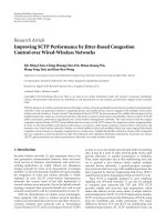
example, as Figure 1 shows, the 2.4 GHz band that 802.11 b/g
[3] standards operate on is split into eleven channels of
22 MHz-width, where the center frequencies of adjacent
channels are spaced by 5 MHz apart. So among the eleven
channels, only three are non-overlapped, namely, 1, 6, and
11. Due to the traditional static spectrum partition style,
almost all past research work assume channels of fixed
predetermined width. Recently some work [4–6] identified
the inefficiency of the static spectrum partition style and
began to explore the use of dynamic channel width adapta-
tion.
The aim of spectrum assignment is to distribute the
traffic load across the spectrum as evenly as possible. Fixed-
width channels can support uniformly distributed traffic
very well. But when the traffic distribution is skewed, the
use of fixed-width channels will be suboptimal and prohibit
the more effectively utilizing the spectrum resource. Let us

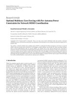
take Figure 2 as an example. Figure 2 shows a chain topology
where adjacent nodes are 200 m apart. Each node is assumed
to be equipped with two radio interfaces. The effective
transmission range is 250 m, and the interfering range is
550 m. The IEEE802.11 standard with RTS/CTS/DATA/ACK
four-way handshake is assumed to be used. So two links
within 3-hop range will conflict with each other when they
use the same channel.
2 EURASIP Journal on Wireless Communications and Networking
0
0.5
1
Normalised PSD
2400 2410 2420 2430 2440 2450 2460 2470
Frequency (MHz)
1
234567891011
Figure 1: Available eleven channels of fixed predetermined width defined in 802.11 b/g standards.
Each of the nodes from 1 to 9 is assumed to generate a
flow of same throughput U towards the gateway, node 10.
Intermediate nodes act as trafficgeneratorsaswellastraffic
routers at the same time. So different links carry different
trafficloads.InFigure 2(a), the number above each link
indicates the expected load on the link. For example, link
(5,6)hasaloadof5U since it forwards flows originating
from nodes 1 to 4 and the flow generated by node 5 itself.
Obviously, the bottleneck collision domain consists of links
(6, 7), (7, 8), (8, 9), and (9, 10), and hence limits the
throughput U for each flow.
We assume the total available spectrum is 60 MHz wide,

and each 1 MHz spectrum can deliver 1 Mbps data rate.
Here we consider static spectrum assignment scheme, that is,
channels are assigned to interfaces/links on a long-term basis.
In Figure 2(b), we first investigate the case that the whole
available spectrum is divided into three 20MHz-wide non-
overlapped channels. So at least two links among (6, 7), (7,
8), (8, 9), and (9, 10) will be assigned to the same channel.
As Figure 2(b) shows, the optimal scheme is to assign a
same channel to link (6, 7) and (7, 8), and assign the other
two channels to (8, 9) and (9, 10), respectively. Under this
scheme, links (6, 7) and (7, 8) become the bottleneck and
every flow can obtain the throughput U up to 20/13 Mbps.
In Figure 2(c), we then investigate another case that four
15 MHz-wide channels are available. Now no two links will
interfere with each other. Obviously, the bottleneck link is
(9, 10), and every flow can get the throughput U up to
5/3 Mbps, which is better than the previous case.
Note that flows could not benefit from the enhanced
capacity without first reducing the bottleneck wireless links.
By optimally adjusting channel width for every link, we
can get the most efficient spectrum assignment scheme as
Figure 2(d) shows. The spectrum that every link uses exactly
matches its traffic load. Now the throughput U for every
flow can get up to 2 Mbps. Compared with the previous two
fixed-width assignment schemes, channel width adaptation
can improve the network performance by 30% and 20%,
respectively.
Motivated by the above example, we strongly advocate
the channel width adaptable network architecture. Briefly
speaking, the advantages of channel width adaptation are

two-fold. On one hand, we can distribute the trafficas
evenly as possible across the spectrum in a fine granularity
to achieve channel load balance. On the other hand, in a
scenario with many interfering links, by “creating” more
small-width orthogonal channels, we can greatly reduce
the phenomena of contention and collision, and therefore
improve throughput as a result of fewer back-offsand
reduced interference. Another motivation for the channel
width adaptable network architecture is the recent open
spectrum effort [7] made by the spectrum regulation
authority such as FCC. Because of the variable widths of
“white space” unoccupied by licensed users, we believe
channel width adaptation will become one of the most
important functions for cognitive radio networks in future
open spectrum environment.
Thecharacteristicofwirelessmeshnetworks[1]makesit
attractive and feasible to use channel width adaptation. First,
in WMN, each mesh router aggregates trafficflowsforalarge
number of mobile clients, and therefore the aggregate traffic
load changes infrequently, which offers the predictability
for assigning channel width in term of traffic pattern and
permits capacity optimization based on estimated traffic
demand. Second, mesh nodes (or routers) are usually static
and have no power constraints, and therefore physical
topology changes only occur due to occasional node failures,
or addition of new nodes. Thus channel width adaptation
can be implemented on a long-term basis without requiring
resynchronization of interfaces for every packet. Third, some
mesh routers are used as gateways to connect the wired
network, and most traffic is between the mesh clients and

the wired networks through these gateways. So the traffic
distribution in WMN is typically skewed as the example in
Figure 2 shows: gateway nodes would form the bottlenecks
since more and more flows contend for the bandwidth as they
are forwarded closer to gateways. Channel width adaptation
will surely promise great flexibility to accommodate such
skewed traffi
c distribution.
In this paper, we address how to optimally adapt chan-
nel width in IEEE802.11-based multi-radio multi-channel
wireless mesh networks. We mathematically formulate the
channel width adaptation, logical topology design, and
routing as a joint optimization problem. Our mathematical
formulation not only takes into account the issues in
traditional MR-MC mesh networks, such as the number
of available interfaces, the interference constraints, and the
expected traffic load, but also determines at what center
frequency and how wide a spectrum band an interface
should use. Extensive simulations show that channel width
adaptation can significantly improve spectrum use efficiency
and network performance.
The rest of the paper is organized as follows. Section 2
reviews the related work. Section 3 presents the network
EURASIP Journal on Wireless Communications and Networking 3
12345678 9
1U 2U 3U 4U 5U 6U 7U 8U9U
10
(a) Chain topology.
12345678 9
CBAACBBAC

10
(b) Three 20 MHz-wide channels (A, B, C).
12345678 9
dcbadcbad
10
(c) Four 15 MHz-wide channels (a, b, c, d).
12345678 9
[42,60][26,42][12,26][0,12][50,60][42,50][36,42][32,36][30,32]
10
(d) Bandwidth adaptable channels.
Figure 2: Scenarios illustrating the inefficiency of using channels with fixed predetermined width. In Figure 2(d),aboveeachlink,[x, y]
denotes the frequency interval ranging from x MHz to y MHz which is assigned to that link.
model and Section 4 formulates the problem as a mixed
integer nonlinear programming. In Section 5,weconvert
the problem into an equivalent mixed 0–1 integer linear
programming and propose a suboptimal heuristic solution.
Simulation results are presented in Section 6,andSection 7
concludes this paper.
2. Related Work
There exists a wide range of related works aiming to
design efficient channel assignment algorithms for multi-
radio multi-channel mesh networks.
Raniwala proposed a static centralized channel assign-
ment algorithm in [8], and in [9], an improved distributed
channel assignment algorithm with load-balance routing
was proposed. In [10], channels are allocated so as to
minimize the maximum number of interfering links within
each neighborhood, subject to the constraint that the logical
topology graph should be K-connected. In [11], Kyasanur
and Vaidya proposed a hybrid channel assignment strategy,

easing the channel synchronization. Literature [12] proposed
a routing protocol which incorporates a routing metric
taking account of both the loss rate and the channel diversity
of links along the path. All the above algorithms are based on
heuristic methods, not mathematical formulations.
Many other works formulate the problem as a joint
mathematical programming. In [13], Alicherry et al. for-
mulated a joint channel assignment and routing problem
for the MR-MC network, with the aim of maximizing
network throughput subject to the proportional fairness
constraints. Literature [14] provided necessary conditions
of the feasibility of rate vectors and used a fast primal-
dual algorithm to derive upper bounds of the achievable
throughput. In [15], two models that maximize the number
of logical links that can be active simultaneously were
proposed, subject to interference constraints. In [16], the
MR-MC mesh architecture called TiMesh was proposed,
which formulates the logical topology control and interface
assignment as a joint optimization problem. All the above
works assume channels of fixed predetermined width.
Literature [17] proposed a spectrum sharing model for
cognitive radio networks based on mixed integer nonlinear
programming with the objective of minimizing the required
network-wide spectrum resource for a set of user sessions,
and developed a near-optimal algorithm based on the
sequential fixing procedure. It was mentioned in [17] that
equal band division of the spectrum yields suboptimal
performance and thus it calculated an optimal global band
partition. The significant difference between [17]andours
is that [17] only tries to obtain a global spectrum regulation

for the whole networks so that all nodes can use only one
spectrum partition style, while in our architecture we can
adjust channel width flexibly across nodes (i.e., different
nodes may use different spectrum partition styles), which
offers further flexibility.
Literature [4] first systematically studied the issues of
channel width adaptation. Using commodity 802.11 hard-
ware, it gave a method to generate signals of different
channel widths by changing the frequency of the reference
clock that drives the frequency synthesizer of the radio
front end circuitry, which can be configured dynamically
purely in software. And through detailed measurements
in controlled environments, it then preliminarily identified
several benefits of channel width adaptation in many met-
rics of wireless networks: range and connectivity, power
consumption, network capacity and fairness. Finally, it
proposed a channel width adaptation algorithm, called
SampleWidth, for two communicating nodes. In [5], three
centralized channel width adaptation algorithms using ILP,
LP-based packing and greedy raising were proposed for
WLAN to improve network capacity and per-client fair-
ness. Literature [6] designed a dynamic channel width
allocation protocol called b-SMART for cognitive radio
networks. Using the concept of time-spectrum block, the
spectrum allocation is reduced into the problem of pack-
ing time-spectrum blocks into a two-dimensional time-
frequency space. The algorithm of [6] resided in the
MAC layer and required advanced radio hardware with
fast switching and channel width adaptation ability on a
packet-by-packet basis, significantly increasing the signaling

4 EURASIP Journal on Wireless Communications and Networking
overhead due to the fast coordination. In our architecture,
channel width adaptation is on a long-term basis (e.g.,
every several minutes or hours), hence does not require
resynchronization of interfaces for every packet and the
modification of IEEE802.11 MAC protocols, and thus
becomes more practical for current available commercial
hardware and easy to be used in wireless backbone mesh
networks.
3. Network Model and Problem Formulation
We model the wireless mesh networks by an undirected
graph G(V, E), where V denotes the set of all vertices and E
denotes the set of all edges. Each vertex n
∈ V represents
a wireless mesh node equipped with K
n
network interface
cards, and we use n
p
to denote the pth interface of node n,
where p
= 1, 2, , K
n
.Foranytwonodes n, m ∈ V,ifnode
n is within the communication range of node m, then there
is a physical link (n, m)
∈ E between n and m. We assume
that all links are bidirectional.
Note that every node has multiple interfaces which can
be tuned into different portions of the spectrum, so there

may exist zero, one, or more logical links between two
neighboring nodes. Then based on the graph G,wedevelop
another radio-based graph G

(V

, E

), where V

={n
p
|
n ∈ V, p = 1, , K
n
} and E

={(n
p
, m
q
) | (n, m) ∈
E; p = 1, , K
n
; q = 1, , K
m
}. We call the links in E
physical links and the links in E

logical links. The logical link

(n
p
, m
q
) will exist in the final logical topology after spectrum
allocation if and only if the pth interface of node n and
the qth interface of node m operate on the same portion of
spectrum.
We assume that each interface can only be tuned into a
contiguous segment of the available spectrum. Due to the
hardware constraint, the possible channel widths are some
discrete values in the range of [b
min
, b
max
]. So it is reasonable
to partition the whole available spectrum into a series of
sequential small-width non-overlapped spectrum blocks. We
denote the set of blocks as F and the size of a spectrum
block as ω. So the problem of channel width adaptation
is equivalent to the contiguous spectrum blocks allocation.
For example, in Figure 2, we can set ω
= 2 MHz, and the
whole available 60 MHz-wide spectrum will be divided into
30 blocks. Link l
9,10
will be assigned the block 22 to block
30 and link l
8,9
will be assigned the block 14 to block 21 in

the scheme of Figure 2(d). According to Shannon’s capacity
theorem [18], we also reasonably assume that the achievable
data rate is proportional to the assigned channel width, that
is, the number of spectrum blocks allocated, and we let
c
unit
be the link-layer data rate that one spectrum block can
deliver.
We us e In f (n, m)
⊂ E to denote the set of physical
links that are in the interference range of link (n, m). Note
link (u, v)
∈ Inf (n, m) also indicates (n, m) ∈ Inf (u, v).
We assume that the non-overlapped spectrum bands are
orthogonal, that is, simultaneous use of non-overlapped
spectrum blocks in the same area will not interfere.
Though there may exist adjacent channel interference due
to improper signal processing at the wireless cards and
poor filter characteristics, we believe with the advance
of radio technology, adjacent channel interference can be
avoided to a large extent, and even partially overlapped
channels with variable width can be further exploited in the
future.
We assume that a reasonable statistical trafficdemand
matrix T is available. And let L
s,d
denote the trafficdemand
between the source and destination pair (s, d)
∈ T,
where s, d

∈ V. Our aim is to design schemes to maximize
the capacity of the network. The network capacity cannot
be simply measured by the total throughput of all traffic
flows. Optimizing such metric may lead to starvation of
some flows which originate far from gateways. We there-
fore need to consider some fairness constraints. Similar
to [13], we adopt the proportional fairness, that is, the
same portion of traffic demand will be satisfied for every
flow (s, d)
∈ T. So we want to find the schemes that
λL
s,d
trafficofeveryflow(s, d) ∈ T can be routed for
the largest possible λ. Other kinds of fairness constraint
like the lexicographical max-min fairness [19] can also be
adopted.
It is suboptimal to assigning spectrum without consider-
ing the logical topology control and traffic routing. So in our
work, the following three aspects will be jointly considered:
(1) logical topology design: which logical links in E

will
exist in the final topology?
(2) spectrum block assignment: how to efficiently assign
contiguous spectrum blocks to each interface?
(3) routing: how to optimally route the traffictoachieve
load balance across different links?
4. Joint Topology Design, Spectrum
Assignment, and Routing
In this section, we describe how we formulate the logical

topology design, contiguous spectrum block assignment,
and routing as a joint optimization problem. We will use the
letter like
l to denote a vector, and use l
i
to denote the ith
element of the vector
l.
4.1. Contiguous Spectrum Block Allocation. For any radio
interface n
p
of node n (n ∈ V, p = 1, , K
n
), we define
a
|F |×1 spectrum block assignment vector a
n
p
as follows:
a
i
n
p
=
⎧
⎨
⎩
1, if spectrum block i is assigned to radio n
p
,

0, otherwise,
(1)
where a
i
n
p
is the ith element of a
n
p
. For example, in
Figure 2(d), assuming node 9 uses its 2nd interface to
communicate with node 10, we have a
22
9
2
= a
23
9
2
=···=
a
30
9
2
= 1 while the other elements are equal to zero.
EURASIP Journal on Wireless Communications and Networking 5
a
n
p
[0, 0,1,1, ,1, 0, 0 ]

T
x
n
p
[0, 0,1,0, ,0, 0, 0 ]
T
y
n
p
[0, 0,0,0, ,1, 0, 0 ]
T
1234 ···
···
|F |
Frequency
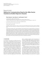
Figure 3: Illustration for vectors a
n
p
, x
n
p
,and y
n
p
.
In order to characterize the contiguous spectrum block
allocation, we then introduce two
|F |×1 auxiliary binary
vectors
x

n
p
and y
n
p
for a
n
p
as follows:
x
i
n
p
=
⎧
⎪
⎨
⎪
⎩
1, if a
i
n
p
= 1anda
j
n
p
= 0, j = 1, 2, , i − 1,
0, otherwise,
y

i
n
p
=
⎧
⎪
⎨
⎪
⎩
1, if a
i
n
p
= 1anda
j
n
p
= 0, j = i +1, , |F |,
0, otherwise.
(2)
Figure 3 illustrates a vector
a
n
p
and the corresponding
vectors
x
n
p
and y

n
p
. We can find the elements valued 1 of x
n
p
and y
n
p
indicate the lower and upper end of spectrum blocks
assigned to the radio interface n
p
, respectively. Obviously
every valid
a
n
p
corresponds to only one form of x
n
p
and y
n
p
.
x
n
p
and y
n
p
should satisfy

x
i
n
p
, y
i
n
p
∈{0, 1}, i = 1, 2, , |F |,
(3)
|F |

i=1
x
i
n
p
=
|F |

i=1
y
i
n
p
≤ 1, (4)
|F |

i=1
2

i
x
i
n
p
≤
|F |

i=1
2
i
y
i
n
p
,(5)
|F |

i=1
2
i
y
i
n
p
≤
|F |

i=1
2

i
x
i
n
p+1
,1≤ p ≤ K
n
−1. (6)
It is possible some radio interfaces do not take part in any
communication, so in this case, in constraint (4),

|F |
i=1
x
i
n
p
and

|F |
i=1
y
i
n
p
can be zero. Constraint (5) means that the lower
end of the spectrum segment should locate lower than the
upper end. And in constraint (6), without loss of generality,
we further assume that the spectrum segment that interface
n

p
uses locates lower than that of n
p+1
. Now using x
n
p
and
y
n
p
,wecanredefinea
n
p
as follows.
a
i
n
p
=
i

j=1
x
j
n
p
×
|F |

j=i

y
j
n
p
, i = 1, 2, , |F |. (7)
Which means for the element a
i
n
p
, if it resides between the
lower end and the upper end, it will be equal to 1, other-
wise 0.
When interface n
p
participates some communication, its
channel width should be in the range of [b
min
, b
max
], so the
total spectrum blocks that it can utilizes should be in the
range between b
min
/ω and b
max
/ω, that is,
b
min
ω
|F |


i=1
x
i
n
p
≤
|F |

i=1
a
i
n
p
≤
b
max
ω
|F |

i=1
x
i
n
p
. (8)
When we set b
min
= b
max

, our model will degenerate into the
traditional multi-radio multi-channel networks using fixed-
width channels.
Using the constraints (3)to(8), we can fully characterize
the contiguous spectrum block allocation. Note we can treat
a
n
p
as continuous real vectors since we can infer a
n
p
to be
binary vectors from the above constraints.
4.2. Logical Topology Formulation. Ve c t or s
x
n
p
and y
n
p
(thus
a
n
p
) can fully characterize the logical topology formulation.
The link (n
p
, m
q
) ∈ E


will exist in final logical topology
only when the interfaces n
p
and m
q
operate on the same set
of spectrum blocks. Then we use variable e
n
p
,m
q
to denote
whether the logical link (n
p
, m
q
) will exist, that is,
e
n
p
,m
q
=
⎧
⎨
⎩
1, if a
n
p

= a
m
q
,
0, otherwise.
(9)
We can alternatively express e
n
p
,m
q
as follows:
0
≤ 1 −e
n
p
,m
q
≤
|F |

i=1
a
i
n
p

a
i
m

p
, (10)
0
≤ e
n
p
,m
q
≤ 1 −a
i
n
p

a
i
m
q
i = 1, , |F |, (11)
where

is the exclusive OR (XOR) operator. It is easy to
verify the above correspondence. If there is some spectrum
block i that interface n
p
uses while m
q
does not or m
q
uses
while n

p
does not, that is, a
i
n
p

a
i
m
q
= 1, constraint (11)
will imply that e
n
p
,m
q
= 0. Otherwise, a
i
n
p

a
i
m
q
= 0for i =
1, , |F |, constraint (10) will imply that e
n
p
,m

q
= 1. Note
we can also treat e
n
p
,m
q
as continuous variables.
With e
n
p
,m
q
and a
n
p
, we can easily obtain the spectrum
assignment vector
a
n
p
,m
q
for any logical link (n
p
, m
q
) ∈ E

a

i
n
p
,m
q
= e
n
p
,m
q
×a
i
n
p

=
e
n
p
,m
q
×a
i
m
q

, i = 1, , |F |.
(12)
And the channel width that link (n
p

, m
q
)usesisequalto
ω

|F |
i=1
a
i
n
p
,m
q
.
4.3. Routing. In multihop WMNs, a source node may need
a number of relay nodes to route the data traffic towards its
destination node. We need to compute a network flow that
associates with each logical link (n
p
, m
q
) ∈ E

valued f
s,d
n
p
,m
q
,

where f
s,d
n
p
,m
q
denotes the traffic data rate for the source and
destination pair (s, d) that is being routed via the logical link
(n
p
, m
q
) in the direction from n
p
to m
q
, assuring the λ times
6 EURASIP Journal on Wireless Communications and Networking
of the trafficloadvaluedL
s,d
for every source and destination
pair (s, d)
∈ T can be routed.
The network flow should satisfy the following constraint:
for all n
∈ V,forall(s, d) ∈ T

m∈{v|(n,v)∈E}
K
n


p=1
K
m

q=1

f
s,d
n
p
,m
q
− f
s,d
m
q
,n
p

=
⎧
⎪
⎪
⎪
⎪
⎨
⎪
⎪
⎪

⎪
⎩
λL
s,d
,ifs = n,
−λL
s,d
,ifd = n,
0, otherwise,
(13)
which means if node n is the source of the flow, the net
flow sent by node n should be equal to λl
s,d
.Ifnoden is
the destination of the flow, it should be equal to
−λl
s,d
.For
the intermediate relay node, the net flow should be 0. Note
a feasible network flow also guarantees that the final logical
topology is connected.
The above constraint is only valid for the multi-path
routing, which can take advantage of load balancing. We
also investigate the single-path routing, which needs more
constraints besides (13). We define a binary routing variable
r
s,d
n
p
,m

q
for all (n
p
, m
q
) ∈ E

and for all (s,d) ∈ T. The variable
r
s,d
n
p
,m
q
will be equal to 1 if the flow from source s to destination
d is only routed via the logical link (n
p
, m
q
) in the direction
from n
p
to m
q
; otherwise it will be equal to 0. So r
s,d
n
p
,m
q

should
satisfy
r
s,d
n
p
,m
q
∈{0, 1}
, (14)

m∈{v|(n,v)∈E}
K
n

p=1
K
m

q=1
r
s,d
n
p
,m
q
≤1 ∀n∈V, ∀
(
s, d
)

∈ T, (15)
f
s,d
n
p
,m
q
= λr
s,d
n
p
,m
q
L
s,d
∀

n
p
, m
q

∈
E

. (16)
Constraint (15) ensures only one path exists between any
source and destination pair in T, and constraint (16)
guarantees that the flow will be routed along the path.
4.4. Interf erence Issues. For any two logical links (n

p
, m
q
) ∈
E

and (u
h
, v
l
) ∈ E

that (u, v) ∈ Inf (n, m), we define
interference indicator variable I
n
p
,m
q
,u
h
,v
l
as follows,
I
n
p
,m
q
,u
h

,v
l
=
⎧
⎨
⎩
1, if ∃i ∈{1, 2, , |F |}, a
i
n
p
,m
q
=a
i
u
h
,v
l
=1
0, otherwise
(17)
that is when these two logical links use overlapped spectrum
blocks, they will interfere with each other (I
n
p
,m
q
,u
h
,v

l
= 1).
Similar to the variable e
n
p
,m
q
, we can express the cor-
respondence among I
n
p
,m
q
,u
h
,v
l
, a
n
p
,m
q
and a
u
h
,v
l
with the
following constraints:
a

i
n
p
,m
q
×a
i
u
h
,v
l
≤ I
n
p
,m
q
,u
h
,v
l
≤ 1, i = 1, , |F |,
(18)
0
≤ I
n
p
,m
q
,u
h

,v
l
≤
|F |

i=1
a
i
n
p
,m
q
×a
i
u
h
,v
l
. (19)
4.5. Capacity Constraints. The fixed amount of spectrum
provides limited capacity that will be shared among the links
in interference range. First, we define a real variable u
n
p
,m
q
as
the link utilization for every logical links (n
p
, m

q
) ∈ E

, that
is, the fraction in one unit time that link (n
p
, m
q
)isactive.
Remember that we assume channel capacity is proportional
to the number of spectrum blocks it used. So u
n,m
should
satisfy the following constraints:
c
unit
|F |

i=1
a
i
n
p
,m
q
u
n
p
,m
q

=

(
s,d
)
∈T
f
s,d
n
p
,m
q
+

(
s,d
)
∈T
f
s,d
m
q
,n
p
,
(20)
0
≤ u
n
p

,m
q
≤ e
n
p
,m
q
. (21)
The term on right-hand side of constraint (20) is the
total traffic rate from all source and destination pairs that
is routed over link (n
p
, m
q
), which is equal to the link
utilization multiplies the channel capacity c
unit

|F |
i=1
a
i
n
p
,m
q
.
Since

|F |

i=1
a
i
n
p
,m
q
can be 0 (when the logical link does not
exist in the final logical topology, that is, e
n
p
,m
q
= 0), we use
constraint (21)tosetu
n
p
,m
q
to be 0 in that case.
Extending the sufficient condition for the existence of
inference-free schedule of [13], we have, for any (n
p
, m
q
) ∈
E

,
u

n
p
,m
q
+

(u,v)∈Inf (n,m)
K
u

h=1
K
v

l=1
u
u
h
,v
l
I
n
p
,m
q
,u
h
,v
l
≤ 1 (22)

which means that the total active time of logical link (n
p
, m
q
)
and all other interfering links in one unit time can not
exceed 1.
4.6. Objective Function. As stated before, our objective is to
find the largest possible λ, that is,
maximize λ. (23)
Now given the topology graph G(V, E), the parameters
ω, b
min
, b
max
, F , K
n
, c
unit
,andL
s,d
for all source and desti-
nation pairs in T, we can state our problem formally using
(3)-(23). However, note that many terms such as

i
j=1
x
j
n

p
×

|F |
j=i
y
j
n
p
in (7), a
i
n
p

a
i
m
q
in (10)and(11), and a
i
n
p
,m
q
u
n
p
,m
q
in (20) are nonlinear. Even relaxing the binary constraints of

(3)and(14), the problem is still nonconvex. So the above
programming is a mixed-integer nonconvex program and
generally it is not easy to be solved.
5. Solving the Problem
In this section, we first use some linearization techniques to
convert the original mixed-integer nonlinear programming
into a mixed-integer linear programming. Then we show
how to choose the optimal solution with least interference.
Finally we propose our heuristic MILP-based iterative local
search algorithms.
EURASIP Journal on Wireless Communications and Networking 7
5.1. Equivalent 0–1 Mixed-Integer Linear Programming.
Thanks to some binary linearization techniques [20, 21],
we can convert the above nonconvex programming into an
equivalent mixed integer linear programming. Tabl e 1 lists
three methods that will be used in our work. In the table,
the nonlinear constraint in column 1 can be equivalently
replaced by the corresponding linear constraints of column
3. These linearization techniques are also used in [22]for
partially overlapped channel assignment.
The validity of the above methods can be easily verified
by enumerating all possible combinations of θ
1
and θ
2
.
We ta ke τ
= θ
1


θ
2
as the example, where θ
1
and θ
2
are
two binary variables. When θ
1
= θ
2
= 0, the first linear
constraint θ
1
− θ
2
≤ τ will imply τ ≥ 0, and the third
linear constraint τ
≤ θ
1
+ θ
2
will imply τ ≤ 0, so we can
get τ
= 0. When θ
1
= 1, θ
2
= 0, or θ
1

= 0, θ
2
= 1, the
first/second constraints will imply τ
≥ 1, and the third and
the fourth constraints will imply τ
≤ 1, so τ = 1. Finally
when θ
1
= θ
2
= 1, the first and the second constraint will
imply τ
≥ 0, and the fourth constraint will imply τ ≤ 0, and
we can conclude that τ
= 0. So the four linear constraints are
exactly equivalent to the original nonlinear constraint. And
note we can treat τ as real variables. The other two methods
can be verified in the similar way.
In the original programming of Section 4,
x
n
p
, y
n
p
,
and r
s,d
n

p
,m
q
are explicitly declared binary vectors, while a
n
p
,
a
n
p
,m
q
, e
n
p
,m
q
and I
n
p
,m
q
,u
h
,v
l
can be directly or intermediately
implied to be binary vectors or binary variables from
x
n

p
and y
n
p
. u
n
p
,m
q
is a non-negative real variable with an
upper bound valued 1, and λ is also a non-negative real
variable upper bounded by
|F |c
unit
/L
s,d
. So it is possible for
us to convert all the nonlinear terms into linear ones. For
example, for the nonlinear term a
i
n
p

a
i
m
q
in (10)and(11),
we can first introduce auxiliary variables τ
i

n
p
,m
q
= a
i
n
p

a
i
m
q
for all (n
p
, m
q
) ∈ E

, i = 1, , |F |, and then replace
the constraint (10)and(11) with the linear constraints as
follows:
⎧
⎪
⎪
⎪
⎨
⎪
⎪
⎪

⎩
0 ≤ 1 − e
n
p
,m
q
≤
|F |

i=1
a
i
n
p

a
i
m
q
0 ≤ e
n
p
,m
q
≤ 1 −a
i
n
p

a

i
m
q
i = 1, , |F |
⇒
⎧
⎪
⎪
⎪
⎪
⎪
⎪
⎪
⎪
⎪
⎪
⎨
⎪
⎪
⎪
⎪
⎪
⎪
⎪
⎪
⎪
⎪
⎩
0 ≤ 1 − e
n

p
,m
q
≤
|F |

i=1
τ
i
n
p
,m
q
,
0
≤ e
n
p
,m
q
≤ 1 −τ
i
n
p
,m
q
, i = 1, , |F |,
a
i
n

p
−a
i
m
q
≤ τ
i
n
p
,m
q
≤ a
i
n
p
+ a
i
m
q
, i = 1, , |F |,
a
i
m
q
−a
i
n
p
≤ τ
i

n
p
,m
q
≤ 2 −a
i
n
p
−a
i
m
q
, i = 1, , |F |.
(24)
By applying the above three methods to convert all
nonlinear constraints into linear ones, we will get a mixed
0-1 integer linear programming (which is called as MILP-
1). The programming MILP-1 has 2
|F |

n∈v
K
n
binary
integer variables if we use multipath routing and additional
|T|

(n,m)∈E
K
n

K
m
binary integer variables if we use single
path routing. We can use the traditional branch-and-bound
algorithms [23] or use commercial software solver such as
LINDO [24] and CPLEX [25] to solve the problem.
5.2. The Optimal Scheme with Least Interference. The solu-
tion of programming MILP-1 is a spectrum assignment
scheme and a routing strategy that can maximize the value
of λ among all feasible solutions. However, MILP-1 may
produce sub-optimal solutions. We use Figure 4 to illustrate
it. Figure 4(a) shows a 5-node chain topology and each of
the nodes from 1 to 4 generates a flow of same throughput
U towards node 5. The number above each link indicates its
traffic load. The other assumptions are similar to Figure 2.
Figure 4(b) gives an optimal solution where the assigned
spectrum exactly matches each link’s traffic load and no two
links interfere with each other. However, the programming
MILP-1 may produce a solution like Figure 4(c) where
link (1, 2) and (4, 5) will share a same spectrum segment
[30 MHz, 60 MHz]. Under perfect time scheduler, both
schemes in Figure 4(b) and 4(c) can get a same throughput of
6 Mbps for every flow. However, when the contention-based
MAC technology like IEEE802.11 DCF is used, link (1, 2)
will interfere with link (4, 5) in the scheme of Figure 4(c),
causing some unnecessary contention and collision, and thus
decreasing the network performance. The reason why MILP-
1 may produce sub-optimal solution is that its constraints
are not able to take the cost of contention and collision into
consideration.

The above example suggests that we should select a
solution that can minimize interference from all solutions
which may be produced by MILP-1, that is, all solutions
attaining the same optimal λ valued of λ
∗
. First we adopt
following weighted metric to quantify the total interference.
To t
Inf
(
x,y, f ,λ
)
=

(n
p
,m
q
)∈E

⎧
⎨
⎩

(
s,d
)
∈T

f

s,d
n
p
,m
q
+ f
s,d
m
q
,n
p

·

(
u,v
)
∈Inf
(
n,m
)

h,l
I
n
p
,m
q
,u
h

,v
l
⎫
⎬
⎭
,
(25)
where

(s,d)∈T
( f
s,d
n
p
,m
q
+ f
s,d
m
q
,n
p
) is the total trafficoverlogical
link (n
p
, m
q
)and

(u,v)∈Inf(n,m)


h,l
I
n
p
,m
q
,u
h
,v
l
is the number
of other logical links interfering with (n
p
, m
q
).
Then we resolve the programming MILP-1 with the
modified goal of minimizing the metric Tot
inf with λ
fixed at λ
∗
, that is, we replace the constraint (13) with the
following equality

m∈{v|(n,v)∈E}
K
n

p=1

K
m

q=1

f
s,d
n
p
,m
q
− f
s,d
m
q
,n
p

=
⎧
⎪
⎪
⎪
⎨
⎪
⎪
⎪
⎩
λ
∗

L
s,d
,ifs = n,
−λ
∗
L
s,d
,ifd = n,
0, otherwise,
(26)
Note that the metric Tot
inf in (25) is nonlinear, but
we can easily linearize it via the techniques in Section 5.1
since I
n
p
,m
q
,u
h
,v
l
is an implied binary variable and f
s,d
m
q
,n
p
is a nonnegative real variable with upper bound λ
∗

l
s,d
.
Thus the new programming is still a mixed integer linear
programming. We call the modified programming MILP-2.
8 EURASIP Journal on Wireless Communications and Networking
Table 1: Binary linearization techniques.
Nonlinear constraint Variable Specification Equivalent linear constraints
π = θ
1
×θ
2
θ
1
, θ
2
∈{0, 1}
θ
1
+ θ
2
−π ≤ 1
0
≤ π ≤ θ
1
0 ≤ π ≤ θ
2
τ = θ
1
⊕θ

2
θ
1
, θ
2
∈{0, 1}
θ
1
−θ
2
≤ τ
θ
2
−θ
1
≤ τ
τ
≤ θ
1
+ θ
2
τ ≤ 2 −θ
1
−θ
2
σ =r ×θ
1
θ
1
∈{0, 1}, 0 ≤ σ ≤r

max
θ
1
r ∈ R, and r
max
(θ
1
−1) + r ≤ σ
0
≤ r ≤ r
max
σ ≤r
max
(1 −θ
1
)+r
12345
1U 2U 3U 4U
(a) 5-node chain topology.
12345
[36,60][12,30][0,12][30,36]
(b) An optimal solution.
12345
[30,60][12,30][0,12][30,60]
(c) A suboptimal solution which may be produced by MILP-1.
Figure 4: MILP-1 may produce suboptimal solution. We still assume that the total available spectrum is 60MHz wide and each 1 MHz
spectrum can deliver 1 Mbps data rate. Under perfect time scheduler, both schemes in Figures 4(b) and 4(c) can obtain the same throughput
U of 6Mbps for every flow. But in the scheme of Figure 4(c), link (1, 2) interferes with link (4, 5). When the contention-based MAC
technology is used, it may cause unnecessary contention and collision.
5.3. Heuristic MILP-based Iterative Local Search Algorithm. It

is well known that the computational complexity of a mixed
integer linear programming mainly depends on the number
of integer variables [23]. So for large-scale networks, it will
not be trivial to find the optimal solutions to MILP-1 and
MILP-2. So we need to make some tradeoff between the
performance improvement and computation complexity. In
this section, we present our heuristic suboptimal algorithm.
Our heuristic algorithm is an iterative local search
algorithms [26] in which the basic idea is to start with
an initial feasible solution and then make modifications to
improve its quality using the original MILP. In this section,
we only assume that the multipath routing is used, and all
nodes are equipped with same K interfaces.
We initially partition the whole available spectrum into K
segments with approximately same size. Then we will assign
the first b
max
/ω spectrum blocks of each segment to the
interfaces of every node. For example, if we have 30 spectrum
blocks, and K
= 3, b
max
/ω = 6, we will assign blocks 1-
6, blocks 11–16, and blocks 21–26 to the first, second and
third interface of every node, respectively. Obviously, the
network is full connected and only the logic links in the set
{(n
i
, m
i

)|(n, m) ∈ E, i = 1, , K} are preserved.
Then we run the programming MILP-1 on the full con-
nected networks under the given initial spectrum assignment
to obtain an initial load balance routing. Note here that
MILP-1 becomes a linear programming. With the initial
spectrum assignment and routing, we will iterate to create
a sequence of solutions in an attempt to gradually improve
the network performance.
In iteration i, we first sort all logical links (n
p
, m
q
) in the
decreasing order of the following congestion metric:
Cong

n
p
, m
q

=
u
n
p
,m
q
+

(

u,v
)
∈Inf
(
n,m
)

h,l
u
u
h
,v
l
I
n
p
,m
q
,u
h
,v
l
,
(27)
which is the term on the left-hand side of constraint (22),
denoting the congestion status of the collision domain
centered at the logical link (n
p
, m
q

).
We should adopt some randomness to escape from the
local optimum. So then we randomly choose a logical link
(n
p
, m
q
) from the L most congested links and try to adjust the
spectrum allocation of all interfaces in the interference range
of nodes n and m. The adjustment is conducted by running a
modified version of MILP-1 and MILP-2, where the variables
are only a subset of variables of the original problem,
while the values of others are kept as constant as those in
the previous iteration. Note only that the variables
x, y, f ,
and λ are what we concern about while others are only
intermediate variables. For any radio interface u
h
where ∃v ∈
V that (u, v) ∈ Inf (n, m), we mark x
u
h
, y
u
h
as variables of
the new iteration. We also mark f
s,d
u
h

,v
l
for all (u
h
, v
l
) ∈ E

,
for all (s, d)
∈ T to be variables. The modified problem has
much fewer integer variables than the original one, so we
can solve it easily by branch-and-bound algorithm. It can be
viewed as the local search process.
The iteration will terminate when a maximum number
(i
max
) of allowed iterations have passed without improve-
ment. In our algorithms, we set i
max
to 2|E|.Abrief
description of our algorithms is shown in Algorithm 1.
EURASIP Journal on Wireless Communications and Networking 9
Input: G(V, E), b
min
, b
max
, ω,F , K,c
unit
Output: spectrum allocation x, y and routing f

BEGIN
1. Partition the whole available spectrum into K segments with approximately same size.
2. Assign the first b
max
/ω spectrum blocks of each segment to the interfaces of every node.
3. Run the programming MILP-1 on the full connected networks under the given initial spectrum
assignment to obtain an initial load balance routing, initial λ
(0)
and Tot inf
(0)
.
4. i
= 0,j = 1.
5. WHILE i
≤ i
max
DO
(a) Sort logical links (n
p
, m
q
) ∈ E

in the decreasing order of the metric Cong(n
p
, m
q
)
(b) Randomly choose a logical link (n
p

, m
q
)fromtheL most congested links
(c) Solve the modified programming MILP-1 with the following variables:
{x
u
h
, y
u
h
|∃v (u, v) ∈ Inf (n, m)}∪{f
s,d
u
h
,v
l
(u
h
, v
l
) ∈ E

,(s,d) ∈ T}∪{λ}
while the values of others are kept as constant as in previous iteration. The new objective
value of MILP-1 is λ
(j)
.
(d) Solve the modified programming MILP-2 with the same set of variables as in step 5(c) while
the value of λ is fixed at λ
(j)

, and get the new value of total interference Tot inf
(j)
(e) IF λ
(j)
= λ
(j−1)
&& Tot inf
(j)
= Tot inf
(j−1)
i = i +1.
END IF
(f) j
= j +1
END WHILE
END
Algorithm 1: MILP-based Heuristic Iterative Local Search Algorithms.
6. Performance Evaluation
In this section, we compare the performance of our proposed
channel width adaptable network architecture with the
traditional multi-radio multi-channel networks using fixed-
width channels. We also discuss the impact of some system
parameters on the network performance.
The simulation is conducted by NS-2 simulator [27]. We
use the methods described in [28] to add multi-interface
support and extend the channel module to enable channel
width adaptation. The following are the default settings for
simulation. We use IEEE802.11 DCF as the MAC layer, and
RTS/CTS mechanism is enabled. The two-ray propagation
model is used to model the path loss. The transmission

range is set to be 250 m, and the interference range is 550 m.
The total available spectrum is assumed to be 120 MHz-
wide, and each node is equipped with three interfaces. For
our channel width adaptable architecture, we set the default
spectrum block size ω to be 5 MHz, and set b
min
and b
max
to be 5 MHz and 50 MHz respectively. The default routing
scheme is multi-path routing. In our implementation of the
multipath routing in NS-2, every node forwards data packets
across different links with the probability proportional to the
routing flows calculated by our programming.
6.1. Optimal and Suboptimal Solutions on Grid Topology. We
first present the results obtained by the optimal branch-
and-cut solver [25] and our heuristic MILP-based iterative
local search algorithm on the 6
× 6gridtopology.We
also investigate the performance of MR-MC networks using
fixed-width channels, whose solution can be obtained from
our MILP programming by adding the constraint b
min
=
b
max
= 20MHz. We repeat our simulation on the 6 × 6grid
topology for 10 randomly generated trafficprofiles.Ineach
profile, we randomly chose twelve source and destination
node pairs to generate UDP (User Datagram Protocol)
sessions. Each has the transmission demand uniformly

distributed between 1 Mbps and 5 Mbps. Then we change
every flow’s rate proportionally until the network can satisfy
90% of the injected traffic. The metric we examine is the total
useful throughput across all sessions.
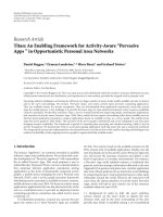
Figure 5 shows the total useful throughput obtained
by the optimal solution, our heuristic solution, and the
case using fixed-width channels. It shows that in the grid
topology, the optimal solution can outperform the case using
fixed-width channels by 32% on average while our heuristic
algorithm can improve the performance by 24% on average.
The performance gap between the optimal solution and our
heuristic solution is about 8%.
6.2. Comparison with “Hyacinth” Architecture. “Hyacinth”
is a typical MR-MC mesh networks. A static centralized
fixed-width channel assignment algorithm for “Hyacinth”
architecture is proposed in [8]. With the assumption that
most traffic is between the mesh clients and the gateway
nodes, it first estimates the total expected load on each
virtual link by summing the load due to each offered traffic
flow. Then, the channel assignment algorithm visits each
virtual link in decreasing order of expected trafficloadand
greedily assigns it a channel. In this subsection, we compare
the performance of our heuristic channel-width adaptation
algorithm with the typical WMN architecture “Hyacinth.”
In “Hyacinth” architecture, we want to study the impact
10 EURASIP Journal on Wireless Communications and Networking
15
20
25
30

35
40
Network useful throughput (Mbps)
12345678910
Tr affic profile index
Fixed-width channels
Heuristic solution
Optimal solution
Figure 5: Comparison on the total useful throughput of the optimal
solution and heuristic solution across 10 traffic profiles.
of different static spectrum partition styles. Specifically,
three cases are investigated: (1) The 120 MHz-wide available
spectrum is divided into twelve 10 MHz-wide channels.
(2) Six 20 MHz-wide channels and (3) Four 30 MHz-wide
channels.
The simulation scenario is an area of 1000 m
×1000 m
consisting of 40 randomly located mesh nodes. Among the 40
nodes, 3 nodes are randomly chosen to act as gateways and 15
nodes are chosen to generate UDP traffic flows towards one
of these gateway nodes. The initial rate of traffic flow is also
uniformly selected between 1 Mbps and 5 Mbps. Remaining
nodes only act as traffic routers. We proportionally change
every flow’s rate until the network can satisfy 90% of the
traffic. In this subsection, both the “Hyacinth” architecture
and our algorithms adopt the single-path routing.
Figure 6 shows the total useful throughput of the above
three static spectrum partition styles and our heuristic
algorithm in twenty randomly generated topologies. The
case of 12

× 10 MHz-wide channels usually performs the
worst since the number of interfaces constraints the maximal
spectrum resource that a node can utilize. In this case, even
though all interfaces are saturated, some portion of the
spectrum is still not utilized. For the case of 4
× 30 MHz-
wide channels and the case of 6
× 20 MHz-wide channels,
we find that no one can dominate the other across all
topologies because different topologies and trafficprofiles
give different preferences to spectrum partition styles. By
adjusting channel width to cater to different topology and
traffic demand, our scheme always outperforms the others
and get an improved total throughput by 18% to 46%
compared with the cases of 4
×30 MHz and 6×20 MHz. Note
the performance improvements are achieved without using
extra spectrum resources. Thus, the spectrum is utilized
more efficiently in our architecture. The key reason is that
we can distribute the load across the spectrum as evenly
as possible, and links can share the spectrum resource in
a much fairer way than in static spectrum partition styles.
And by creating many small-width channels, the phenomena
10
15
20
25
30
35
40

45
Network useful throughput (Mbps)
1 2 3 4 5 6 7 8 9 1011121314151617181920
Topology sample index
12
×10Mhz
4
×30Mhz
6
×20Mhz
Channel width adaptation
Figure 6: Comparison on the total useful throughput between
Hyacinth and our algorithm across 20 randomly generated topolo-
gies.
of collision, contention, and interference among links can
be significantly reduced or even eliminated, and thus the
performance is further improved.
6.3. The Impact of Spectrum Block Size. The most important
system parameter in our algorithms is the size of spectrum
block ω. With small spectrum block size, we can adjust
channel width in a finer granularity and it is possible to
obtain more performance improvement. However, using too
small spectrum block size will incur significant hardware
cost and computation complexity. In this subsection we
investigate the impact of spectrum block size ω on the
network performance.
The simulation scenario is similar to that of Section 6.2.
We vary the spectrum block size ω from 1 MHz to 15 MHz.
The MR-MC networks using 6
× 20 MHz-wide channels is

used as the comparison baseline. Figure 7 shows the relative
performance gains under different spectrum block size. Each
point is the average of measurements for twenty randomly
generated topologies. Generally speaking, the performance
gain is increased as the spectrum block size becomes small.
But when the spectrum block size ω
≥ 10 MHz, there is
nearly no improvement compared with the case using fixed-
width channels. And when ω<4 MHz, the improvement
due to using much smaller spectrum block will become
unremarkable. So some tradeoff shouldbemadebetween
the hardware complexity and performance improvement. We
may think 5 MHz is the most appropriate spectrum block size
for our simulation scenario.
6.4. The Impact of Routing Scheme. In this subsection, we
investigate the impact of routing scheme on the network
performance with or without channel width adaptation.
Specifically, four cases are investigated: Multi-path routing
combined with Fixed-width Channels (MP-FC), Multi-
path routing with channel Width Adaptation (MP-WA),
Single-path routing with Fixed-width Channels (SP-FC),
EURASIP Journal on Wireless Communications and Networking 11
0.9
1
1.1
1.2
1.3
1.4
1.5
Relative performance gains

123456789101112131415
Spectrum block size (Mhz)
Figure 7: Comparison of the performance gains under different
spectrum block size.
20
25
30
35
40
45
Network useful throughput (Mbps)
12345678910
Topology sample index
SP-FC
SP-WA
MP-FC
MP-WA
Figure 8: Comparison on the total useful throughput under
different routing schemes across 10 randomly generated topologies.
25
30
35
40
45
50
Network useful throughput (Mbps)
12345678
Topology sample index
Num
interface = 3

Num
interface = 6
Num
interface = 4
Num
interface = 7
Num
interface = 5
Figure 9: Comparison on the total useful throughput using differ-
ent number of interfaces across 8 randomly generated topologies.
and Single-path routing with channel Width Adaptation
(SP-WA). For the cases of fixed-width channels, the
whole available spectrum is divided into six 20 MHz-wide
non-overlapped channels. Figure 8 shows the total useful
throughput for the four cases across ten randomly generated
topologies.Aswecanexpect,SP-FCusuallyperformsworst
while MP-WA always performs best. And for the cases of
MP-FC and SP-WA, no one can dominate the other across
all topologies. Actually multipath routing and channel width
adaptation are complementary to each other. Multi-path
routing takes advantage of load balancing across links, while
channel width adaptation can distribute the load more evenly
across spectrum.
6.5. The Impact of Number of Interfaces per Node. In multi-
radio multi-channel mesh networks using fixed-width chan-
nels, there is no need to equip each node with more interfaces
than the number of channels. However, with the ability of
channel width adaptation, we can benefit from equipping
more interfaces in our architecture. Figure 9 shows the
effect of varying number of interfaces per node on network

throughput. The useful throughput increases monotonically
with the number of interfaces. And even when the number
of interfaces exceeds 6, some performance gains still can be
obtained, though at this time the values of λ calculated in
our programming are almost same (note that the values of
λ indicates the upper bound of the network capacity). This
is because with more interfaces, it is possible to create more
small-width channels, thus reducing interference among
links and saving the spectrum resource from contention
and collision. It can also mitigate the problem of spectrum
overfragmentation and thus the spectrum can be more
efficiently utilized.
7. Conclusion
In this paper, we address how to adapt channel width
to make full use of the spectrum resource in multi-radio
multi-channel wireless mesh networks. We mathematically
formulate the channel width adaptation, topology control
and routing as the mixed 0-1 integer linear optimization. We
also propose a heuristic assignment algorithm. Simulation
results show that our algorithm can significantly improve
spectrum use efficiency and network performance.
Our work distinguishes from prior optimization works
in that it does not treat the spectrum as the set of discrete
orthogonal channels but the continuous resource. The com-
bination of variable channel widths and center frequencies
offers rich possibilities for improving system performance. A
lot of things still need to be done. Currently, we are exploiting
the partially overlapped channels with adaptable widths in
our model to further improve the spectrum efficiency.
References

[1] I. F. Akyildiz, X. Wang, and W. Wang, “Wireless mesh
networks: a survey,” Computer Networks,vol.47,no.4,pp.
445–487, 2005.
12 EURASIP Journal on Wireless Communications and Networking
[2] P. Gupta and P. R. Kumar, “The capacity of wireless networks,”
IEEE Transactions on Information Theory,vol.46,no.2,pp.
388–404, 2000.
[3] IEEE 802.11b Standard, />802.11.html.
[4] R. Chandra, R. Mahajan, T. Moscibroda, R. Raghavendra,
and P. Bahl, “A case for adapting channel width in wireless
networks,” in Proceedings of the ACM SIGCOMM Conference
on Data Communication, pp. 135–146, Seattle, Wash, USA,
August 2008.
[5] T. Moscibroda, R. Chandra, Y. Wu, S. Sengupta, P. Bahl,
and Y. Yuan, “Load-aware spectrum distribution in wireless
LANs,” in IEEE International Conference on Network Protocols
(ICNP ’08), pp. 137–146, Orlando, Fla, USA, October 2008.
[6] Y. Yuan, P. Bahl, R. Chandra, T. Moscibroda, and Y. Wu,
“Allocating dynamic time-spectrum blocks in cognitive radio
networks,” in Proceedings of the 8th ACM International
Symposium on Mobile Ad Hoc Networking and Computing
(MobiHoc ’07), pp. 130–139, Montreal, Canada, September
2007.
[7] I.F.Akyildiz,W Y.Lee,M.C.Vuran,andS.Mohanty,“NeXt
generation/dynamic spectrum access/cognitive radio wireless
networks: a survey,” Computer Networks, vol. 50, no. 13, pp.
2127–2159, 2006.
[8] A. Raniwala, K. Gopalan, and T. Chiueh, “Centralized channel
assignment and routing algorithms for multi-channel wireless
mesh networks,” ACM SIGMOBILE Mobile Computing and

Communications Re view, vol. 8, no. 2, pp. 50–65, 2004.
[9] A. Raniwala and T C. Chiueh, “Architecture and algorithms
for an IEEE 802.11-based multi-channel wireless mesh net-
work,” in Proceedings of the 24th IEEE Annual Joint Conference
of the IEEE Computer and Communications Societies (INFO-
COM ’05), vol. 3, pp. 2223–2234, Miami, Fla, USA, March
2005.
[10] J. Tang, G. Xue, and W. Zhang, “Interference-aware topology
control and QoS routing in multi-channel wireless mesh net-
works,” in Proceedings of the 6th ACM International Symposium
on Mobile Ad Hoc Networking and Computing (MobiHoc ’05),
pp. 68–77, Urbana-Champaign, Ill, USA, May 2005.
[11] P. Kyasanur and N. H. Vaidya, “Routing and interface assign-
ment in multi-channel multi-interface wireless networks,”
in Proceedings of the IEEE Wireless Communications and
Networking Conference (WCNC ’05), vol. 4, pp. 2051–2056,
New Orleans, La, USA, March 2005.
[12] R. Draves, J. Padhye, and B. Zill, “Routing in multi-radio,
multi-hop wireless mesh networks,” in Proceedings of the 10th
Annual International Conference on Mobile Computing and
Networking (MOBICOM ’04), pp. 114–128, Philadelphia, Pa,
USA, September 2004.
[13] M. Alicherry, R. Bhatia, and L. Li, “Joint channel assignment
and routing for throughput optimization in multi-radio
wireless mesh networks,” in Proceedings of the 11th Annual
International Conference on Mobile Computing and Networking
(MOBICOM ’05), pp. 58–72, Cologne, Germany, August-
September 2005.
[14] M. Kodialam and T. Nandagopal, “Characterizing the capacity
region in multi-radio multi-channel wireless mesh networks,”

in Proceedings of the 11th Annual International Conference on
Mobile Computing and Networking (MOBICOM ’05), pp. 73–
87, Cologne, Germany, August-September 2005.
[15] A. K. Das, H. M. K. Alazemi, R. Vijayakumar, and S. Roy,
“Optimization models for fixed channel assignment in wire-
less mesh networks with multiple radios,” in Proceedings of the
2nd Annual IEEE Communications Society Conference on Sen-
sor and AdHoc Communications and Networks (SECON ’05),
pp. 463–474, Santa Clara, Calif, USA, September 2005.
[16] A. H. M. Rad and V. W. S. Wong, “WSN16-4: logical
topology design and interface assignment for multi-channel
wireless mesh networks,” in Proceedings of the IEEE Global
Telecommunications Conference (GLOBECOM ’06), pp. 1–6,
San Francisco, Calif, USA, November-December 2006.
[17] Y. T. Hou, Y. Shi, and H. D. Sherali, “Optimal spectrum
sharing for multi-hop software defined radio networks,” in
Proceedings of the 26th IEEE Annual Joint Conference of
the IEEE Computer and Communications Societies (INFO-
COM ’07), pp. 1–9, Anchorage, Alaska, USA, May 2007.
[18] T. M. Cover and J. A. Thomas, Elements of Information Theory,
John Wiley & Sons, New York, NY, USA, 1991.
[19] J. Tang, G. Xue, and W. Zhang, “Maximum throughput and
fair bandwidth allocation in multi-channel wireless mesh net-
works,” in Proceedings of the 25th IEEE Conference on Computer
Communications (INFOCOM ’06), pp. 1–10, Barcelona, Spain,
April 2006.
[20] F. Glover and E. Woolsey, “Further reduction of zero-
one polynomial programming problems to zero-one linear
programming,” Operations Research, vol. 21, no. 1, pp. 156–
161, 1973.

[21] C T. Chang and C C. Chang, “A linearization method for
mixed 0-1 polynomial programs,” Computers & Operations
Research, vol. 27, no. 10, pp. 1005–1016, 2000.
[22] A. H. M. Rad and V.W. S. Wong, “Partially overlapped channel
assignment for multi-channel wireless mesh networks,” in
Proceedings of the IEEE International Conference on Commu-
nications (ICC ’07), pp. 3770–3775, Glasgow, UK, June 2007.
[23] S. G. Nash and A. Sofer, Linear and Nonlinear Programming,
McGraw-Hill, Boston, Mass, USA, 1996.
[24] “LINDO MILP solver,” .
[25] ILOG CPLEX, />[26]H.R.Lourenco,O.Martin,andT.Stutzle,“Iteratedlocal
search,” in Handbook of Metaheuristics,F.GloverandG.
Kochenberger, Eds., pp. 321–353, Kluwer Academic Publish-
ers, Dordrecht, The Netherlands, 2002.
[27] UCB/LBNL/VINT, “Network Simulator (ns), version 2,” http:
//www.isi.edu/nsnam/ns.
[28] R. A. Calvo and J. P. Campo, “Adding Multiple Interface
Support in NS-2,” January 2007, />aguerocr/files/ucMultiIfacesSupport.pdf.