Báo cáo hóa học: " Research Article An Efficient Addressing Scheme and Its Routing Algorithm for a Large-Scale Wireless Sensor Network" pptx
Bạn đang xem bản rút gọn của tài liệu. Xem và tải ngay bản đầy đủ của tài liệu tại đây (947.72 KB, 13 trang )
Hindawi Publishing Corporation
EURASIP Journal on Wireless Communications and Networking
Volume 2008, Article ID 765803, 13 pages
doi:10.1155/2008/765803
Research Article
An Efficient Addressing Scheme and Its Routing Algorithm for
a Large-Scale Wireless Sensor Network
Soojung Hur,
1
Jaehyen Kim,
1
Jeonghee Choi,
2
and Yongwan Park
1
1
Mobile Communication Laboratory, Yeungnam University, Gyeongsan, Gyeogbuk 712-749, South Korea
2
School of Computer Communication Engineering, Daegu University, Gyeongsan, Gyeongbuk 712-714, South Korea
Correspondence should be addressed to Yongwan Park,
Received 31 December 2007; Revised 5 June 2008; Accepted 22 September 2008
Recommended by Athanasios Vasilakos
So far, various addressing and routing algorithms have been extensively studied for wireless sensor networks (WSNs), but many
of them were limited to cover less than hundreds of sensor nodes. It is largely due to stringent requirements for fully distributed
coordination among sensor nodes, leading to the wasteful use of available address space. As there is a growing need for a large-
scale WSN, it will be extremely challenging to support more than thousands of nodes, using existing standard bodies. Moreover,
it is highly unlikely to change the existing standards, primarily due to backward compatibility issue. In response, we propose an
elegant addressing scheme and its routing algorithm. While maintaining the existing address scheme, it tackles the wastage problem
and achieves no additional memory storage during a routing. We also present an adaptive routing algorithm for location-aware
applications, using our addressing scheme. Through a series of simulations, we prove that our approach can achieve two times
lesser routing time than the existing standard in a ZigBee network.
Copyright © 2008 Soojung Hur et al. This is an open access article distributed under the Creative Commons Attribution License,
which permits unrestricted use, distribution, and reproduction in any medium, provided the original work is properly cited.
1. INTRODUCTION
Large-scale events such as disaster relief or rescue efforts
require the most effective and highly available communi-
cation capabilities. To provide better communication and
monitoring capabilities, such applications may be tremen-
dously benefited from the use of self-organizing networks
over wireless medium [1]. Existing wireless sensor networks
(WSNs) such as ZigBee network, however, do not scale well,
because many of them have targeted smaller deployments,
typically less than hundreds of sensors. Real world deploy-
ments identified several limitations in the existing WSNs and
reported that certain physical topologies would run out of
address space quickly [2].
We recognized that such limitations were closely related
with the addressing schemes and the routing methods of
WSN standards. To uniquely identify sensor nodes through
their addresses in an ad hoc and mesh-style wireless network,
standard address schemes such as ZigBee Cskip algorithm
[3] utilize available address space sparsely, thus causing
significant wastage of address space [2, 4, 5]. In a large-scale
WSN, flat routing methods are unsuitable because of their
flooding nature for routing path construction [6–8]. On the
other hand, tree-based routing methods, at the expense of
robustness, achieve acceptable routing performance because
of their low routing overhead [9, 10].
In this study, we focus on an efficient address assignment
scheme by using n-dimensional address subspacing and
its tree-based routing algorithm for a large-scale WSN.
Especially, we are interested in tackling the address wastage
problem for a ZigBee network. We also present a location-
aware routing algorithm that also uses our address subspac-
ing and discuss its pros and cons.
This article is organized as follows. In Section 2,various
addressing assignment schemes and their routing algorithms
are presented. Section 3 introduces the addressing scheme
and its routing policy of early ZigBee standard, addresses
itsproblem,andreportsseveralproposalstocopewith
the problem. In Section 4,wedescribeourn-dimensional
addressing scheme and its routing algorithm that reuses
the existing address scheme. In the same section, we also
discuss the potential of the location-aware routing algorithm
that is also newly devised to improve wireless performance.
Section 5 reports the evaluation results of existing addressing
2 EURASIP Journal on Wireless Communications and Networking
scheme and our scheme through simulations. Finally, we
describe our contributions and future research direction in
Section 6.
2. RELATED WORKS
Addressing and routing have been extensively studied in
the literature for decades. It will be too ambitious to cover
all the issues in rather a short section. Instead, we present
general ideas and trends in these areas for WSNs. For a better
presentation, we separate issues into two parts: addressing
and routing.
2.1. Addressing
Existing addressing policies in WSNs fall into two groups:
tree based and ad hoc based. The tree-based addressing uses
hierarchical addressing policy [11, 12], while the ad hoc
addressing is originated from the addressing schemes for
wireless ad hoc network [13–15].
PalChaudhuri et al. proposed a robust, stateless address-
ing, and routing architecture called TreeCast [11]. Unlike
what the name implies, its address assignment is the most
crucial step, while its routing procedure is trivial. It is because
the address of a newly joining node is determined on demand
and the address in itself encapsulates the path to a parent.
Therefore, routing from a source to a sink becomes trivial.
A new node joins the network by choosing its parent among
candidate parents randomly. Its new address is incrementally
allocated by combining the parent address with a locally
unique identifier. However, its addressing scheme is only
optimized for a single sink node. To support multiple sink
nodes, the algorithm requires multiple addresses per node,
each of which is originated from individual sink node.
Thus, it is useless for the applications that use end-to-end
communication between two arbitrary nodes.
Huynh and Hong suggested a hybrid architecture that
has both hierarchical and mesh-style routing features [12].
Firstly, it is a layered architecture. Every sensor node should
reside in one of the layers and needs a unique parent in
its above layer, maintaining a hierarchical structure. Once
a parent node is chosen, TreeCast-like incremental address
assignment is applied, that is, the address of a newly joined
node includes its parent address. Therefore, a node in a
higher layer always has a smaller address length than other
node in a lower layer. Secondly, every node residing in the
same layer is interconnected with each other in the form of a
de Bruijn graph, a special case of mesh structure. Therefore,
if a source and a destination have the same address length,
intralayer routing along mesh topology will be performed.
Otherwise, interlayer routing along tree topology would
then be firstly executed. While it allows arbitrary end-to-
end communication, its applicability is limited to indoor
applications, where all sensor nodes are immovable.
The naive address assignment policy is to use a central-
ized scheme, where a single server in a network is dedicated
to assign addresses for a new node with no conflict. As long
as the server operates, uniqueness of allocated addresses is
guaranteed. In spite of its simple design, a single-point-of-
failure problem has been the biggest obstacle in its popular
use in ad hoc environments. In a decentralized addressing
scheme, each node configures its address and then announces
the address through flooding mechanism [13]. If any address
conflict is detected, all the other nodes in the network
will negotiate to resolve the address conflict to validate the
uniqueness of the address through global agreement.
IPAA [14] adopts a trial and error policy to find an
available IP address for a new node [14]. A new node
selects two random IP addresses from the IP address block,
which is divided into two categories, a temporary address
for duplicate address detection (DAD) and the actual address
to use for communication. The node then creates a dummy
message with the source address of the temporary IP that
inquires whether the address is used by any other and floods
it to the network. If there is no reply during a given period,
the node will consider that it is free and thus will take the
address as its own address. Otherwise, it selects another
address and iterates the previous procedures again until any
free address is found.
In the token-based scheme, a special node is assigned to
a token holder, which takes in charge of address allocation
for a new node [15]. Similar to the centralized scheme, a
new node contacts the token holder to get a unique address.
However, every node in the network should keep track of the
latest address of the holder.
2.2. Routing methods
Current routing protocols for WSNs can be grouped into two
categories: flat routing [6–8] and hierarchical routing [9, 10].
The flat routing assumes that every node runs the same
communication strategy and collaborates the forwarding
of data packets toward a sink node with other nodes. In
this routing, there is no discrimination on the routing role
among sensors. The hierarchical routing, however, imposes
a special mission on specially chosen nodes (i.e., cluster
headers). Cluster headers collect newly generated packets
from noncluster header nodes, aggregate them, and forward
them to a sink node. To do so, the cluster headers operate
continuously with no idle time, thus consuming more energy
than ordinary nodes.
Directed diffusion is a new paradigm that shifted our
attention from node-centric routing to data-centric routing
[6]. Figure 1 illustrates the schematic view of its three steps.
First, a sink node sends its interest to sensors, using flooding
(interest propagation). Next, every intermediate node sets
up communication paths from a source to a sink, allowing
multiple paths (gradients setup). Finally, an optimal path
such as lowest-delay path among the multiple paths is chosen
to deliver data efficiently (reinforcement).
Energy-aware routing aimed to increase the survivability
of networks [8]. The basic idea is that it maintains multiple
paths from a source to a sink and uses one path among
them randomly and probabilistically. It is similar to directed
diffusion in that they both construct multiple paths. But
unlike the directed diffusion that sends multiple copies of a
message on different paths at a time, it only uses a single path
Soojung Hur et al. 3
Event
Source
Interests
Sink
(a) Interest propagation
Event
Source
Gradients
Sink
(b) Initial gradients set up
Event
Source
Sink
(c) Data delivery along reinforced path
Figure 1: Schematic illustration of directed diffusion.
C
0
1
14 27 28
12
13 25
26
Figure 2: An example ZigBee network built by Cskip algorithm,
where Cm
= 4, Rm = 4, and Lm = 3.
at a time. Every path is assigned a probability to be chosen
and it should be evaluated continuously to reflect current
link condition.
LEACH [9] is the most popular among existing hierar-
chical routing protocols. It is a self-organizing and adaptive
clustering protocol. In LEACH, once a cluster is formed, one
of nodes in the cluster is periodically elected as a cluster
header randomly and probabilistically to shred energy load
among the nodes evenly. Then, the chosen cluster header
aggregates the data packets sent from its member nodes and
transmits the compressed packets to a sink node.
Lindsey and Raghavendra suggested an optimized ver-
sion of LEACH called PEGASIS [10]. The authors reported
that it achieves up to three times more energy reduction
than LEACH protocol. Their idea is that it builds a single
chain that connects all nodes, where every node is connected
to its geographically neighboring node, instead of building
multiple clusters for data fusion. Data packets are aggregated
over passing one node to another along the chain. And
periodically, only one of the nodes in the chain is chosen
as a special node that is in charge of final transmission of
aggregated data packets to a sink node. To create a chain, the
algorithm, however, assumes that all nodes have the global
knowledge of the network, which is too optimistic in error-
prone wireless networks.
3. ADDRESSING AND ROUTING FOR
ZigBee NETWORK
This section introduces a fully decentralized addressing and
routing policy that was adopted as a standard body for
early ZigBee products, issues its address wastage problem,
and describes several remedies to solve the problem. Recent
Table 1: Interval values of every depth Cskip(d), where Cm = 4,
Rm
= 4, and Lm = 3.
Depth (d)Interval,Cskip(d)
021
15
21
30
ZigBee standard, ZigBee Pro by now, claimed that the newest
standard could handle thousands of sensors. However, we
believe that our proposal, although originally designated for
general WSNs, can be immediately applicable to the ZigBee
network with a better use that supports tens of thousands of
sensor nodes.
A device, working as a coordinator or a router, should
have a priori knowledge on three network configuration
parameters before assigning an address: the maximum
number of children that a parent may have (Cm), the
maximum depth in the network (Lm), and the maximum
number of routers that a parent may have as children (R
m
).
The interval of the distributed address of a given node depth
in a tree is computed by
Cskip(d)
=
⎧
⎪
⎪
⎨
⎪
⎪
⎩
1+Cm × (Lm − d − 1), if R
m
= 1
1+Cm
−Rm−Cm×Rm
Lm−d−1
1 −Rm
, otherwise.
(1)
The newly assigned address of an nth child node is calcu-
lated by
A
n
= A
parent
+ Cskip(d) ×R
n
+ n,1≤ n ≤ C
m
,(2)
where R
n
is the nth router, A
parent
is the address of one’s
parent, A
n
is the address of the nth child node of A
parent
,and
d is the node depth.
Figure 2 shows an example of addressing assignment,
where C
m
is 4, R
m
is 4, and Lm is 3. Ta bl e 1 presents the
intervals per depth for the same configuration parameters.
Typically, a coordinator and routers maintain a routing
table to quickly find a route path. In the Cskip-based
ZigBee network, a routing path can also be computationally
obtained without looking up the table, using (3). When
a router receives a data packet, it extracts its destination
address to examine whether the destination address exists
4 EURASIP Journal on Wireless Communications and Networking
between the router’s address and its maximal address scope
as shown in
A
r
<D<A
r
+ Cskip(d − 1), (3)
where A
r
is the address of a router and D is the destination
address.
If the condition holds true, the router will transmit the
packet to a corresponding child until the final destination
node is discovered. Otherwise, it would send the packet to
its parent and repeat these procedures.
ZigBee address assignment scheme is the hierarchical
addressing architecture. Under this scheme, a parent allo-
cates a segment of its own address space to a newly joining
child in a network. A special node, called ZigBee coordinator
(ZC), which starts the network, initially owns the whole
address space. As new nodes join the network, ZC allocates
chunks of address space to the new nodes. Since C
m
is a given,
fixed configuration parameter, it is possible to systematically
determine the segment of address space that will be allocated
to a new node. Therefore, it will also be acceptable for
a parent (including ZC) to have grandchildren before the
address segment reserved for its children is used up. In other
words, the underlying network tree may not be necessarily a
symmetric one. That, in fact, causes a problem. While ZigBee
address assignment scheme is very efficientinthatithasa
fully distributed and reliable mechanism that imposes a very
low overhead cost, it has a static nature, thus being very
inflexible. As a result, it wastes chunks of address space if the
geographical location of sensor nodes is rather skewed. For
example, a node that already used up the address segment
cannot accept a new joining node, even though a chunk of
free addresses is still available for other nodes that are out of
communication range of the new node. This address wastage
problem has become a widely known problem [2, 4, 5].
Bhatti and Yue proposed an n-dimensional subspace
representation for a given address space [4]. It is designed
to provide full utilization of available address space. When a
new node joins the network, it obtains a unique address from
unused space, by navigating a least used dimensional axis.
Therefore, any node in the network can have up to n children.
Figure 3 demonstrates how to allocate a new address in a
two-dimensional space. A network started at the origin—
that is, (0,0) in Figure 3—and can grow in any direction
that is mostly suited to a physical distribution. The range of
address values needs not be the same and depends on how
many bits are allocated to each address dimension. If a given
address consists of 16 bits and is partitioned equally, every
dimension will have the range of 0 and 255. Similarly, two
address dimensions may be arbitrarily allocated—say, 10 bits
for x-axis and 6 bits for y-axis. In that case, x values range
from 0 to 1023 while y value from 0 to 63.
Jeon suggests a simple address assignment and update
strategy [5]. It assumes that every router (and the coordi-
nator) stores the last address assigned (LAS). This value is
the address number that has been lastly used. Once used by
any node, its use event will be propagated to all the other
routers through a flooding-like mechanism over a given tree
topology to make the value consistent. As shown in Figure 4,
(0, 4) (1, 4) (2, 4) (3, 4)
(0, 0) (1, 0) (2, 0) (3, 0)
Coordinator address
Assigned address
Unassigned address
1
26
34
5
Figure 3: Illustration of incremental address assignment in a two-
dimensional subspace partitioning.
[0, 1]
[1, 2] [1, 3] [1,4]
[2, 5] [2, 6]
PNC
LAA update
request command
LAA update
request command
A
B
C
D
EFH I
J
Figure 4: An example of the address assignment based on LAA.
a node A initiates the creation of a new ZigBee network by
assigning itself as a coordinator. Thus, its LAS will be 0. As
nodes B, C, and D join the network, the node A assigns 2,
3, and 4 as their address, respectively, and updates the LAA
value to 5. The LAA values of B, C, D will then be accordingly
updated. When a node E joins, it may contact B. B will look
up its LAA value, immediately assign the address of E as the
value plus one, and inform the use event to all the others.
In this way, this address scheme can fully utilize all available
address space. When nodes B and D are routing, they use
a separate routing table that stores their children addresses.
Figure 4 shows that when nodes B and D receive a data
packet, they look up its destination address in their table. If
the destination node is found, the routers will transmit the
data packet to the destination. Otherwise, it will send the
packet to a parent node. However, this scheme is not scalable,
since the separate routing table will grow proportionally as
network size grows.
ZigBee Pro, the most recent standard of ZigBee network,
standardized a new addressing scheme called stochastic
addressing [2]. When a new device joins the network, it
randomly picks up a valid address. In a 16-bit address space
and the network size of a few thousands, it is very unlikely
to suffer from frequent address collisions. Moreover, address
conflicts are also easily detectable at MAC layer and corrected
Soojung Hur et al. 5
D = 1
D
= 1
D
= 1
D
= 1
D
= 2
D
= 3
D
= 4
0x2FC2
0x9A31
0x72DA
0x17B2
0x317C
0xDA2C
0x8EE6
0xB351
Certain network topologies exceed
maximum tree depth and run out of
addresses on branches
Stochastic addressing assigns
addresses randomly, avoiding
topology constrains on network
deployments
Figure 5: Tree-based addressing and stochastic addressing [5].
with minimal impact to the network. Its first deployments
reported that this new standard could handle thousands of
devicesinanAsianmeteringproduct[2].
4. N-DIMENSIONAL ADDRESSING SCHEME AND
ITS ROUTING ALGORITHM
In this section, we introduce a new addressing assignment
scheme and its tree-based routing algorithm, TRAACS.
4.1. Address assignment by using coordinate
system (AACS)
It is designed to support a full utilization of available
addressing space without losing any addresses. To achieve
this goal, we propose the n-dimensional partitioning of the
space. Our partitioning approach, while similar to that of
ASAS in terms of space partitioning, is different in that
we purposely reserve higher partitions for assigning router
nodes.
For example, 16-bit address space may be divided into
two subspaces, where first unsigned 8 bits are assigned for
x-axis while the latter unsigned 8 bits for y-axis—that is, a
single address space is expressed as (x, y) in two-dimensional
coordinate system. In a two-dimensional AASC algorithm,
the x-axis value refers to the router number on a tree-based
routing network and the y-axis value corresponds to the
node number of a regular sensor node that is connected to
the router whose number is specified in the x-axis. Figure 1
illustrates typical example of our addressing scheme.
As shown in this figure, a newly entered node, if there is
no response from other nodes, determines that there is no
available node, thus initializing a new network by assigning
itself as a coordinator node. Especially, (0, 0) is assumed to be
reserved for a coordinator node. When sensors join a ZigBee
network, they are classified as either a full function device
(FDD) or reduced function device (RFD). If a sensor node
is an FFD, it can perform routing function; its address value
will be set to (x,0), wherex is a nonzero value. Otherwise,
it will not work as a routing node. Its address will have
(0, 0)
0
(0, 1)
1
(0, 2)
2
(0, 3)
3
(1, 0)
256
(0, 4)
4
(0, 5)
5
(0, 255)
255
(1, 1)
257
(1, 2)
258
(1, 3)
259
(2, 0)
512
(1, 4)
260
(1, 5)
261
(1, 255)
511
(2, 1)
513
(2, 2)
514
(2, 3)
515
(3, 0)
768
(2, 4)
516
(2, 5)
517
(2, 255)
767
(3, 1)
769
(3, 2)
770
(3, 3)
771
(255, 0)
65280
(3, 4)
772
(3, 5)
773
(3, 255)
1023
(255, 1)
65281
(255, 2)
65282
(255, 3)
652803
(255, 4)
65284
(255, 5)
65285
(255, 255)
65535
···
···
···
···
···
.
.
.
Coordinator
Router
Sensor node
Figure 6: Best possible addressing configuration of our two-dimen-
sional scheme.
aformof(x, y), where x and y are both nonnegative. It
also implies that the address of its parent routing node
should be (x, 0). The coordinator node may have 255 regular
sensor children—(0, 1), (0, 2), , (0, 255)—and one router
child (1, 0). Similarly, a router node (1, 0) can have 255
regular children—(1, 1), (1, 2), , (1, 255)—and one router
child (2, 0). The last router node, (255, 0), may only have
255 regular sensor nodes—(255, 1), (255, 2), , (255, 255).
Using this strategy, any given address space can be guaran-
teed fully utilized when sensors are deployed in real-world
environments.
One of disadvantages of 2D partitioning, however, is that
any router may not hold as many children as proposed, since
sensor nodes tend to be connected to a geographically nearby
router. In such heavily skewed distributions of the sensor
nodes, the 2D partitioning will be ineffective. To overcome
this problem, we extend our original 2D subspacing to a
three-dimensional subspacing. A 3D partition remaps the 2D
space into three subspaces along x, y,andz-axis. For example,
16 bit address space can be divided into 8 bits, 4 bits, and
remaining 4 bits for x-, y-, and z-axis, respectively. Figure 7
illustrates the best possible addressing assignment scheme of
our 3D AACS method for ZigBee 16-bit addressing scheme.
6 EURASIP Journal on Wireless Communications and Networking
(0,0,0)
0
(0,1,0)
16
(0, 15, 0)
240
(0,0,1)
1
(0,0,2)
2
(0,0,15)
15
(0,1,1)
17
(0,1,2)
18
(0,1,15)
31
(0, 15, 1)
241
(0, 15, 2)
242
(0, 15, 15)
255
(1,0,1)
257
(1,0,2)
258
(1,0,15)
271
(1,1,1)
273
(1,1,2)
274
(1,1,15)
287
(1, 15, 1)
497
(1, 15, 2)
498
(1, 15, 15)
511
(2,0,1)
513
(2,0,2)
514
(2,0,15)
527
(2,1,1)
529
(2,1,2)
530
(2,1,15)
543
(2, 15, 1)
753
(2, 15, 2)
754
(2, 15, 15)
767
(255, 0, 1)
65281
(255, 0, 2)
65282
(255, 0, 15)
65295
(255, 1, 1)
65297
(255, 1, 2)
65298
(255, 1, 15)
65311
(255, 15, 1)
65521
(255, 15, 2)
65522
(255, 15, 15)
65535
(255, 0, 0)
65280
(255, 1, 0)
65296
(255, 15, 0)
65520
(2,0,0)
512
(2,1,0)
528
(2, 15, 0)
752
(1,0,0)
256
(1,1,0)
272
(1, 15, 0)
496
Coordinator
Root-router
Sub-router
Sensor node
··· ··· ···
··· ··· ···
··· ··· ···
··· ··· ···
···
···
···
···
.
.
.
Figure 7: Illustration of address assignments for three-dimensional AACS approach.
As exemplified in Figure 7, a coordinator node starts the
address of (0,0, 0). When a new FFD A is going to be attached
to the coordinator, its address will be allocated to (0, 1, 0),
meaning that it is the first router that is directly connected
to the coordinator. If another FFD B enters into the network,
it will be attached to A horizontally and its address will then
be (0, 2, 0). Similarly, any FFD whose address is (0,i,0)will
be attached to its previously attached FFD (0,i
−1,0), where
i is in the range of 1 and 15, recursively. After consuming
all the bits in y-axis, a newly joined FFD will be attached
to the coordinator vertically rather than horizontally; its
address thus becomes (1, 0, 0). Next FFDs (1, i, 0) will again
be connected to their previous FFDs (1, i
− 1, 0). To identify
such different assignment procedures, we call routers that
use horizontal attachment as subrouter, and the ones that
use vertical attachment as root router. Consequently, the
coordinator may well be viewed as a special root router of
its subrouters whose addresses are (0, 1, 0), , (0, 15,0). A
newly incoming regular sensor node whose address starts
from (0, 0, 1) will be attached to a router who has an empty
slot for a child. Availability of routers is examined from a root
router to its subrouters. We can generalize above intuition
for any sensor node (x, y, z). It is expected that the sensor
node is the zth child of a subrouter (x, y,0). If y equals to
zero, it will then be the zthchildofarootrouter(x,0,0).Ifx
also equals to zero, it will finally be directly connected to the
coordinator node (0, 0, 0). In the example shown in Figure 7,
a single ZigBee network may have one coordinator and 255
root routers; each of them can have 15 subrouters; and every
subrouter can host up to 15 regular sensor nodes.
Our3DAACSaddressschemecanbeextendedtoa
generic addressing scheme for WSN by varying the bit
lengths of each dimension. Assume that a given address
length (x + y + z) is partitioned into x bits, y bits, and z
bits, where x bits are assigned for root routers, y bits for
subrouters, and z bits for ordinary sensor nodes. From this
assumption, the maximum numbers of sensor nodes are
computed as follows:
2
x
−1: the number of the root router;
2
x
×
2
y
−1
: the number of the subrouter;
2
x
×2
y
×
2
z
−1
: the number of the sensor node.
(4)
For example, in a 12-bit network address space and four
bits reserved for each dimension, the number of possible root
routers, subrouters, and regular sensor device is
2
4
−1 = 15: the number of the root router;
2
4
×
2
4
−1
= 240: the number of the subrouter;
2
4
×2
4
×
2
4
−1
=
3840: the number of the sensor node.
(5)
Our scheme allows network administrators to reconfigure
bit lengths for every dimension, depending on their different
requirements.
4.2. Tree-based routing algorithm, TRAACS
Let a source node, say S, send a message to a destination
node, say D. The message is assumed to encapsulate the
Soojung Hur et al. 7
source address and the destination address at its header.
S sends the message to its parent node. The parent node
reads the message header to extract the destination address
whether it matches any of its children. If so, the parent router
will simply deliver the message packet to a designated child
node and terminate message routing. Otherwise, it would
reroute the message to its parent node (upward) or its child
routing node (downward) until the message is finally reached
to D.
Typically, routers maintain a small memory footprint
that stores the addresses of its children that are used during
a message routing. In general, smaller number of children
takes lesser time for the matching operation. If a routing
table size is growing bigger (meaning that a router hosts more
children), memory size will accordingly grow. Consequently,
the matching operation becomes more crucial for time-
critical operations. The existing ZigBee standard avoids
this possible performance degradation by adopting Cskip
algorithm. It eliminates the iterative matching operations,
since a simple computation tells whether a given address is
inside a router’s address scope. Besides, the router does not
require any memory space, because matching operations are
no longer necessary. As explained earlier, the Cskip approach,
unfortunately, spends the actual address space by assigning
addresses in a dispersed manner.
Our AACS algorithm tackles address wastage problem
while achieving no memory requirements by eliminating
the matching operations. In our addressing scheme, end-
nodes can only communicate with their parent node that
has routing capability. Such hierarchical nature can easily
be applied to a tree-based routing. In this section, we will
detail the operation scenario for our tree-based routing. We
illustrate the case of 2D AACS scheme and later cover the case
for 3D scheme.
Suppose that a network is configured to be addressable
by 16 bits and our 2D AACS scheme is being used. A router
node, during a tree routing, examines the x-axis value of a
destination address inside a message packet. If the value is
the same as its x-value, it will forward the packet to one of
its children, since the destination host is one of its children.
Otherwise, it send the message to upward router if the x-
value is less than that of the router or to a downward router
until the x-value matches that of a router.
Figure 8 shows the example routing path of a message
whose source and destination addresses are (3, 3) and (0, 2),
respectively. The source node (3, 3) creates a message that
should be sent to the destination node (0, 2). The source
first sends the message to its parent (3, 0). The parent then
compares its own x-axis value with that of the destination.
Since its value is larger than that of the destination, it
forwards the message to its parent (2, 0). Again, the parent
(2, 0) compares the x value and forwards the message to its
parent (1, 0). Since its x value is still greater than, it relays
the packet to a coordinator (0, 0). Finally, the coordinator
recognizes that the given destination address belongs to its
address scope and broadcasts the packet to its children. The
destination node (0, 2) upon a reception of the message sends
back an ACK message to the coordinator to confirm that it
successfully receives the packet. This feedback message will
(0, 0)
0
(1, 0)
256
(2, 0)
512
(3, 0)
768
(255, 0)
65280
(0, 1)
1
(0, 2)
2
(0, 3)
3
(0, 4)
4
(0, 5)
5
(0, 255)
255
(1, 1)
257
(1, 2)
258
(1, 3)
259
(1, 4)
260
(1, 5)
261
(1, 255)
511
(2, 1)
513
(2, 2)
514
(2, 3)
515
(2, 4)
516
(2, 5)
517
(2, 255)
767
(3, 1)
769
(3, 2)
770
(3, 3)
771
(3, 4)
772
(3, 5)
773
(3, 255)
1023
(255, 1)
65281
(255, 2)
65282
(255, 3)
65283
(255, 4)
65284
(255, 5)
65285
(255, 255)
65535
D
S
S:sourcenode
D: destination node
Data packet
Ack packet
Coordinator
Router
Sensor node
···
···
···
···
···
.
.
.
Figure 8: A sample example of a tree-based routing under 2D AACS
scheme in a 16-bit network.
eventually reach to the source node by traversing the routing
path in an opposite direction.
Similar routing procedures can be easily adapted to
a 3D AACS addressing scheme. A 3D AACS-based tree
routing algorithm is slightly different in that a root router
compares the x-axis value of a destination node with its
x-axis value while a subrouter compares the x-axis value
(and the y-axis value if necessary) of the destination node
with its own corresponding axis value. Figure 9 shows
another sample case of routing a message from (0,1,15) to
(2, 15, 0). A source node transmits a newly created message
toitssubrouter(0,1,0).Ifasourcenodeisintheform
of (x,0,z), it send the message to the coordinator or its
root router directly without traveling through subrouters.
The subrouter (0, 1, 0) then compares its x-axis value with
that of the destination host. Since no match is detected,
it sends the message to the coordinator. The coordinator
forwards the message to its child root router, which will
constant to relay the message to a child root router until
the same x-axis valued root router is contacted. Once the
message is routed to a root router (2, 0,0), it is then
again delivered to its subrouter (2, 1, 0). The subrouter
(2,1,0) compares x-axis values first and then compares
8 EURASIP Journal on Wireless Communications and Networking
(0,0,0)
0
(0,1,0)
16
(0, 15, 0)
240
(1,0,0)
256
(1,1,0)
272
(1, 15, 0)
496
(2,0,0)
512
(2,1,0)
528
(2, 15, 0)
752
(255, 0, 0)
65280
(255, 1, 0)
65296
(255, 15, 0)
65520
(0,0,1)
1
(0,0,2)
2
(0,0,15)
15
(0,1,1)
17
(0,1,2)
18
(0,1,15)
31
(0, 15, 1)
241
(0, 15, 2)
242
(0, 15, 15)
255
(1,0,1)
257
(1,0,2)
258
(1,0,15)
271
(1,1,1)
273
(1,1,2)
274
(1,1,15)
287
(1, 15, 1)
497
(1, 15, 2)
498
(1, 15, 15)
511
(2,0,1)
513
(2,0,2)
514
(2,0,15)
527
(2,1,1)
529
(2,1,2)
530
(2,1,15)
543
(2, 15, 1)
753
(2, 15, 2)
754
(2, 15, 15)
767
(255, 0, 1)
65281
(255, 0, 2)
65282
(255, 0, 15)
65295
(255, 1, 1)
65297
(255, 1, 2)
65298
(255, 1, 15)
65311
(255, 15, 1)
65521
(255, 15, 2)
65522
(255, 15, 15)
65535
S
D
S:sourcenode
D: destination node
Data packet
Ack packet
Coordinator
Root-router
Sub-router
Sensor node
··· ··· ··· ···
··· ··· ··· ···
··· ··· ··· ···
··· ··· ··· ···
.
.
.
Figure 9: The expected routing path of a message from a source node (0, 1,15) to a destination node (2, 15, 2) under 3D AACS scheme.
y-values. Since the y value of the destination is bigger
than that of current subrouter, the data packet is trans-
mitted to a next subrouter (2, 2, 0). In this way, hori-
zontally connected subrouters are contacted in a sequence
of (2,1,0),(2,2,0), , (2,14, 0), (2, 15, 0). At the subrouter
(2, 15, 0), x and y values match exactly with those of the
destination. The router, eventually, completes the message
routing by finally delivering the packet to the destination.
The destination node, in return, sends an ACK message to
the source node along the same traversal path in a reverse
order.
In the 3D AACS routing algorithm, a root router and
a coordinator compare the x values of a destination and
coordinator whether a packet is to be sent to a parent root
router or a child root router. A root router and a subrouter
compare the x values first. If the values are equal, they
compare the y values to decide whether the packet should
be forwarded to its next subrouter or to the destination
sensor node. The routing will be over if the packet is finally
transmitted to the destination from the router whose x and
y values are the same as those of the destination. We call this
routing algorithm as TRAACS, an abridged version of Tree
Routing algorithm based on AACS scheme.
The TRAACS, compared with ZigBee’s Cskip algorithm,
is very promising in that it is expected to require smaller
numbers of routing nodes during any communication
between two arbitrary nodes. Unlike flat routing algorithms
such as AODV which require expensive flooding overhead
when establishing a new routing path, our algorithm does
not mandate any explicit expensive routing setup procedures
for a new connection.
4.3. Location-aware routing algorithm
So far, we have presented our AACS and its tree-based
routing algorithm TRAACS. In this section, we will further
investigate whether we can improve the straightforward
routing algorithm by the use of extra memory space. While
TRAACS is guaranteed to reach to the destination by
traversing the tree, it may sacrifice routing performance
to eliminate matching operations. If we relax the memory
requirements by allocating extra memory storage to cache
the routing addresses that are frequently accessed or store
geographically nearby routers in a routing table, we may have
a better opportunity to find a better routing path than the
existing one. Since caching the most heavily accessed routing
addresses is very sensitive to underlying access pattern and
does not guarantee to find a better routing path, we will
instead focus more on an objective scheme—the location-
aware routing.
Soojung Hur et al. 9
(0,0,1)
1
(0,0,0)
0
(0,0,3)
3
(0,0,2)
2
(0,1,4)
20
(0,1,2)
18
(0,1,3)
19
(0,1,1)
17
(0,1,0)
16
(0,2,3)
35
(0,2,0)
32
(0,2,1)
33
(0,2,2)
34
(0,3,0)
48
(0,3,1)
49
(0,3,2)
50
(1,0,1)
257
(1,0,0)
256
(1,0,2)
258
(1,0,3)
259
(2,0,1)
513
(2,0,0)
512
(2,0,2)
515
(1,1,3)
275
(1,1,4)
276
(1,1,0)
272
(1,1,1)
273
(1,1,2)
274
(1,2,1)
289
(1,2,2)
290
(1,2,3)
291
(1,2,5)
293
(1,2,4)
292
(1,2,0)
288
Coordinator
Root-router
Sub-router
Sensor node
Figure 10: A sample irregular ZigBee network, using 3D AACS scheme.
The location-aware routing algorithms perform routing
operations under the assumption that sensor nodes know
the locations of other nodes a priori. To detect their own
location, the sensor devices may be equipped with posi-
tioning devices such as GPS. Many location-aware routing
algorithms, however, typically require a sensor node to be
aware of the location of other nodes to talk with. To do so,
a sensor node continues to talk to a server database to notify
its location update periodically and to resolve the location
of other nodes, which is a rather expensive approach. If
relaxing the assumption that we do not need to know the
exact location of a destination node for communication
purpose, we may take advantage of using the proximity table
that has already been widely studied in many distributed
environments.
To begin, let us assume an AACS-enabled ZigBee net-
work. When a new node joins the network, it obtains a
unique address by attaching to its parent node. Only by
communicating with the parent node, it can resolve all
the addresses of currently available nodes. Therefore, the
location-based routing algorithm can be applied without
installing any additional resources. Figure 10 exemplifies an
irregular ZigBee network, whose addressing scheme is based
on our 3D AACS. This irregular network is formed by the
coordination of (0, 0, 0). Every sensor address is uniquely
assigned by the combination of join order and response order
from candidate parent nodes.
If a router node is allowed to cache neighboring nodes in
a proximity routing table and maintain them by their close-
ness to it, a suboptimal location-aware routing can be achiev-
able. For example, a router (1, 1, 0) stores geographically
neighboring router nodes such as (1,2, 0), (1, 0, 0), (2, 0, 0),
(0, 0, 0), (0, 1, 0), and (0, 2, 0) in the proximity-based routing
table. Instead of performing tree-based routing, routers may
route to an alternative path that is aware of geographical
closeness. Location-aware node selection scans the routing
addresses in the proximity tables, computes their distances
to the destination, chooses the minimal node, and then
forwards a message to the node. Since the node selection is
done at the router level, we only assume to use x-andy-
axis values while ignoring z-values. In addition, we prefer
selecting the nodes that are the closest x-axis value to the
destination first. If multiple nodes are retrieved, we will
refine the selection by choosing the closest y-axis node.
This selection strategy guarantees to reach to the final
destination without any looping, since resulting distance to
the destination always decreases as visited hop counts are
increased. However, it does not guarantee the optimality. It
is because, in some cases, a routing path should be inevitably
rolled back to complete the routing. As a result, the location-
aware routing algorithm works well only in well-spaced
sensor distributions.
In Figure 11,asourcenode(2,0,1)sendsamessageto
(0, 3, 2). Our location-unaware routing algorithm, TRAACS,
has a total of seven hops for the following routing sequence:
(2,0,1)
→ (2,0,0) → (1,0,0) → (0,0,0) → (0,1,0) →
(0,2,0) → (0,3,0) → (0, 3, 2). In a location-aware routing,
a source node sends a message to its parent router (2,0, 0).
The parent examines the proximity table by comparing
the x and y values of the destination with those of every
surrounding router node. If the parent stores (1, 0, 0) and
(1, 1, 0) in the table, (1,1,0) will be closer to the destination
10 EURASIP Journal on Wireless Communications and Networking
(0,0,1)
1
(0,0,0)
0
(0,0,3)
3
(0,0,2)
2
(0,1,4)
20
(0,1,2)
18
(0,1,3)
19
(0,1,1)
17
(0,1,0)
16
(0,2,3)
35
(0,2,0)
32
(0,2,1)
33
(0,2,2)
34
(0,3,0)
48
(0,3,1)
49
(0,3,2)
50
(1,0,1)
257
(1,0,0)
256
(1,0,2)
258
(1,0,3)
259
(2,0,1)
513
(2,0,0)
512
(2,0,2)
515
(1,1,3)
275
(1,1,4)
276
(1,1,0)
272
(1,1,1)
273
(1,1,2)
274
(1,2,1)
289
(1,2,2)
290
(1,2,3)
291
(1,2,5)
293
(1,2,4)
292
(1,2,0)
288
S
D
S:sourcenode
D: destination node
Data packet
Ack packet
Coordinator
Root-router
Sub-router
Sensor node
Figure 11: A sample location-aware routing path from (2, 0,1) to (0, 3,2) for 3D AACS.
than (1, 0, 0). Thus, the node (1, 1, 0) is then chosen as a
next router. Similarly, at (1, 1, 0), a next router (1, 2, 0) will
be selected toward the destination. In this way, the message
reaches to a router (0, 3, 0), which terminates the routing
by finally delivering the data to the destination node. As a
result, the final routing sequence is (2, 0, 1)
→ (2,0,0) →
(1,1,0) → (1,2,0) → (0,3,0) → (0,3,2).Comparedwith
TRAACS algorithm, the location-aware routing algorithm
saves two hop counts. A feedback packet reverses the routing
sequence in a similar fashion.
5. PERFORMANCE EVALUATION
In this section, we present the evaluation results of our
TRAACS algorithm and traditional Cskip based tree-based
routing algorithm for ZigBee network. The Cskip algorithm
assumes two network parameters, Cm and Rm.Aperfor-
mance metric used for this evaluation is the average hop
count, one of the most crucial performance metrics when
evaluating WSNs. For example, a smaller average count may
reflect a higher probability that a data is successfully delivered
over loss-prone wireless channels, and reduction of power
consumption.
For fair comparisons, we fix the following network
parameters: the same number of maximum hop counts, the
same number of populated nodes, and maximum network
size (up to 65536). The number of maximum hop count
is the maximum hops along a path between two arbitrary
nodes. Figure 12 shows several network topologies that
satisfy the above constraints.
In Figure 12, MHN refers to a specific node that
attributes to the maximum hop counts. In other words,
it is defined as a node that has the maximum number
of hops with any other arbitrary node (another MHN by
definition) in tree architecture. The average hop count is the
summation of every hop count from any arbitrary node to
any other arbitrary node in a tree topology. By intuition,
we can infer that the number of MHN is proportional
to the average hop count. As seen in Figure 12, the end
nodes in ZigBee Cskip-based tree topologies become MHN,
while the leaf nodes of a coordinator and the lowest router
in 2D AACS tree topologies become MHN. For example,
31 nodes can be constructed to have the maximum hop
count of eight as in Figure 12. The number of MHN by
Cskip algorithm is 16 and that by our 2D AACS is 8. From
the sample topologies, we observed that the numbers of
MHN in the ZigBee Cskip topologies tend to grow more
rapidly than those in the 2D TRAACS topologies. Ta bl e 2
shows more complete, convincing results that depict such
tendency.
Our simulation program populated different tree topolo-
gies that were derived from individual address assignment
algorithms, varied network configuration parameters, and
computed the average hop count in Matlab. Figure 13 plots
the average hop counts of different tree topologies as a
function of network size.
Soojung Hur et al. 11
ZigBee tree architecture 2 dimension ACCS architecture
When the number of nodes equals 3
=⇒The number of
MHN: 2
=⇒The number of
MHN: 2
(a)
ZigBee tree architecture 2 dimension ACCS architecture
When the number of nodes equals 7
=⇒The number of
MHN: 4
=⇒The number of
MHN: 3
(b)
ZigBee tree architecture 2 dimension ACCS architecture
When the number of nodes equals 15
=⇒The number of
MHN: 8
=⇒The number of
MHN: 4
(c)
ZigBee tree architecture
2 dimension ACCS architecture
When the number of nodes equals 31
=⇒The number of
MHN: 16
=⇒The number of
MHN: 8
Coordinator
Sensor node
MHN (the node given maximum multi-hops)
(d)
Figure 12: Several network topologies assigned by individual
address assignment algorithms.
As observed in Figure 13, the difference of the average
hop count will be insignificant in a smaller network size such
as 10. As the network sizes are incremented gradually, the
difference becomes more obvious. For larger network sizes,
Table 2: The numbers of MHN of different topologies as a function
of network size.
Network size
#ofMHNbyCskip # of MHN by 2D
ZigBee network TRAACS network
32 2
74 3
15 8 4
31 16 8
63 32 12
127 64 22
255 128 38
511 256 67
1023 512 120
2047 1024 214
4095 2048 388
8191 4096 712
16383 8192 1310
32767 16384 2426
65535 32768 4520
Comparison of the average number of multi-hops
The average number of multi-hops
0
5
10
15
20
25
30
The number of nodes
01234567
×10
4
ZigBee tree routing
2 dimension TRAACS
Figure 13: The average hop counts as a function of network size.
our TRAACS algorithm outperformed the Cskip algorithm
by two and more.
Our simulation shows that address allocation and
routing of sensor network very deeply consider network
efficiency. To consider this matter, the main purpose of the
effective address assignment and routing is to minimize the
average energy consumption of each node in the network.
Since each node has limited energy, the effectiveness of the
sensor network is assessed by the efficiency of the energy
consumption. The most influential element for this energy
consumption is the average number of the multihops in the
sensor network. The number of the multihops means the
number of the router nodes which the packets made in the
12 EURASIP Journal on Wireless Communications and Networking
source nodes send by to be delivered to the destination node.
Considering this point, if there are many routers for the
packets to pass by on the way to the destination, the packets
should go through the lower source nodes. In the event, the
totality sensor network system increase energy consumption
of the relevant source nodes as well as that of the router
nodes.
This is the reason that the less the average number of
the multihops from the source nodes to the destination
node, the longer the durability of the network due to the
reduced energy consumption. Of course, there are other
parameters that should be considered in terms of energy
consumption such as end to end delay, packet delivery rate,
routing overhead, and so forth. And yet these parameters
are also significantly influenced by the average number of
the multihops in the sensor network. For example, the
less the average number of the multihops, the shorter the
end to end delay, that is, the delayed time between each
node due to the reduction of the traffic in the sensor
network. In terms of packet delivery rate, the more the hops
that the packets generated in the source nodes should go
through the way to the destination node, the higher the
possibility that the packets drop. Therefore, higher average
number of multihops means the lower packet delivery rate.
In terms of routing overhead, the increasing average number
of the multihops is expected to bring about the network
overload due to the increase in the number of packets treated
inside the network. Without operating a simulation for the
demonstration, it is anticipated that the smaller the number
of multihops is, the shorter the end to end delay is, the
higher the packet delivery rate is, and the smaller the routing
overhead is.
For the average number of the multihops considerably
influences on other parameters, it seems sufficient to sim-
ulate only the average number of the multihops in order to
discuss the efficiency of the sensor network and the validity of
the address assignment methods which decided the network
efficiency.
6. CONCLUSIONS AND FUTURE DIRECTION
In this study, we have investigated the problem of exist-
ing addressing schemes and their routing algorithms by
exemplifying the case of ZigBee network. In particular, we
have concentrated on our discussion on the wastage of
address space. To overcome this problem, we have proposed
a three-dimensional addressing scheme by mapping a single
address space into a three-dimensional coordinate space.
Another benefit of this scheme is that it does not require any
additional routing memory space, since it uses an implicit
tree-based routing algorithm. Moreover, it can save a lot of
energy by shortening the average hop count during a routing.
Compared with legacy ZigBee standard, our new addressing
and routing scheme reported two times lesser average hop
count for a larger network.
Next research should study an area of applying the ZigBee
sensor network. Also, it should generalize this algorithm
which is to be applied by the other sensor networks.
ACKNOWLEDGMENTS
The authors are very grateful to the anonymous reviewer
for their useful comments. This research was financially
supported by the Korea Industrial Technology Foundation
(KOTEF) through the Human Resource Training Project for
Regional Innovation and the Daegu Gyeongbuk Institute of
Science and Technology (DGIST).
REFERENCES
[1] J. Eriksson, M. Faloutsos, and S. V. Krishnamurthy, “DART:
dynamic address routing for scalable ad hoc and mesh
networks,” IEEE/ACM Transactions on Networking, vol. 15, no.
1, pp. 119–132, 2007.
[2] A. Wheeler, “Commercial applications of wireless sensor
networks using ZigBee,” IEEE Communications Magazine, vol.
45, no. 4, pp. 70–77, 2007.
[3] Zigbee Specification Version 1.0.
[4] G. Bhatti and G. Yue, “A structured addressing scheme for
wireless multi-hop networks,” Tech. Rep., Mitsubishi Electric
Research Laboratories, Cambridge, Mass, USA, 2005.
[5] H I. Jeon, “Efficient address assignment for mesh nodes in
real-time,” 15-06-0437-01-0005 efficient real time network
address allocation mechanisms based naa concept in mesh
network, IEEE 802.15.5 Wireless PAN Mesh Network Task
Group Face-to-Face meeting, November 2006.
[6] C. Intanagonwiwat, R. Govindan, and D. Estrin, “Directed
diffusion: a scalable and robust communication paradigm
forsensornetworks,”inProceedings of the 6th Annual
International Conference on Mobile Computing and Networking
(MOBICOM ’00), pp. 56–67, Boston, Mass, USA, August 2000.
[7] C. Schurgers and M. B. Srivastava, “Energy efficient routing
in wireless sensor networks,” in Proceedings of IEEE Military
Communications Conference (MILCOM ’01), vol. 1, pp. 357–
361, McLean, Va, USA, October 2001.
[8] R. C. Shah and J. M. Rabaey, “Energy aware routing for low
energy ad hoc sensor networks,” in Proceedings of IEEE Wireless
Communications and Networking Conference (WCNC ’02), vol.
1, pp. 350–355, Orlando, Fla, USA, March 2002.
[9] W. R. Heinzelman, A. Chandrakasan, and H. Balakrish-
nan, “Energy-efficient communication protocol for wireless
microsensor networks,” in Proceedings of the 33rd Hawaii
International Conference on Syste m Sciences (HICSS ’00), vol.
8, p. 8020, Maui, Hawaii, USA, January 2000.
[10] S. Lindsey and C. S. Raghavendra, “PEGASIS: power-efficient
gathering in sensor information systems,” in Proceedings of
IEEE Aerospace Conference, vol. 3, pp. 1125–1130, Big Sky,
Mont, USA, March 2002.
[11] S. PalChaudhuri, S. Du, A. K. Saha, and D. B. Johnson,
“TreeCast: a stateless addressing and routing architecture for
sensor networks,” in Proceedings of the 18th International
Parallel and Distributed Processing Symposium (IPDPS ’04),
vol. 18, pp. 3045–3052, Santa Fe, NM, USA, April 2004.
[12] T. T. Huynh and C. S. Hong, “A novel multi-layer architecture
forwirelesssensornetworks,”inProceedings of the 7th Inter-
national Conference on Advanced Communication Technology
(ICACT ’05), vol. 2, pp. 1143–1146, Phoenix Park, Korea,
February 2005.
[13] S. Kim, J. Lee, and I. Yeom, “Modeling and performance
analysis of address allocation schemes for mobile ad hoc
networks,” IEEE Transactions on Vehicular Technology, vol. 57,
no. 1, pp. 490–501, 2008.
Soojung Hur et al. 13
[14] C. Perkins, J. Malinen, R. Wakikawa, E. Belding-Royer, and
Y. Sun, “IP address auto-configuration for ad hoc networks,”
IETF Internet draft, draft-ietfmanet-autoconf-01.txt, Novem-
ber 2001.
[15] S. Kim, J. Lee, and I. Yeom, “A token-based dynamic address
allocation protocol for mobile ad hoc networks,” Tech. Rep.,
Computer Science, KAIST, Seoul, Korea, 2005.