Báo cáo hóa học: " Research Article Design, Analysis, and Performance of a Noise Modulated Covert Communications System" ppt

Hindawi Publishing Corporation
EURASIP Journal on Wireless Communications and Networking
Volume 2008, Article ID 979813, 12 pages
doi:10.1155/2008/979813
Research Article
Design, Analysis, and Performance of a Noise Modulated
Covert Communications System
Jack Chuang, Matthew W. DeMay, and Ram M. Narayanan
Department of Electrical Engineering, The Pennsylvania State University, University Park, PA 16802, USA
Correspondence should be addressed to Ram M. Narayanan,
Received 10 March 2008; Revised 2 June 2008; Accepted 22 July 2008
Recommended by Ibrahim Develi
Ultrawideband (UWB) random noise signals provide secure communications because they cannot, in general, be detected using
conventional receivers and are jam-resistant. We describe the theoretical underpinnings of a novel spread spectrum technique
that can be used for covert communications using transmissions over orthogonal polarization channels. The noise key and the
noise-like modulated signal are transmitted over orthogonal polarizations to mimic unpolarized noise. Since the transmitted
signal is featureless and appears unpolarized and noise-like, linearly polarized receivers are unable to identify, detect, or otherwise
extract useful information from the signal. The wide bandwidth of the transmitting signal provides significant immunity from
interference. Dispersive effects caused by the atmosphere and other factors are significantly reduced since both polarization
channels operate over the same frequency band. The received signals are mixed together to accomplish demodulation. Excellent
bit error rate performance is achieved even under adverse propagation conditions.
Copyright © 2008 Jack Chuang et al. This is an open access article distributed under the Creative Commons Attribution License,
which permits unrestricted use, distribution, and reproduction in any medium, provided the original work is properly cited.
1. INTRODUCTION
The primary objectives of today’s wireless secure communi-
cations systems are to simultaneously and reliably provide
communications that are robust to jamming and provide
low probability of detection and low probability of intercept
in hostile environments. Spread spectrum techniques, such
as direct-sequence spread-spectrum systems and frequency-
hopping spread-spectrum systems, have been widely used

in wireless military applications for many years. Such
systems have the ability to communicate in the presence of
intentional interference and also permit transmission with
a very low-power spectral density by spreading the signal
energy over a large bandwidth to thwart detection [1, 2].
Thus, spread spectrum techniques offer both security and
low probability of detection features. However, statistical
processing techniques, such as triple correlation [3, 4],
autocorrelation fluctuation estimators [5], and multihop
maximum likelihood detection [6] have been developed
which exploit the statistical properties of the pseudonoise
sequences used in direct-sequence spread-spectrum systems
and the pseudorandom frequency-hopping sequences used
in frequency-hopping spread-spectrum systems, thereby
permitting third parties to detect the hidden message
signal. Further research has revealed that the chaotic and
ultrawideband (UWB) noise waveforms are ideal solutions
to combat detection and exploitation since the transmitted
signals have unpredictable random-like behavior and do not
possess repeatable features for signal identification purposes
[7–9].
Digital communication systems utilizing wideband carri-
ers require a coherent reference for optimal data processing.
This reference may be either locally generated or transmitted
simultaneously with the data. The transmitted reference
(TR) technique was initially explored as a means for estab-
lishing communication when there are critical unknown
properties of the transmitted signal or channel [10, 11]. This
scheme completely avoids the synchronization problem of
locally generated reference systems but performance will be

worse than the locally generated reference systems at the
same signal-to-noise ratios (SNRs) because the noise-cross-
noise term will appear at the output of correlator [12].
The purpose of this new polarization diversity system
is to be able to conceal a message from an adversary and
to avoid jamming countermeasures while maintaining an
acceptable performance level. A band-limited true Gaussian
2 EURASIP Journal on Wireless Communications and Networking
noise waveform is used to spread the signal’s power into
large bandwidth. Thus, an extremely large processing gain is
achieved and the system can operate in a noisy and jammed
channel. The primary reason of choosing the UWB noise
waveform is because it provides covertness. In the time
domain, the transmitted signal appears as unpolarized noise
to the outside observer while the spectrum hides under
the ambient noise in the frequency domain. However, the
drawback of this noise modulated UWB TR system is the
increased system complexity compared with the pulse-based
UWB TR system introduced in [13, 14]. Since a continuous
wave signal is used, the time separation structure introduced
in [14] cannot be used because eight interference terms will
be generated after the mixing process in our receiver. A
solution is simultaneously transmitted the reference signal
and message signal on orthogonal polarization channels
and only three interference terms will be generated after
mixing process. However, the system which may confront
polarization mismatch will be discussed in Section 5, and the
rotation angle between transmitter’s and receiver’s antenna
needs to be estimates to compensate performance degrading
causing by polarization mismatch. On the other hand, this

noise modulated UWB TR system also requires adding
extra circuit to alleviate BER degradation in multipath
environment while the pulse-based UWB TR system can
directly operate in multipath environment.
In our earlier publications, simulation results demon-
strate that the noise modulated covert communication
system maintains good performance in white Gaussian
noise channels, and indoor experiments prove that the
system can retrieve messages in interference-free channels
[15, 16]. In this paper, a theoretical performance metric is
derived and compared with simulations, for both single-
user and multiuser environments, that demonstrate the
system’s ability to operate in a noisy channel. We also present
preliminary field test results with the baseband processing
implemented in a software defined radio architecture that
clearly validates that the system concepts.
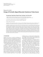
2. RF SYSTEM OVERVIEW
2.1. Transmitter
The block diagram of the transmitter section of our secure
communications system is shown in Figure 1(a).Arandom
noise generator generates a zero-mean band-limited Gaus-
sian noise waveform. This Gaussian noise is passed through
a bandpass filter. The bandpass filter ensures that the signal
is confined within the 1-2-GHz operating frequency range
with a 1.5-GHz center frequency. The output signal n(t)can
be expressed as [17]
n(t)
= a(t)cos

2πf

n
t + θ(t)

,(1)
where a(t) is a Rayleigh distributed random variable, θ(t)isa
uniformly distributed random variable in the range [
−π, π],
and f
n
is the center frequency (1.5-GHz in our case) of
the band-limited noise. This filtered noise is then fed to a
power divider. One output of the power divider connects to
a delay line with a predetermined and controllable delay t
1
.
The delayed signal is amplified and transmitted through a
horizontally polarized antenna working as the reference. The
reference can be mathematically represented as
H(t)
= a

t −t
1

cos

2πf
n

t −t

1

+ θ

t −t
1

. (2)
Without knowledge of this specific delay time, a third party
cannot recover the data even if they know that the message
and reference are being transmitted. Furthermore, assigning
different delay times to different users will allow multiple
users to share the same channel at the same time.
A binary bit sequence m(t) is sent from the digital-to-
analog converter of the field programmable gate array board
to the mixer and is mixed with the 3-GHz (
= f
c
) carrier that is
generated by a phase-locked oscillator. This narrow-band (3-
GHz) modulated radio frequency (RF) message signal is used
as the local oscillator of the single sideband up-converter
and mixed with the filtered band-limited noise from the
other output of the power divider. The single sideband up-
converter can either select the upper sideband (centered at
f
c
+ f
n
) or the lower sideband (centered at f

c
− f
n
)ofthe
mixing process. In our system, the lower sideband is selected.
This noise-like signal is amplified and transmitted through a
vertically polarized antenna which we denote as V(t). The
amplifier gains are adjusted to equalize the transmit power
levels at the two antennas. Clearly, the noise-like signal V(t)
can be expressed as
V(t)
= m(t)a(t)cos

2π

f
c
− f
n

t −θ(t)

. (3)
By judiciously choosing f
c
= 2 f
n
, we ensure that the
lower sideband signal V(t) is located over the same frequency
range as H(t). Thus, the dispersive effects caused by the

atmosphere and other factors are significantly reduced since
both polarization channels operate over the same frequency
band. It is evident that the spread spectrum process is
accomplished within the single sideband up-converter, and
this noise-like signal contains the message that we wish to
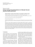
transmit covertly. Since m(t) is either +1 or
−1, the statistical
properties of V(t) should be the same as a zero-mean
band-limited Gaussian random variable. From Figure 2,we
confirm that the spectrum of V(t) is indeed flat over the band
and presents unpredictable behavior in the time domain.
If H(t
k
)andV(t
k
) are the instantaneous magnitudes
of the electromagnetic fields in the horizontal and vertical
polarization channels at time t
k
, respectively, then the instan-
taneous amplitude E(t
k
) and the instantaneous polarization
angle φ(t
k
) (with respect to the vertical) of the composite
transmitted wave are, respectively, given by
E(t
k
) =


H
2

t
k

+ V
2

t
k

,
φ

t
k

= tan
−1

H

t
k

V

t

k


.
(4)
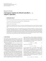
Clearly, the instantaneous amplitude and polarization angle
of the transmitted composite electromagnetic wave are also
random variables. Figure 3 shows the simulation results of
the amplitude and phase plot for the composite electro-
magnetic wave. Since the polarization angle is random, the
Jack Chuang et al. 3
FPGA
m(t)
MXR
SSB
up-converter
AMP
V(t)
V
antenna
OSC
3GHz
Noise
generator
BPF
n(t)
PD
DL
AMP
H(t)

H
antenna
(a)
V
antenna

V(t)
AMP
DL
r(t)
BPF LPF
b(t)
FPGA
H
antenna

H(t)
AMP
OSC
3GHz
(b)
Figure 1: (a) Transmitter block diagram, (b) receiver block diagram. (AMP = amplifier, BPF = bandpass filter, DL = delay line,
FPGA
= fieldprogrammablegatearray,H = horizontal, OSC = oscillator, PD = power divider, SSB = single sideband, V = vertical).
×10
−5
10.80.60.40.20
Seconds
−1
−0.5

0
0.5
1
Amplitude
(a)
×10
9
654321
Frequency
0
100
200
300
400
500
Magnitude
(b)
Figure 2: (a) Time domain and (b) frequency domain plot of
vertically polarized transmitted signal.
composite transmitted signal appears totally unpolarized to
any outside observer. Unlike single carrier communication
systems, the samples of our RF signals have aperiodic
random behavior. It is therefore very difficult for a third party
to recognize that there is a message propagating in the air
since the waveform appears as unpolarized noise, thereby
providing the covertness feature.
2.2. Receiver
The block diagram of the receiver section is shown in
Figure 1(b). For short-range (less than 5km) and low
frequency (less than 20 GHz) applications, we can assume

that the amplitude and phase factors are the same for both
polarization channels, since they are specifically designed so
as to operate over the same frequency band. The received
140120100806040200
Time (ns)
0
0.2
0.4
0.6
0.8
Amplitude
(a)
140120100806040200
Time (ns)
−100
−50
0
50
100
Degree
(b)
Figure 3: (a) Amplitude and (b) polarization angle plot of
composite transmitted electromagnetic wave.
signals

V(t)and

H(t) for the vertically and horizontally
polarized channels, respectively, are given by


V(t) = Am(t)a(t)cos

2π

f
c
− f
n
+ f
d

t −θ(t)

,

H(t) = Aa

t −t
1

cos

2π

f
n
+ f
d

t −t

1

+ θ

t −t
1

,
(5)
where A is the attenuation factor (0
≤ A ≤ 1) causing
by propagation and f
d
is Doppler shift due to moving
transmitter or receiver. In general, A can be considered as
constant when the distance between transmitter and receiver
is small (a few km) under clear atmospheric conditions but
will be a frequency-dependent when the distance becomes
larger or unfavorable atmospheric conditions, such as heavy
rain exists [18].Theperformancewillindeeddegradewhen
the spectrum of received signal is not flat [15]. To overcome
4 EURASIP Journal on Wireless Communications and Networking
this problem, the communication link should ideally esti-
mate attenuation information based on local climatology
and compensate for it at the transmitter, especially when the
system is used for operation over large distances. Without
loss of generality, therefore, we assume that A
= 1. We also
assume perfect carrier synchronization at receiver side, and
therefore f

d
can be considered to be zero without affecting
the following analysis.
The

V(t) signal is amplified and passed through a delay
line with the exact same delay time t
1
as introduced in the
transmitter (for the horizontal channel). It is then mixed
with the

H(t) signal in the mixer, which acts as a correlator.
This brings the two channels in synchronization. If this delay
does not exactly match the corresponding transmit delay,
no message can be extracted from the mixed signal. Only a
friendly receiver knows the exact value of this delay, and thus
an unfriendly receiver will not be able to perform the proper
correlation to decode the hidden message.
The mixed output signal r(t), caused by mixing (i.e.,
multiplying)

V(t − t
1
)and

H(t), containing both the sum
frequency signal s(t) and the difference frequency signal d(t)
can be expressed as
r(t)

= 0.5a
2

t −t
1

m

t −t
1

cos

2πf
c

t −t
1

+0.5a
2

t −t
1

m

t −t
1


cos

2θ

t −t
1

=
s(t)+d(t).
(6)
The difference frequency output containing the random
phase term can be regarded primarily as low-frequency
interference which can be eliminated by filtering. However,
the sum frequency is always centered at f
c
= 2 f
n
and
can be easily demodulated. The bandpass filter centered
at f
c
following the first mixer in the receiver will capture
the desired sum frequency signal while discarding the low-
frequency interference. The filtered RF signal is mixed with
the output of an oscillator at f
c
(3 GHz in our system) in
ordertostripoff the carrier. The received baseband signal
b(t) at the output of the low-pass filter is expressed as
b(t)

= 0.25a
2

t −t
1

m

t −t
1

⊗
h(t), (7)
where h(t) is filter impulse response. Since binary modula-
tion is used and the a
2
(t − t
1
) term is always positive, the
transmitted bit sequence can be successfully retrieved from
b(t).
3. SYSTEM PERFORMANCE MODELING
In wireless communications, the bit error rate (BER) is
an important metric which is used to gauge and compare
the system performance. Since this noise modulated covert
communications system is a new architecture, the theoretical
BER performance in an additive white Gaussian noise
channel is derived and compared with simulation results in
this section. Unlike other single-channel spread spectrum
systems, the low-pass equivalent model can directly be used

to model the system behavior in the Gaussian channel.
The spreading and dispreading process of our system is
accomplished at the RF front-end. The noise floor at the
antenna output is not the same as that at the output of
the first mixer, and the noise terms within the system are
generated by mixing of two zero mean independent Gaussian
random variables. Thus, the system behavior needs to be
modeled based upon the relationship between the SNR at the
output of receiver antenna and the probability of bit error. In
this section, we will demonstrate that the mixed noise can be
approximated as Gaussian after passing through a narrow-
band filter, and the BER equation can be expressed using the
Q-function. The bandwidths of the signal, antenna, low-pass
filter, and the SNR at the output of receiver’s antenna are
the parameters which dominate the BER when the bit rate
is fixed.
To simplify the analysis, we assume that the delay term
t
1
is set to zero in both the transmitter and the receiver. This
simplification will not affect the BER analysis. In an additive
white Gaussian noise channel, the actual received signal from
the vertically polarized antenna

V(t) and the horizontally
polarized antenna

H(t) can be written, respectively, as

V(t) =


V(t)+n
V
(t),

H(t) =

H(t)|
t
1
=0
+ n
H
(t).
(8)
The n
V
(t)andn
H
(t) terms are independent zero-mean
band-limited Gaussian noise in the vertical and horizontal
polarization channels, and these terms are also independent
of

V(t)and

H(t). Their analytical forms are similar to n(t)as
shown in (1), that is,
n
V

(t) = a
V
(t)cos

2πf
n
+ θ
V
(t)

,
n
H
(t) = a
H
(t)cos

2πf
n
+ θ
H
(t)

,
(9)
where a
V,H
and θ
V,H
are the polarization dependent random

Rayleigh-distributed amplitude and uniformly-distributed
phaseterms,respectively.Thepowerofn
V
(t)andn
H
(t)is
equal to their variance since they are zero-mean random
variables and these are denoted as σ
2
V
and σ
2
H
,respectively.
We further assume that the powers of

V(t)and

H(t), both
of which are zero-mean band-limited Gaussian processes,
are the same, and each is denoted as σ
2
S
. The corresponding
SNR values at the output of vertical and horizontal polarized
antennas are σ
2
S
/σ
2

V
and σ
2
S
/σ
2
H
,respectively,andaredenoted
as SNR
V
and SNR
H
. In reality, the bandwidth of V(t)is
slightly greater than that of H(t) due to the modulation m(t)
induced on it. However, the bandwidth of m(t)isverysmall
compared with H(t). We assume that the signal bandwidth
of V(t)andH(t) (hence the bandwidth of

V(t)and

H(t)) is
B
S
, and that the bandwidth of n
V
(t)andn
H
(t)isB
n
(equal

to the receive antenna bandwidth). Usually, B
S
is almost the
same as B
n
in order to avoid receiving additional interference.
Down the receiver chain, the noisy signals

V(t − t
1
) =

V(t)and

H(t) are mixed together, and the mixed signal S(t)
contains the desired signal term

V(t)

H(t) (first term below)
and three interference cross-terms given by
S(t)
=

V(t)

H(t)+n
V
(t)


H(t)+n
H
(t)

V(t)+n
V
(t)n
H
(t).
(10)
Jack Chuang et al. 5
In the real system implementation, the bandpass filter is
used to capture just the sum frequency signal centered
at f
c
(3 GHz) containing the information message, while
discarding all difference frequency signals contained in S(t)
is discarded as noise. Let BPF(x(t)) denote the bandpass
filtered output of the signal x(t). The bandpass filtered
noise signals are denoted as n
1
(t), n
2
(t), and n
3
(t), where
n
1
(t) = BPF(n
V

(t)

H(t)), n
2
(t) = BPF(n
H
(t)

V(t)), and
n
3
(t) = BPF(n
H
(t)n
V
(t)). Generally, the probability density
function of the noise needs to be found in order to calculate
the BER. Since the probability density function of the
product of two independent zero-mean normal distributions
is approximated by a modified Bessel function of the second
kind, the closed form probability density function for the
sum n
1
(t)+n
2
(t)+n
3
(t) is extremely difficult to derive.
Because the bandwidth of filtered noise is much smaller than
before filtering, the noise spectrum following the filter is

relatively flat compared to the sum frequency noise. Thus,
we can approximate the filtered noise as a Gaussian variable.
For convenience, we assume that the bandwidth of the
bandpass filter is twice that of the low-pass filter following
the second down-conversion, since the low-pass filter is the
key component dominating the received noise spectrum
before the decision circuit. Later in this section, we will
compare the theoretical results with simulation results to
show that our derivation by applying this assumption also
works when the bandwidth of bandpass filter is much greater
than bandwidth of low-pass filter.
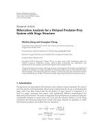
Based on our simulation analysis, a cumulative distri-
bution function comparison between n
1
(t)(arepresentative
interference term) and a zero-mean band-limited Gaussian
with the same power and frequency range is shown in
Figure 4. In the simulation, the bandwidth of bandpass filter
is 40 MHz (B
L
= 20 MHz), the bandwidth of signal B
S
is 970 MHz, and the bandwidth of the channel noise B
n
is 980 MHz. We note that the two cumulative distribution
function plots are very close. Thus, these results validate our
assumption that the filtered sum frequency noise terms can
be approximated as Gaussian.
After realizing that the filtered noise terms can be
approximated as Gaussians, their means and variances need

to be found for calculating the BER. The mean value of n
1
(t)
is found as zero, as seen from
E

n
1
(t)

=
E


∞
−∞
h(τ)n
V
(t −τ)H(t − τ)dτ

=

∞
−∞
h(τ)E

n
V
(t −τ)


E

H(t − τ)

dτ
= 0,
(11)
where h(τ) is impulse response of bandpass filter [19].
Similarly, the mean values of n
2
(t)andn
3
(t) are both zero.
The next step is to calculate the variance of the filtered
noise, which is equal to its power. Clearly, the power of
n
1
(t), n
2
(t), and n
3
(t) can be calculated by integrating the
power spectrum of the sum frequency noise of n
V
(t)

H(t),
n
H
(t)


V(t), and n
V
(t)n
H
(t) within the bandpass filter fre-
quency range.
10.80.60.40.20
CDF comparison
n
1
(t)
Zero-mean Gaussian
0
0.1
0.2
0.3
0.4
0.5
0.6
0.7
0.8
0.9
1
CDF
Figure 4: Cumulative distribution function comparison between
zero-mean Gaussian and bandpass filtered noise term.
Let the power spectral density of the sum frequency
noise of n
V

(t)

H(t)bedenotedasS
n
V

H
( f ). The average
power of the sum frequency noise needs to be found first
in order to find the mathematical expression for S
n
V

H
( f ).
We know that for a given ergodic random process x(t),
its autocorrelation function R
xx
(τ) and its power spectral
density S
x
( f ) form a Fourier transform pair, that is, R
xx
(τ) ↔
S
x
( f ). Furthermore, the average power of such a random
process is the value of the autocorrelation function at zero
lag, that is, equal to R
xx

(0).
The sum frequency noise of n
V
(t)

H(t), noting that t
1
=
0, can be expressed as
N
1
(t) = 0.5a(t)a
V
(t)cos

2πf
c
+ θ
V
(t)+θ(t)

. (12)
The average power of N
1
(t) can be determined from its
autocorrelation function with the lag τ set equal to zero and
can be expressed as
P
S
= E


(0.5a(t)a
V
(t)cos(2πf
c
t + θ(t)+θ
V
(t)))
2

=
0.125E

a
2
(t)a
2
V
(t)cos

4πf
c
t +2θ(t)+2θ
V
(t

)

+0.125E


a
2
(t)a
2
V
(t)

=
0.125E

a
2
(t)

E

a
2
V
(t)

.
(13)
Recognizing that a(t)anda
V
(t) are independent Rayleigh
distributed random variables. Furthermore, the kth moment
of a Rayleigh distributed random variable x is noted as [19]
E


x
k

=
⎧
⎪
⎨
⎪
⎩
1·3 ···kσ
k

π
2
,
k
= 2n +1,
2
n
n!σ
2n
,
k
= 2n,
(14)
6 EURASIP Journal on Wireless Communications and Networking
where
√
πσ
2

/2 is the mean. For k = 2, that is, n = 1, we have
E[a
2
(t)] = 2σ
2
S
and E[a
2
V
(t)] = 2σ
2
V
. We therefore have
P
S
= 0.5σ
2
S
σ
2
V
. (15)
Thus, the value of the corresponding power spectral
density of the sum frequency noise S
n
V

H
( f ) integrated
over frequency is 0.5σ

2
S
σ
2
V
. Since the sum frequency noise
n
V
(t)

H(t) is the product of two band-limited rectangular
spectra centered at f
n
= f
c
/2 with bandwidths B
n
and B
S
(B
S
≈ B
n
), respectively, S
n
V
,

H
( f ) has an isosceles triangle

shape centered also at f
c
with an overall bandwidth equal to
B
n
+ B
S
. Therefore, S
n
V
,

H
( f ) can be expressed as
S
n
V
,

H
( f )
=
⎧
⎪
⎪
⎪
⎪
⎪
⎨
⎪

⎪
⎪
⎪
⎪
⎩
−
2σ
2
V
σ
2
S


f − f
c



B
n
+ B
S

2
+
σ
2
V
σ

2
S
B
n
+ B
S
, f
c
−0.5

B
n
+ B
S

≤ f
≤ f
c
+0.5

B
n
+ B
S

,
0, otherwise.
(16)
The power of n
1

(t) contained within the low-pass filter
bandwidth B
L
can be finally found from
P
n1
=

f
c
+B
L
f
c
−B
L
S
n
V
,

H
( f )df = 0.5G
1
σ
2
S
σ
2
V

, (17)
where G
1
is given by
G
1
=

1 −

1 −
2B
L
B
n
+ B
S

2

. (18)
In a similar manner, n
2
(t)andn
3
(t)canbederivedas
0.5G
1
σ
2

S
σ
2
H
and 0.5G
2
σ
2
V
σ
2
H
,respectively,whereG
2
is given by
G
2
=

1 −

1 −
B
L
B
n

2

. (19)

The summation of n
1
(t), n
2
(t), and n
3
(t), representing the
total interference component, is also a zero-mean band-
limited Gaussian random variable and we denote it as n(t).
The variance of n(t) is equal to its average power and is given
by
var(n)
= var

n
1

+var

n
2

+var

n
3

+cov

n

1
, n
2

+cov

n
1
, n
3

+cov

n
2
, n
3

.
(20)
Since n
1
(t), n
2
(t), and n
3
(t) are uncorrelated zero-mean
Gaussian distributions, the covariance terms are zero, and
therefore, the interference power is obtained as
var(n)

= 0.5

G
1
σ
2
S
σ
2
V
+ G
1
σ
2
S
σ
2
H
+ G
2
σ
2
V
σ
2
H

. (21)
The n(t) term is mixed with the 3-GHz carrier and down
to the baseband with a power that is equal to 0.125(G

1
σ
2
S
σ
2
V
+
G
1
σ
2
S
σ
2
H
+ G
2
σ
2
V
σ
2
H
). Since the baseband noise is zero-mean
Gaussian and binary modulation is used, the BER equation
for the optimal receiver can be expressed by the Q-function
with two parameters: the spectrum magnitude of the noise
(N
0

) and the bit energy (E
b
)[20, 21].
From (7), when there is no low-pass filter truncating
the signal spectrum, the average power of received baseband
signal can be found using the fourth moment of a(t) and is
shown to be
P
b
≈ E

0.25a
2
(t)

2

=
0.5σ
4
S
. (22)
Since the a
2
(t)termin(7) will spread out the baseband
signal power over a frequency range wider than the low-
pass filter bandwidth, the low-pass filter at the receiver will
truncate the signal spectrum, and the received power will
be lower than the value obtained in (22). Therefore, the bit
energy at the output of low-pass filter can be expressed as

0.5ρσ
4
S
T
b
when bit duration time is T
b
.Theρ is the power
loss factor due to the filtering, defined as the ratio between
the truncated baseband signal power after the low-pass filter
to the untruncated baseband signal. Clearly, the loss factor
satisfies 0
≤ ρ ≤ 1. From above discussion, the BER of the
noise modulated covert communication system with a two-
sided spectrum can be mathematically expressed as
P
e
= Q


2E
b
N
0

=
Q
⎛
⎝





8ρσ
4
S
T
b
B
L
G
1
σ
2
S
σ
2
V
+ G
1
σ
2
S
σ
2
H
+ G
2
σ
2

V
σ
2
H
⎞
⎠
.
(23)
The well-known Q(x) function is shown below for reference
as
Q(x)
=
1
√
2π

∞
x
e
−y
2
/2
dy. (24)
Equation (23) can be also expressed using SNR
V
and SNR
H
as follows:
P
e

= Q


8ρT
b
B
L
G
1
SNR
−1
V
+ G
1
SNR
−1
H
+ G
2
SNR
−1
V
SNR
−1
H

.
(25)
A full system simulation in an additive white Gaussian
noise channel was done to validate the theoretical results in

(25), and the results are shown in Figures 5 and 6. In the
simulation, both the SNR
V
and the SNR
H
terms are equal,
and the bandwidth of the antenna is 10 MHz wider than
the bandwidth of the transmitted signal in order to avoid
truncation of the wider spectrum caused by the modulation.
The bandpass filter has a bandwidth of 100 MHz and is
centered at 3 GHz. In Figure 5, a low-pass filter bandwidth of
10 MHz is used for the simulation. The value of ρ depends
on the bit rate and the low-pass filter bandwidth. From
our independent simulation result, for a bit rate of 5 Mbps,
the value of ρ was determined to be approximately 0.487
when the transmitted signal bandwidth is 970 MHz and
approximately 0.5 when the transmitted signal bandwidth
is 500 MHz. In Figure 6, the low-pass filter bandwidth is
20 MHz, and the signal bandwidth is 970 MHz bandwidth in
the simulation. The value of ρ was determined to be 0.49,
0.5, and 0.518 when the bit rate is 10 Mbps, 5 Mbps, and
2 Mbps, respectively. From Figures 5 and 6, we note that
Jack Chuang et al. 7
the maximum deviation between the simulation results and
theoretical results is 0.5 dB. Thus, the system behavior of this
ultrawideband communication system is properly modeled.
As the bandwidth of V(t)andH(t) is increased, the noise
power will be dispersed into larger frequency ranges after the
mixing process, and the system performance will improve
because the processing gain will increase.

4. MULTIUSER MODELING
In a multiuser environment, each user uses the same channel
but is assigned a different delay. The receiver contains
a switchable delay bank between the vertical polarization
antenna and the first mixer to select a particular user. If σ
2
i
is the signal power of

V
i
(t)and

H
i
(t) corresponding to the
ith user, the received signals in the vertically and horizontally
polarized antennas in an additive white Gaussian noise
channel are given by

V
N
(t) =
N

i=1

V
i
(t)+n

V
(t), (26)

H
N
(t) =
N

i=1

H
i

t −t
i

+ n
H
(t), (27)
when there are N users in the channel. The t
i
term in (27)
is the specific delay time assigned to the ith user, and the
receiver already knows this information. Since the output
signals of different noise generators are independent of each
other, the

V
i
(t) terms are independent to each other and so

are the

H
i
(t)terms.
For any user who wants to receive the message from the
ith user, the delay line with the delay t
i
between vertical
polarization antenna and the first mixer in the receiver is
activated. Then, the signal at the output of the first mixer can
be written as
S
N
(t) =

V
i

t −t
i


H
i

t −t
i

+

N

n=1
N

m=1

V
m

t −t
i


H
n

t −t
n

+
N

m=1


V
m

t −t

i

n
H
(t)+

H
m

t −t
m

n
V

t −t
i

+ n
V

t −t
i

n
H
(t), (m, n)
/
=(i, i).
(28)

Thesecondtermin(28) can be considered as interference
and its characteristics are similar to the third and fourth
terms when the difference between each t
i
term is large
enough. Thus, the sum frequency signal in (28) contains
N
2
− 1 interference terms with bandwidth 2B
S
,2N interfer-
ence terms with bandwidth B
S
+ B
n
, and one interference
term with bandwidth 2B
n
. All the interference terms are
centered at f
c
. Using the same method that was used to derive
the BER for the single-user environment, the BER equation
for N users in the additive white Gaussian noise channel can
be mathematically expressed as
P
e
= Q
⎛
⎝


8ρσ
4
i
T
b
B
L
H
⎞
⎠
,(m, n)
/
=(i, i), (29)
−6−7−8−9−10−11
SNR at antenna output (dB)
BW
= 970 MHz (simulation)
BW
= 970 MHz (theory)
BW
= 500 MHz (simulation)
BW
= 500 MHz (theory)
10
−5
10
−4
10
−3

10
−2
10
−1
10
0
Probability of error
Bandwidth vs. BER
Figure 5: Comparison of SNR and BER characteristics between
simulation and theory in a single user environment at different
signal bandwidths.
where
H
= G
3
N

n=1
N

m=1
σ
2
n
σ
2
m
+ G
1
N


m=1

σ
2
m
σ
2
H
+ σ
2
m
σ
2
V

+ G
2
σ
2
V
σ
2
H
.
(30)
The G
1
and G
2

terms are shown in (18)and(19), respectively,
and G
3
is given by
G
3
=

1 −

1 −
B
L
B
S

2

. (31)
In our simulation, we assume that each user has the same
power, in which case, (29)reducesto
P
e
= Q


Z

, (32)
where

Z
=
8ρσ
4
S
T
b
B
L

N
2
−1

G
3
σ
4
S
+ G
1
N

σ
2
S
σ
2
H
+ σ

2
S
σ
2
V

+ G
2
σ
2
V
σ
2
H

.
(33)
The bit rate is 5 Mbps, and the bandwidth of antenna and the
signal is 980 MHz and 970 MHz, respectively. The simulation
results are shown in Figure 7 from which we note that the
deviation between the simulation results and theoretical
results is less than 0.5 dB. As the number of users increases,
the noise floor also increases and the BER degrades.
5. COMPREHENSIVE EXPERIMENTAL RESULTS
As a test of the noise modulated covert communication
system functionality, comprehensive tests were performed.
8 EURASIP Journal on Wireless Communications and Networking
−9−10−11−12−13−14
SNR at antenna output (dB)
10 Mbits/s (simulation)

10 Mbits/s (theory)
5 Mbits/s (simulation)
5 Mbits/s (theory)
2 Mbits/s (simulation)
2 Mbits/s (theory)
10
−4
10
−3
10
−2
10
−1
10
0
Probability of error
Antenna BW = 980MHz
Figure 6: Comparison of SNR and BER characteristics between
simulation and theory in a single user environment at different bit
rates.
−4−5−6−7−8−9−10−11
SNR at antenna output (dB)
3 users (simulation)
3 users (theory)
5 users (simulation)
5 users (theory)
10
−4
10
−3

10
−2
10
−1
10
0
Probability of error
Multiuser
Figure 7: Comparison of SNR and BER characteristics between
theory and simulation in a multiuser environment.
A Lyrtech field programmable gate array board samples the
audio wave and translates it into binary bit stream. This
bit stream is interpreted as +/– voltage by the digital to
analog converter and is mixed with a 3-GHz carrier as radio
frequency modulated signal. At the transmitter, a 1-2-GHz
noise source is used. The noise source is connected to a
1.2–1.8-GHz bandpass filter and then to a power divider.
The RF modulated signal and filtered noise are sent to a
single sideband up-converter, and then the lower sideband is
chosen as the transmitted signal in the vertical channel. The
antennas used at the transmitter and receiver are dual linear
horn antennas. At the receiver side, the 40-dB gain limiting-
amplifiers are connected after the antennas in order to drive
the mixer in the square-low region. A 2.9–3.1-GHz bandpass
filter and two 14-dB gain amplifiers are connected after the
mixer at the receiver. The output of the amplifier is connected
to the second mixer, and then to a 1.9-MHz bandwidth
low-pass filter. The low-pass filter is connected to another
Lyrtech board, and the audio is recovered. In the experiment,
the system is placed in the open field with grass terrain

and the distance between the transmitter and receiver is 30
meters. An additional 10-dB attenuator is added to imitate
a distance of 94 meters. Since the carrier synchronization
loop is not built in the receiver, an Agilent E4438C vector
signal generator is used as a common frequency source. The
experimental setup and system implementation are shown in
Figure 8.
All the baseband signal processing is implemented on
Lyrtech SignalWAVe DSP/FPGA development boards. Using
Xilinx ISE 7.0 and the Xilinx and Lyrtech blocksets, the
baseband signal processing was designed in the Simulink
environment and then loaded into the Lyrtech board. The
transmitter design is shown in Figure 9(a). An audio signal
is sampled by the audio codec with sample frequency
approximately equal to 3.85 kHz and then quantized into
a 14-bit frame. The 14-bit header [1,0,1,1,1,0,1,0,1,0,0,0,0]
is inserted between every 7000 data frames and then the
bit stream with the header is sent to the digital-to-analog
converter where bit-1 and bit-0 are represented as +/–
voltages. The receiver baseband signal processing design is
shown in Figure 9(b). At the output of the low-pass filter,
hard decisions are made by taking the sign (output 1 or
−1)
of the incoming samples. The resulting sequence is passed
through the framing and timing synchronization circuits to
ensure that the serial to parallel block is activated at the
proper times and then the received data frame is transformed
back into the original sample values and the audio can be
recovered.
At the receiver side, the received signals at the output

of vertical polarization antenna and horizontal polarization
antenna are at power levels of
−56 dBm and −57 dBm,
respectively. The Agilent DSO-80804B oscilloscope is used
to record the received V(t), a plot of which is shown in
Figure 10. Our signal does show random behavior in the
time domain and flat spectrum in the frequency domain.
The spectrum is not perfectly flat because the conversion loss
of the single sideband up-converter is not entirely constant
over the 1.2–1.8-GHz band. The peaks around 900 MHz
and 1900 MHz are caused by the cell phone signals, and the
one around 1900 MHz is considered as interference because
it will generate extra interference terms after the mixing
process.
In the field test, the audio could be heard with good
quality. Due to the unknown and uncertain delay caused by
wiring and the propagation channel, it is difficult to directly
compare the input and the output audio waveforms. By
properly modifying the baseband signal processing design,
the system will send a header continuously with a bit rate of
Jack Chuang et al. 9
(a) (b)
BPF
Noise
generator
AMP
PD
AMP
SSB
up-converter

MXR
(c)
BPF
MXR
AMP
MXR
LPF
(d)
Figure 8: (a) Transmitter view, (b) receiver view, (c) transmitter and (d) receiver layout.
approximately 110 Kbps. Thus, we can compare the sent and
received bit streams in an ideal channel and a noisy channel.
Figure 11 shows the transmitted bit stream (a) and the
received bit stream (b) in the ideal channel. The waveform
is recorded by the Agilent DSO-80804B oscilloscope at the
output of the low-pass filter. We note that the ideal channel
amplitude fluctuations, caused by the random a
2
(t)term,
will not affect the decision for binary modulation. Figure 11
also shows the same bit stream being received in an additive
white Gaussian noise channel (c) and a channel containing
tone interference (d).
The zero crossings show up when the channel is not clean
but the message can still be retrieved. Although not shown,
when both tone interferences are located within the narrow
frequency range (0.5 f
c
− B
L
<f<0.5 f

c
+ B
L
) in the low-
SIR channel, the bit stream is ruined because of high-power
tone interference at the output of low-pass filter generated
by the sum frequency signal of the tone interference in the
V-channel mixed with the tone interference in H-channel.
Usually, this problem can be solved by adding a digital filter
in the baseband signal processing design.
In practice, polarization mismatch may occur between
transmitter and receiver antennas and this is an important
factor that will affect system performance. When the anten-
nas at either end are not perfectly aligned, there will exist
a rotation angle between the antenna axes at either end.
Thus, each polarization channel at the receiver side not only
receives the desired received signal but also the leakage from
the orthogonal polarization component. The signals that
send from V-channel and H-channel to the first mixer at the
receiver side can then be expressed as

V(t) = α

V

t −t
1

+ β


H

t −2t
1

+ n
V

t −t
1

,

H(t) = α

H

t −t
1

+ β

V(t)+n
H
(t),
(34)
where t
1
is the delay time of the delay line (t
1

 B
−1
S
in the
system implementation), β

H(t − 2t
1
) is the received leakage
from the transmit H-channel into the receive V-channel, and
β

V(t) is the received leakage from the transmit V-channel
into the received H-channel. The terms α and β are the
square root of polarization loss factor with value depending
on the rotation angle. They are within the range [0, 1] and
α
2
+ β
2
= 1[22]. For perfect antenna alignment, α = 1and
β
= 0, and there is no polarization leakage.
As the rotation angle increases, the value of β increases
while the value of α decreases. When the rotation angle is 45
degrees, α
= β =
√
0.5. The worst case occurs at a rotation
angleof90degreesbecausethepowerofdesiredreceived

signal is zero and no message can be extracted from the
10 EURASIP Journal on Wireless Communications and Networking
Adding header
Out
Counter
a
b
a>b
Relational
>
Cast
Convert5
Sel
d0
d1
PCM3008
acquisition
DSP bus
Tx
k
= 14
Constant
Out1
Header
Cast
Convert2
×1.638e+
004
CMult2
Cast

Convert4
DAC1
DAC1
Output
To
workspace
To
mixer
Bus0
DSP bus
Codec Sync
Cast
Convert
PS
Parallel to serial
(a)
Framing and timing
synchronization
ADC1
ADC1
sgn
From the output of LPF
Threshold
X>>1
Shift
Counter1
Out
z
−1
Delay

In1
Out1
Out2
HeaderDetector2
d
en
z
−1
q
Register4
reg
fd
Out1
Delay offset
shift register
Cast
Convert1
DSP bus
Rx
Codec Sync
Bus0
DSP bus1
Time
Output
PCM3008
playback
(b)
Figure 9: (a) Transmitter baseband signal processing design, (b) receiver baseband signal processing design.
received signal (α = 0, β = 1). The BER equation upon
considering nonperfect alignment in a Gaussian channel can

be expressed as
P
e
= Q
⎛
⎝




8ρα
4
σ
4
S
T
b
B
L
G
3

2α
2
β
2
+ β
4

σ

4
S
+ Y + G
2
σ
2
V
σ
2
H
⎞
⎠
, (35)
where
Y
= G
1

α
2
+ β
2

σ
2
S
σ
2
H
+ σ

2
S
σ
2
V

, (36)
and G
1
, G
2
, G
3
are as shown in (18), (19), and (31). Com-
paring (35)with(23), nonperfect antenna alignment will
degrade system performance because it generates extra inter-
ference terms and decreases the power of desired received
signal. A method for measuring the rotation angle is to send
a pilot tone from one of the dual-polarization channels and
use the power ratio between received V-channel signal and
received H-channel signal to determine the rotation angle.
To simplify the structure, better estimation technique should
be developed for measuring rotation angle without using a
pilot.
6. CONCLUSIONS
A spread spectrum technique using noise-modulated wave-
forms is proposed for covert communications. The fea-
tureless characteristics of the transmitted waveform in the
noise modulated covert communication system ensure the
security of communications. By using a band-limited true

Gaussian noise waveform to spread the signal’s power into
a large bandwidth, an extremely large processing gain is
achieved and the system can operate very well in a low
SNR or SIR channel. Based on our current research, the
“cross-multiplication” method could alleviate performance
degradation caused by multipath. The underlying concept
Jack Chuang et al. 11
×10
−7
987654321
Time (s)
−4
−2
0
2
4
×10
−3
Magnitude (V)
(a)
×10
9
2.221.81.61.41.210.8
Frequency (Hz)
−180
−170
−160
−150
−140
−130

Power spectral density (dB/Hz)
(b)
Figure 10: (a) Recorded time domain of received V(t), (b) recorded
frequency domain of received V(t).
×10
−4
1.81.61.41.210.80.60.40.20
Time (s)
−0.4
0
0.4
Magnitude (V)
(a)
×10
−4
1.81.61.41.210.80.60.40.20
Time (s)
−0.1
0
0.1
Magnitude (V)
(b)
×10
−4
1.81.61.41.210.80.60.40.20
Time (s)
−0.05
0
0.05
Magnitude (V)

(c)
×10
−4
1.81.61.41.210.80.60.40.20
Time (s)
−0.05
0
0.05
Magnitude (V)
(d)
Figure 11: (a) Original transmitted bit stream, (b) bit stream
received in ideal channel, (c) bit stream received in additive white
Gaussian noise channel, (d) bit stream received in single-tone
interference channel.
of this method is to synchronize the nth path in the
V-channel with the mth path in the H-channel instead
of directly synchronizing the received V-channel and H-
channel signals. Without considering system complexity,
combining a pseudonoise sequence with our method can
show better performance than a RAKE receiver since more
diversity can be used. For example, if each channel contains
N multipath terms, there are N diversity that can be used
by the RAKE receiver but N
2
diversity can be used by our
method.
The performance of this noise modulated covert com-
munication system in a single and multiuser environment
is properly modeled and compared with simulations. The
bandwidth of the transmitted signal and antenna controls the

BER performance when the SNR at the output of antenna
and bit rate is fixed. The field tests demonstrate that the
concept can be realized, and the system can operate in an
additive white Gaussian noise channel with negative SNR.
ACKNOWLEDGMENTS
This work is supported by the Office of Naval Research
(ONR) under Contract no. N00014-04-1-0640. The authors
appreciate fruitful discussions with Mr. John Moniz and Mr.
Timothy Wasilition of ONR. They thank Dr. Sven Bilen of
The Pennsylvania State University for supplying the two-
field programmable gate array boards for the experiments.
Moreover, they also thank Star-H Corporation, Pa, USA , for
providing the location for the field tests and Arhan Gunel,
Keith Newlander, and Paul Bucci for their help in the field
testing.
REFERENCES
[1] C. E. Cook and H. S. Marsh, “An introduction to spread
spectrum,” IEEE Communications Magazine,vol.21,no.2,pp.
8–16, 1983.
[2] R. A. Scholtz, “The origins of spread-spectrum communica-
tions,” IEEE Transactions on Communications,vol.30,no.5,
part 2, pp. 822–854, 1982.
[3] P. C. J. Hill, V. E. Comley, and E. R. Adams, “Techniques for
detecting and characterizing covert communication signals,”
in Proceedings of the IEEE Military Communications Conference
(MILCOM ’97), vol. 3, pp. 1361–1365, Monterey, Calif, USA,
November 1997.
[4] M. Gouda, E. R. Adams, and P. C. J. Hill, “Detection & dis-
crimination of covert DS/SS signals using triple correlation,”
in Proceedings of the 15th National Radio Science Conference

(NRSC ’98), pp. C35/1–C35/6, Cairo, Egypt, February 1998.
[5] G. Burel, “Detection of spread spectrum transmissions using
fluctuations of correlation estimators,” in Proceedings of the
IEEE International Symposium on Intelligent Signal Processing
and Communication Systems (ISPACS ’00), pp. 1–6, Honolulu,
Hawaii, USA, November 2000.
[6] N.C.Beaulieu,W.L.Hopkins,andP.J.McLane,“Interception
of frequency-hopped spread-spectrum signals,” IEEE Journal
on Selected Areas in Communications, vol. 8, no. 5, pp. 853–
870, 1990.
12 EURASIP Journal on Wireless Communications and Networking
[7] G. R. Cooper and L. H. Cooper, “Covert communication with
a purely random spreading function,” in Proceedings of the
IEEE Military Communications Conference (MILCOM ’82),pp.
2.4-1–2.4-2, Boston, Mass, USA, October 1982.
[8] L. Turner, “The evolution of featureless waveforms for
LPI communications,” in Proceedings of the IEEE National
Aerospace and Electronic s Conference (NAECON ’91), vol. 3,
pp. 1325–1331, Dayton, Ohio, USA, May 1991.
[9] K. M. Cuomo, A. V. Oppenheim, and S. H. Strogatz, “Synchro-
nization of Lorenz-based chaotic circuits with applications to
communications,” IEEE Transactions on Circuits and Systems
II, vol. 40, no. 10, pp. 626–633, 1993.
[10] C. K. Rushforth, “Transmitted-reference techniques for ran-
dom or unknown channels,” IEEE Transactions on Information
Theory, vol. 10, no. 1, pp. 39–42, 1964.
[11] R. M. Gagliardi, “A geometrical study of transmitted reference
communication systems,” IEEE Transactions on Communica-
tion Technology, vol. 12, no. 4, pp. 118–123, 1964.
[12] M H. Chung and R. A. Scholtz, “Comparison of transmitted-

and stored-reference systems for ultrawideband communica-
tions,” in Proceedings of the IEEE Military Communications
Conference (MILCOM ’04), vol. 1, pp. 521–527, Monterey,
Calif, USA, October-November 2004.
[13] T. Q. S. Quek and M. Z. Win, “Analysis of UWB transmitted-
reference communication systems in dense multipath chan-
nels,” IEEE Journal on Selected Areas in Communications, vol.
23, no. 9, pp. 1863–1874, 2005.
[14] T. Q. S. Quek, M. Z. Win, and D. Dardari, “Unified anal-
ysis of UWB transmitted-reference schemes in the presence
of narrowband interference,” IEEE Transactions on Wireless
Communications, vol. 6, no. 6, pp. 2126–2139, 2007.
[15] R. M. Narayanan and J. Chuang, “Covert communications
using heterodyne correlation random noise signals,” Elect ron-
ics Letters, vol. 43, no. 22, pp. 1211–1212, 2007.
[16] J. Chuang, M. W. DeMay, and R. M. Narayanan, “Secure
spread spectrum communication using ultrawideband ran-
dom noise signals,” in Proceedings of the IEEE Military Com-
munications Conference (MILCOM ’07), pp. 1–7, Washington,
DC, USA, October 2007.
[17] M. Dawood and R. M. Narayanan, “Receiver operating
characteristics for the coherent UWB random noise radar,”
IEEE Transactions on Aerospace and Electronic Systems, vol. 37,
no. 2, pp. 586–594, 2001.
[18] K. M. Mohan, Covert communication system u sing random
noise signals: propagation and multipath effects, M.S. thesis,
The Pennsylvania State University, University Park, Pa, USA,
December 2005.
[19] A. Papoulis and S. U. Pillai, Probability, Random Variables, and
Stochastic Processes, McGraw-Hill, New York, NY, USA, 4th

edition, 2002.
[20]R.L.Peterson,R.E.Ziemer,andD.E.Borth,Introduction
to Spread Spectrum Communications, Prentice-Hall, Upper
Saddle River, NJ, USA, 1995.
[21] G. K. Kaleh, “Frequency-diversity spread spectrum communi-
cation system to counter bandlimited Gaussian interference,”
IEEE Transactions on Communications, vol. 44, no. 7, pp. 886–
893, 1996.
[22] C. A. Balanis, Antenna Theory: Analysis and Design,JohnWiley
& Sons, New York, NY, USA, 3rd edition, 2005.